State of Health Estimation of Lithium-Ion Batteries in Electric Vehicles under Dynamic Load Conditions

Abstract

Among numerous functions performed by the battery management system (BMS), online estimation of the state of health (SOH) is an essential and challenging task to be accomplished periodically. In electric vehicle (EV) applications, accurate SOH estimation minimizes failure risk and improves reliability by predicting battery health conditions. The challenge of accurate estimation of SOH is based on the uncertain dynamic operating condition of the EVs and the complex nonlinear electrochemical characteristics exhibited by the lithium-ion battery. This paper presents an artificial neural network (ANN) classifier experimentally validated for the SOH estimation of lithium-ion batteries. The ANN-based classifier model is trained experimentally at room temperature under dynamic variable load conditions. Based on SOH characterization, the training is done using features such as the relative values of voltage, state of charge (SOC), state of energy (SOE) across a buffer, and the instantaneous states of SOC and SOE. At implementation, due to the slow dynamics of SOH, the algorithm is triggered on a large-scale periodicity to extract these features into buffers. The features are then applied as input to the trained model for SOH estimation. The classifier is validated experimentally under dynamic varying load, constant load, and step load conditions. The model accuracies for validation data are 96.2%, 96.6%, and 93.8% for the respective load conditions. It is further demonstrated that the model can be applied on multiple cell types of similar specifications with an accuracy of about 96.7%. The performance of the model analyzed with the confusion matrices is consistent with the requirements of the automotive industry. The classifier was tested on a Texas F28379D microcontroller unit (MCU) board. The result shows that an average real-time execution speed of 8.34 µs is possible with a negligible memory occupation.

1. Introduction

Lithium batteries are finding application as the major energy source and storage device in many electrical and electronic devices, especially in electric, plugin electric, and hybrid vehicles. Energy management in electric vehicle powertrain requires accurate measurement of the battery state of charge (SOC) to ensure safety. Accurate SOC measurement enhances energy balancing and reliability in energy distribution [1,2]. To ensure accurate SOC estimation, it is necessary to continuously update the SOC estimation algorithm in the battery management system (BMS) with the health status of the battery. The performance of lithium-ion batteries is affected by both calendar aging and cycling [3]. Some commonly used indices for measuring battery aging in the literature are the remaining useful (RUL) and the state of health (SOH) [4,5]. The computation of the SOH and RUL accounts for the capacity fading and hence the aging of the battery.

SOH has been investigated through various experimental, model-based, and machine learning methods in the literature. Experimental methods try to measure SOH directly, and they are suitable for stationary and laboratory applications. The specific equipment required and the complex procedures however make it costly and time-demanding. The experimental methods for SOH estimation comprise a range of techniques employed to acquire data/information that are useful predictors of battery aging. Such information includes battery internal resistance measurement, internal impedance measurement, and energy level measurement. The common measurement techniques are current pulse [6,7,8], energy loss caused by Joule’s law [9], and Electrochemical Impedance Spectroscopy (EIS) [10].

The model-based approach depends on battery models for the estimation of the SOH. Such an approach may adopt an electrochemical model, the equivalent circuit model, or other empirical models. These models are often developed to map the measured battery capacity or SOH to the internal parameter of the battery such as the measured internal resistance. In [11], the author proposes SOH estimation with a model-based voltage-capacity approach that implements incremental capacity analysis (ICA). Some other model-based approaches reported for SOH estimation include the use of a battery’s internal resistance [12], physics-based modeling [13], dual adaptive H infinity filter (AHIF) combined with a strong tracking filter (STF) [14], and a recursive least-squares multi-timescale estimator [15]. A common shortcoming of the model-based methods is the need to develop and tune a model to adapt to the varying characteristics and the operating conditions of the physical system. In practice, the presence of noise and parameter deviation could lead to model misalignment.

The model-based results are often adaptively improved by means of filters. The adaptive model-based methods exploit filters such as linear or non-linear Kalman filters (KF) [16,17] and particle filters (PF) [18] to improve estimation results. The Kalman filters and the particle filters apply a recursive feedback algorithm to minimize the prediction error. These filters are often built on non-adaptive battery models. For instance, in the double extended Kalman filter algorithm proposed by [17], the battery internal resistance is studied with an equivalent circuit model and the SOH of the battery is enhanced in a corrective mode. One drawback of this approach is the increase in the model complexity and the corresponding computational demand.

Machine learning algorithms are currently prevalent for data-driven SOH estimation. Support Vector Regression (SVR) in [19] is used to estimate the battery SOH based on equivalent internal resistance (EIR). In [20], an AC impedance measurement is applied with fuzzy logic data analysis for online estimation of SOH. The authors of [21] demonstrate a data-based estimation of SOH by fusion of an open circuit voltage model with a noise-free incremental capacity curve. Estimation of SOH with a multilayer perceptron algorithm is investigated in [22]. A review of data-based SOH estimation reveals that most of the methods proposed in the literature are based on time series regression [23,24,25]. The computed result from a time series model may become degraded over time if not correctly and regularly initialized with the previous value of the SOH with feedback. Moreover, the performance of time series models is hindered by time discontinuity that may result from the loss of data points. A classifier model is a viable option to minimize time dependency and eliminate the need for model initialization. Some methods for estimating the SOH of lithium-ion cells by classification are presented in [26,27]. In practice, the estimated value of SOH is used as a correction factor for SOC enhancement. In [26], a method is demonstrated for correcting the SOC based on combined SOC and SOH estimation using the neural network backpropagation algorithm. It is desired for an SOH estimation model to be adopted for the entirety of the cells in a battery pack. A parallel layer extreme learning machine algorithm (PL-ELM) is proposed by [28] for improved generalization of the SOH estimation model across the cells in a battery pack.

Training of machine learning algorithms requires feature extraction from the training dataset. Useful features for SOH estimation must show some relevant correlation with battery aging. Many algorithms exist in the literature for feature extraction. In [29], the authors demonstrate that partial constant-voltage capacity information shows a good correlation with SOH. In [30], SOH is characterized using the importance sampling (IS) strategy. The drawback is that it requires the battery charges or discharges to be sufficient for the feature variables to be extracted. ICA [11,31,32] and differential voltage analysis (DVA) are other useful strategies, but their sensitivity to noise limits their application [33]. Alternative feature extraction is demonstrated in [34], where the relative battery internal resistance and voltage are used as features in a time-series momentum backpropagation neural network.

Many authors have demonstrated several alternative strategies for SOH estimation. However, only a few have attempted to analyze SOH estimation under dynamic load conditions that are obtainable in real-life practice. One reason for this is the large amount of time required for battery aging, especially under such conditions. The authors of [35] estimated the SOH under dynamic load conditions with a time-series independent recursive neural network model. To demonstrate the SOH estimation using a classification approach under dynamic load conditions, the classifier reported in [26,27] is trained with a synthetic battery dataset in the discharge phase. Although the classifier demonstrates the potential for real-life application, the model is applicable only for dynamic load conditions in the discharge phase.

Considering the above gaps in research, the main contributions of the present work are the following: (a) to derive a set of suitable feature variables that provide significant correlations with the SOH; (b) to design and train an artificial neural network classifier experimentally under dynamic load conditions at room temperature of the battery; (c) to experimentally validate the classifier under different load scenarios, including dynamic load, constant load, and step load conditions; (d) to validate the classifier for use in multiple cells of similar specifications under dynamic load conditions.

For the rest of the material, Section 2 discusses the methodology with system description and experimentation in Section 2.1, SOH description in Section 2.2, characterization and feature extraction in Section 2.3, and the design of the classifier in Section 2.4. Section 3 discusses the results obtained for model training and validation of the classifier. Section 3.1 presents validation with a dynamic load profile, Section 3.2 presents validation with a constant load profile, Section 3.3 presents validation with a step load profile, and Section 3.4 presents validation with a new cell. Section 4 provides the summary and conclusions.

2. Methodology

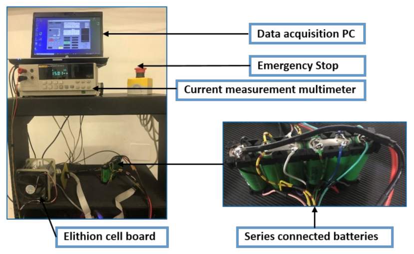
2.1. System Description and Experiment

The system-level application architecture for SOH estimation is shown in Figure 1. Given a load request from the cell, the measured current and the corresponding voltage are acquired from the cell. The SOC and SOE are computed with suitable functions that are embedded in the Battery Management System (BMS). The SOH estimation algorithm is executed periodically with no dependence on the data log of previous estimations. When the algorithm is triggered, the feature extraction algorithm extracts the relative voltage, SOC, and SOE within a buffer of 40 s of time. The discrete instantaneous values of the SOC and SOE are also acquired at this time interval. These contribute to the training features that are given as input to the ANN-based classifier. Considering the slow dynamics of SOH, the algorithm can be triggered on an hourly basis.

The proposed method aims at estimating the SOH of a lithium-ion cell under dynamic varying load conditions. In the present analysis, the SOC and SOE are computed analytically. The analysis is conducted with a single cell in a module consisting of six (6) individual LG MJI 18650 lithium-ion cells of 3500 mAh capacity connected in series. The characteristics of the cells are shown in

Table 1. Nominal characteristics of cylindrical LG 18650 MJ1 lithium-ion cell [37].

Cell Chemistry		LiNiMnCoO2
Nominal capacity (@ 0.2C, 4.2–2.5 V, 23 °C)		3500 mAh
Nominal voltage		3.635 V
Cut-off voltage		2.5 V
Max. discharge current		10 A
Cycle life ([email protected] A, discharge@4 A)		>400 cycles
Charge Condition	Max. current	1 C (3400 mA)
	Max. voltage	4.2 ± 0.05 V
Operating Condition	Charge	0–45 °C
	Discharge	−20–60 °C
Mass		49.0 g
Dimension	Diameter	18.5 mm
	Height	65 mm

. The procedure has been designed for a single cell. The SOH of a battery pack can be developed by series and parallel connection of cells, putting into consideration the capacity variations in the cells and the error introduced by the interconnection resistance [36].

The data used for the experiment were acquired from a test bench that was developed in-house. The test bench shown in Figure 2 consists of six cells connected in a series with the cell voltages measured with Elithion cell boards. Two LM35 Texas Instrument temperature sensors measure the cell surface temperature. An Elithion (Lithulmate) BMS is installed on the test bench to enhance the safety of the acquisition process. An Arduino Mega board was connected via LAN to a dedicated PC and then used to acquire the measured data. As an extra safety measure, the system is equipped with an emergency stop device.

The experiment is conducted in a controlled ambient room temperature condition. The cells are cooled by natural convection with proper air circulation in the room, and the room temperature is unaffected by the heat from the cells. The two temperature sensors are mounted on the surface of the cells to ensure measurement consistency and the information is fed to the BMS for detecting overheating.

To age the cell, a major cycle consisting of seventeen (17) profiles is repeated fourteen times corresponding to about 470 cycles. The load profiles are either charge or discharge phase or a sequence of charge and discharge as in the dynamic load profile. The aging profiles include constant current constant voltage (1.75 A), constant current (0.7 A) discharge, step current (0 A to 4.23 A) charge, constant power discharge, step current (0 A to −10 A) discharge, and dynamic current profile. Each charge or discharge phase is completed with the respective SOC of 100% or 0% and followed by a rest period. The choice of these aging profiles is to create the possibility to validate the cells under different load conditions. The profiles are shown in Figure 3. The entire aging process lasted for about 77 days.

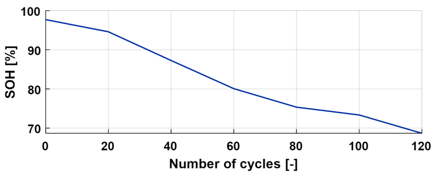
2.2. State of Health (SOH)

The health of a lithium-ion cell is affected by cycle life aging due to usage and calendar aging due to storage time. Since the cell has been cycled until the end of life (EOL) with negligible storage time, the calendar aging is neglected in this work. SOH as a health state index is computed based on the capacity measurement over the cycle life of a cell to account for the capacity fading. When a cell is fully charged, it has a maximum releasable capacity, $C_{max}$. This capacity can change relative to the capacity at the beginning of life, $C_{bol}$, which is assumed to be the maximum capacity of a cell when newly installed. $C_{max}$ decays with storage time and usage of the cell. Such decay over the cell aging cycles can be observed by normalizing the $C_{max}$ at a given cycle with the $C_{bol}$. This represents the SOH [38] as in Equation (1).

$$\mathrm{SOH}=\frac{C_{max}}{C_{bol}}\times 100\%$$

(1)

The experiment for SOH estimation was conducted at room temperature, cycling the cell under different load profiles until the EOL is reached. According to the standard adopted by the automotive industry, the EOL of a cell is reached after 20% capacity fading. Therefore, the useful life of the cell is considered between 100% to 80% SOH [39]. To benchmark the SOH, a constant current discharge profile of 0.7 A (0.2 C) is applied at the intervals between the dynamic profiles to compute across different aging cycles. With such a low C-rate, the internal resistance of the cell is low and the approximate SOH without load stress can be measured. With this current profile, the cell is completely discharged in 238 min during the first cycle when the cell is new. When the cell gets aged, as represented by the last cycle, it gets completely discharged in 166 min. The SOH of the lithium-ion cell is plotted in Figure 4, computed according to Equation (1) for the aging cycles from 100% to 70% SOH.

In the present analysis, SOH is categorized into five (5) classes. Class 1 to Class 4 represent the range of 100% to 80% SOH, where each class corresponds to an interval of a length of 5%. Class 5 represents the SOH below 80%. These classes are measured at the outputs of the classifier algorithm. The conservative interval used in this analysis is within the range of acceptance for similar applications.

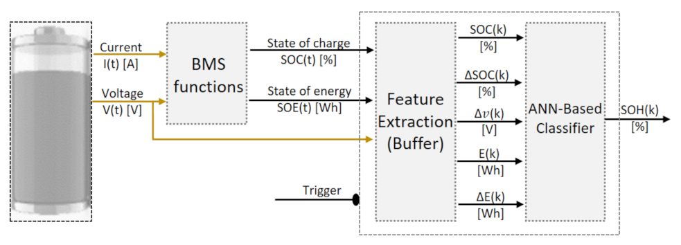
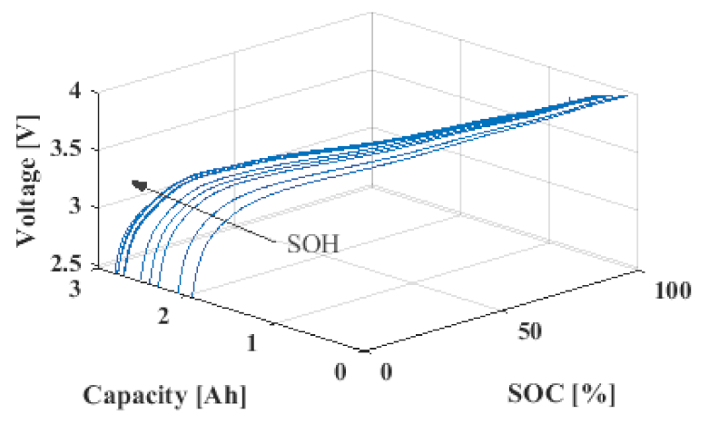
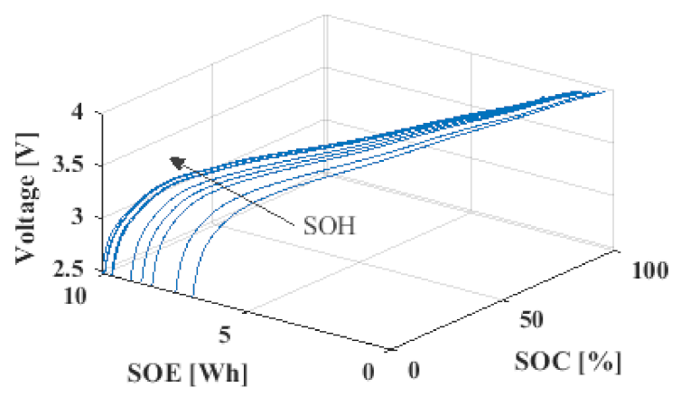
2.3. SOH Characterization and Feature Extraction

Defining the features that influence the cell SOH is very critical. Some useful strategies that are documented in the literature have been reviewed in Section 1. It is shown in this work that SOH can be characterized by some indicators such as voltage [V], SOC [%], and energy [Wh] as listed in

Table 2. Dataset characterization: the input and output of the ANN-based algorithm. The input features are computed on a buffer with a time length of 40 s.

Model Input				Model Output Classes
#	Variable	Feature	Unit	Class	SOH Range [%]
1.	Voltage	$∆v$	[V]	1	100–95
2.	State of charge	SOC	[%]	2	95–90
		ΔSOC	[%]	3	90–85
3.	State of energy	SOE	[Wh]	4	85–80
		ΔSOE	[Wh]	5	<80

. While SOC is the percentage of the ampere-hour (Ah) in the cell, energy is the area under the Ah-voltage curve. These characteristic variables are the parametric variables of the cell that show some significant correlation with cell aging. Clear distinctions exist also on the time variation of these variables, as will be seen subsequently. Although SOH estimation is also influenced by environmental temperature, the analysis here is considered only for room temperature.

Theoretically, the measured terminal voltage is a contribution of open-circuit voltage ($v_{oc}$), polarization voltage ($v_p$), and the ohmic voltage ($v_{ohm}$) according to Equation (2).

$$v\left(t\right)=v_{oc}\left(\mathrm{SOC}\left(t\right)\right)+v_p\left(t\right)+v_{ohm}\left(t\right)$$

(2)

The $v_{oc}$ is the equilibrium voltage and it is a function of SOC. The $v_p$ models the transient of the voltage dynamics. The presence of the $v_{ohm}$ implies that the energy state is not conserved and hence with usage, the energy capacity of the cell reduces and aging occurs. The characterization is shown for a constant discharge current of 0.7 A profile. The cell of 4.2 V maximum voltage is continuously discharged until the minimum cut-off voltage of 2.5 V is reached. Figure 5 shows the SOH characterization based on voltage and capacity.

From Figure 5, it can be seen that as the lithium-ion cell ages, the minimum voltage of the cell is reached quicker during discharge as the cell ages. The degraded capacity results from the consumed active electrode and results in a faster charge and discharge as the cell ages.

The cell SOC is an important parameter upon which many variables and other cell parameters are dependent, and it is defined as the percentage of charge in a cell relative to the maximum cell capacity. Battery SOH is a slow dynamic variable relative to the SOC, and the true value of the SOC is not known except with the knowledge of the value of the SOH. The computation of SOC at implementation will require a knowledge of the SOH that will be applied as a correction parametric variable. SOC is computed with (3). Equation (4) computes the relative state of charge, $∆\mathrm{SOC}$, across a buffer of defined time length $t_b$ with respect to the initial time $t_0$.

$$\mathrm{SOC}\left(t\right)=\mathrm{SOC}\left(t_0\right)+\frac{{\int }_{t_0}^t{\eta }_{c}i\left(t\right)dt}{C_{max}}$$

(3)

$$∆\mathrm{SOC}\left(t\right)=\mathrm{SOC}\left(t_b\right)-\mathrm{SOC}\left(t_0\right)$$

(4)

$C_{max}$ is the maximum capacity of the cell for a given cycle. It is updated at each cycle as the cell ages such that the SOC is always in the range of 0–100%, but the slope varies. The total amount of charge deposited in the cell while charging is often not completely recoverable in the discharge phase [38,40]. The charge phase is weighted with a Coulomb efficiency, ${\eta }_c$, to compensate for this variation. In this work, ${\eta }_c$ of 94% is computed to provide the best fit when the SOH across the cycles for charge and discharge phases are compared. Figure 6 shows that the magnitude of the SOC gradient increases as the cell ages.

The rapid change in voltage at the extreme upper and the lower range of the SOC introduces large nonlinearity that impacts the training result of the classifier. To minimize this effect, the energy variation is taken into consideration. It is computed according to Equation (5) as the integral of voltage and current over time.

$$\mathrm{SOE}\left(t\right)=\underset{t_0}{\overset{t}{{\displaystyle \int }}}{\eta }_{e}v\left(t\right)i\left(t\right)dt$$

(5)

where ${\eta }_e$ is the energy efficiency [40] of 0.88% chosen as the best fit comparison between the maximum absolute SOE distribution across the aging cycles. As in the SOC computation, to compensate for the energy difference between the charge and discharges phases, ${\eta }_e$ is applied as a weighting factor to the computed energy of the charge phase. Figure 7 shows the characterization of SOH based on the cell voltage, SOC, and SOE.

The feature extraction block in Figure 1 consists of a buffer of 40 s time length. The buffer size is chosen as a good compromise to minimize the impact of measurement noise and loss of data points. The relative values of voltage, SOC, and SOE in the buffer are computed at the interval of this buffer length. In addition, the instantaneous value of both SOC and SOE is recorded. The outputs of the feature extraction block are given as input to the classifier. Figure 8 shows the relative values of voltage, SOC, and SOE taken at intervals that correspond to the buffer time length of 40 s. Figure 8a,b show the values against time for the first and last cycle, respectively. As mentioned above, the complete discharge of the cell lasted for 238 min in the first cycle when the cell is new. When aged, in the last cycle, the discharge lasted for 166 min.

Information provided by the feature variables is learned by the classifier during the training. The magnitude of the variation of voltage, SOC, and SOE can be seen to change significantly as the cell ages from the first to the last cycle. The $\mathsf{\Delta }v$ magnitude doubled from the original value of −0.0015 V. The $\mathsf{\Delta }\mathrm{SOC}$ changed from −0.28% to −0.4%. The magnitude of the slope of $\mathsf{\Delta }\mathrm{SOE}$ increased as the cell aged. Additional information is provided by the remaining features, the instantaneous values of SOC and SOE as seen from Figure 7. This information is learned by the neural network classifier to estimate the SOH.

2.4. Design of the Classifier Model

The choice of a classification method for SOH estimation is considered suitable since it eliminates the need of staying consistent with the time history of the cell aging. The architecture of the neural network classifier is shown in Figure 9. The network consists of the input layer, two hidden layers with ten neurons each, and the output layer. The input layer has five (5) neurons that correspond to the number of feature variables, while the output layer has five (5) neurons that correspond to the number of classes. The number and the size of the hidden layers are determined heuristically.

The classifier is designed with a network training function that updates the weights $w$ and bias $b$ values according to Levenberg−Marquardt (trainlm) [41,42]. The Levenberg–Marquardt algorithm is a higher-order adaptive algorithm that minimizes the mean square error (MSE) $e$ of a neural network output layer. To minimize the error, a second-order algorithm uses the Hessian to determine the weight and biases update as in Equation (6). The error gradient $\nabla e\left(\beta \right)$ is computed from Equation (7). Refer to [42] for more information.

$$\underset{\beta }{\min }e\left(\beta \right)=\frac{1}{2}\sum e_i{\left(\beta \right)}^2=\frac{1}{2}e{\left(\beta \right)}^{T}e\left(\beta \right)$$

(6)

$$\nabla e\left(\beta \right)=J{\left(\beta \right)}^{T}e\left(\beta \right)$$

(7)

where $J\left(\beta \right)$ is the Jacobian matrix; $\beta$ is the weight and bias parameters obtained by least squares; $e\left(\beta \right)$is a vector of the sample point errors.

The hidden layer activation function (HAF) is the hyperbolic tangent sigmoid, and the output activation function (OAF) is the softmax function. The parameters of the neural network classifier are reported in

Table 3. Parameters of the neural network classifier.

Parameter	Value
Number of inputs	5
Number outputs	5 classes
Number of hidden layers	2
Number of neurons per hidden layer	10
Performance goal	0
Minimum performance gradient	$1\times {10}^{-20}$
Adaptive factor, mu	0.001
Maximum validation fails	50

.

The classifier model is trained once and the cross-entropy cost function is used to evaluate the performance. The training processes ended after 821 epochs using a personal computer that has an Intel(R) Core(TM) i5-2450M CPU @ 2.50 GHz dual-core processor. The cross-entropy returns a low MSE performance value of 0.01035 based on Equations (6) and (7). The MSE plot is shown in Figure 10.

3. Results and Discussion

The training and validation results are discussed in this section. The classifier is trained with the dynamic load profile whose maximum current amplitude is 5 A in both charge and discharge phases. At room temperature, the model is validated with the dynamic load profile, a constant load profile, and a step load profile. Finally, the model is validated for applicability in multiple cells under dynamic load conditions.

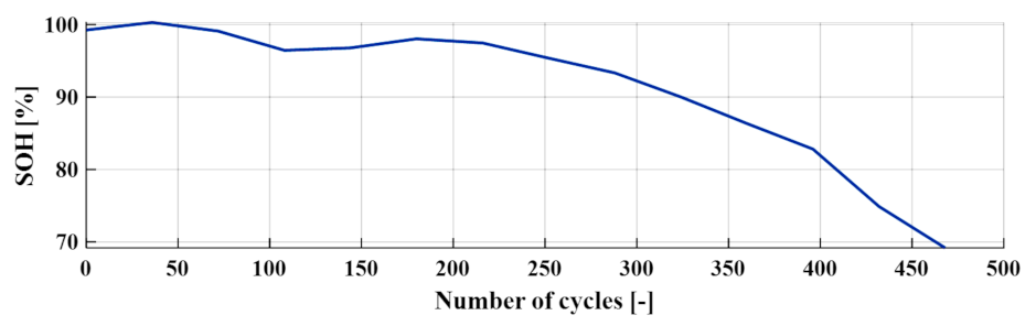
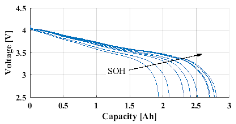
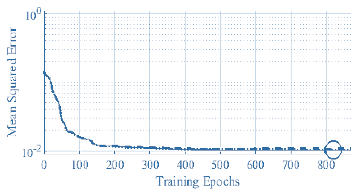
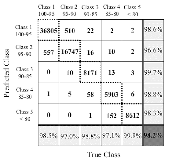
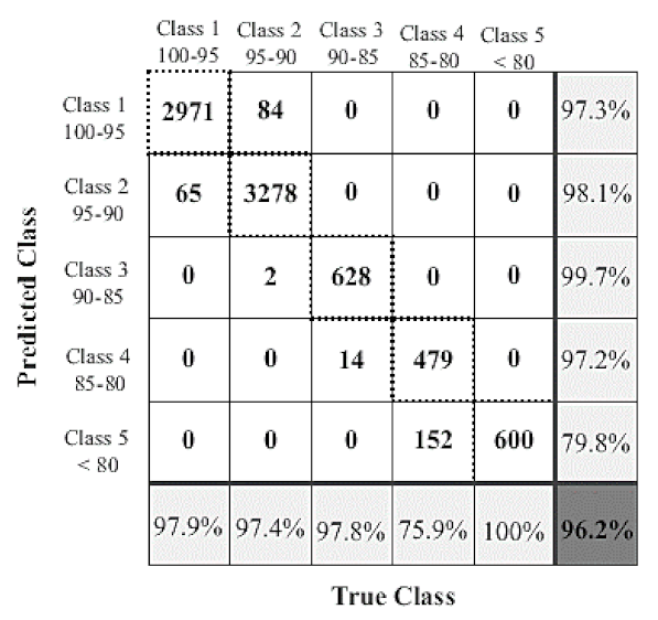
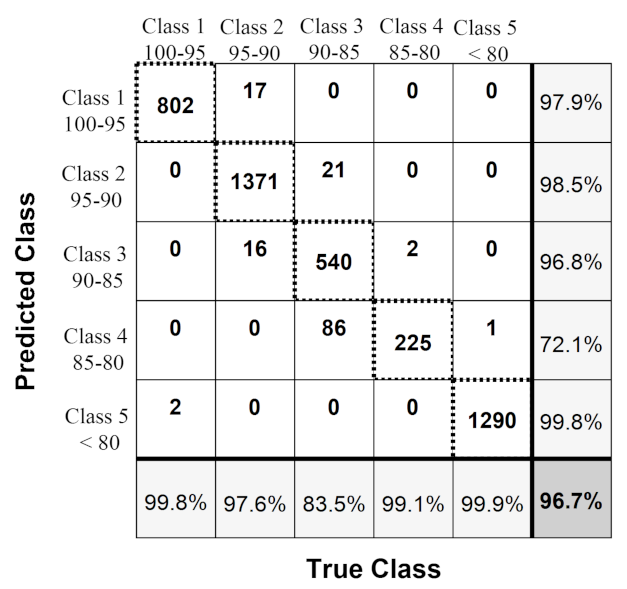
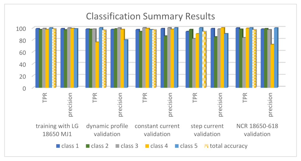
3.1. Training and Validation with the Dynamic Load Profile

The dynamic load profile consists of a total number of 130 profiles, of which 118 profiles are used for the training while the rest are used for the validation. Figure 11 shows the first two dynamic load profiles of the aging cycles used in model training and validation.

The measured voltage of the dynamic varying load profile is corrupted by some high-frequency noise of the order of 2 mV and irregular spikes of up to 80 mV that results from a rapid change of the load input. To avoid the impact of this noise on the classifier, the measured voltage data is smoothened using the moving average function with a smoothing factor of 0.01.

The training dataset consists of the $X\left(n\right) \in {\mathcal{R}}^{5\times N}$ feature variables and $Y\left(n\right) \in {\mathcal{R}}^{5\times N}$ output. The matrix rows correspond to the five (5) features and the five (5) classes, respectively. $N$ corresponds to the number of training data points, which is the number of buffers. The original dataset is sampled at a 1 s rate, while the buffer has a time length of 40 s. Some information may be lost in the long timespan between the buffer intervals. Furthermore, the initial SOC of a cell may vary in practice. Considering these limitations, the model can be enhanced during the training by repeating each aging cycle with a moving window that is shifted at an interval of 10 s.

The 118 dynamic profiles were used for the training and that corresponds to 77,608 buffers and 90% of the entire buffers extracted from the profile. The dynamic profiles used for the training and validation consists of profiles polarized to either charge or discharge the cell for a given cycle.

The training and validation results are analyzed with the help of the confusion matrix. Figure 12 shows the confusion matrix of the trained model. The columns of the matrix are the five (5) target or true classes. The rows are the predicted classes. The diagonal cell corresponds to the buffers that are correctly classified. The off-diagonal cells are the misclassified buffers. The number of observations is shown in each cell. The last column shows the precision of prediction per class. In other words, it shows the percentage of consistency of prediction with the true value for each class. The last row shows the percentage of each class that is correctly classified. This is also known as the true positive rate, TPR. The total accuracy is shown at the bottom-right cell. The accuracy of the model in the training phase is 98.2%. This corresponds to an error of 1.8%, which is equivalent to 1370 misclassified buffers over 77,608 total training buffers.

After training the model, the model is validated with buffers from dynamic profiles that the trained model has not yet seen. To do this, the remaining 12 profiles corresponding to 10% of the entire buffers are given as inputs to the trained model. The dynamic load profile data as in the training has a maximum current amplitude of 5 A. The performance of the model is then analyzed with a confusion matrix as in Figure 13. The accuracy of the model in the validation phase is 96.2% and results in a total number of 317 misclassified buffers over 8273 buffers.

From Figure 12, it can be seen that the TPR of the classifier at validation is considerably high and in the range of 76% to 100%. Moreover, the model precision is in the range of 80% to 99.7%.

3.2. Validation with the Constant Current Constant Voltage (CCCV) Load Profile

The constant current validation is performed with a CCCV load profile. The cell is charged with a constant current of 1.75 A until the voltage reaches about 3.8. The constant voltage mode is then activated until the minimum current of 0.3 A is reached. The consideration of this profile is relevant to provide validation of the model for constant current applications such as in the charging model of the plug-in electric vehicle. A CCCV profile of the first aging cycle is shown in Figure 14.

The constant current profile consists of 12 charge cycles whose features are extracted in 5879 buffers. The model performance under constant current charge condition is shown in Figure 15 with a confusion matrix.

The accuracy of the classifier under constant current charge condition is 96.6% with 197 buffers misclassified over 5879 total buffers. TPR is in the range of 93.7% to 98.9%, while the precision is in the range of 86.2% to 100%. No buffer is in Class 3.

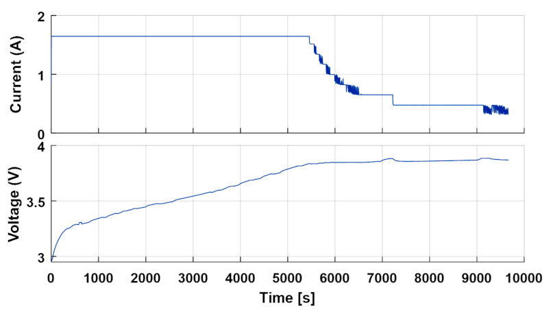
3.3. Validation with the Step Load Profile

Here the step current profile is applied to validate the model for aggressive applications. The step current changes at the 0.47 A interval in the range of 0–4.23 A. The step current profile consists of 11 cyclic charge profiles captured within 2700 buffers. The profile with the corresponding voltage is shown in Figure 16.

The confusion matrix-based performance of the classifier under step current charge condition is shown in Figure 17. The accuracy of the classifier under step current charge condition is 93.8% with 163 buffers misclassified over 2700 total buffers. TPR is in the range of 82% to 100%, while the precision is in the range of 84.8% to 100%.

The validation with the step current profile represents a relatively aggressive validation with respect to the other profiles. For this reason, relatively lower performance is acceptable.

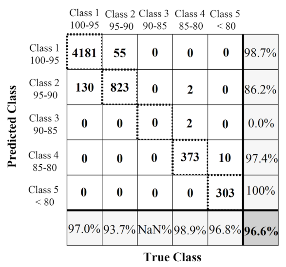
3.4. Validation with New Cell

The final validation of the model is performed with an entirely new cell of slightly similar specification. The experiment and analysis performed above are repeated for a Sanyo NCR 18650 GA Lithium cell. Although the Sanyo NCR cell shares a similar specification with the LG MJ1, their chemistries are different. Information about the cell is given in

Table 4. Nominal characteristics of cylindrical Sanyo NCR 18650 GA lithium-ion cell [43].

Cell Chemistry		LiNiCoAlO2
Nominal capacity (@ 0.2 C, 4.2–2.5 V, 25 °C)		3300 mA
Nominal voltage		3.6 V
Cut-off voltage		2.5 V
Max. discharge current		10 A
Cycle life ([email protected] A, discharge@4 A)		>300 cycles
Charge Condition	Max. current	1 C (3350 mA)
	Max. voltage	4.2 ± 0.03 V
Operating Condition	Charge	0–40 °C
	Discharge	−20–60 °C
Mass		49.0 g
Dimension	Diameter	18 mm
	Height	65 mm

.

The cell is aged in a similar procedure as demonstrated earlier with similar load profiles in a repeated pattern. The cell reached the SOH of about 70% after about 120 cycles. The SOH of the cell across the aging cycle is shown in Figure 18.

To extract the feature variable data for validating the neural network, the ${\eta }_c$ and ${\eta }_e$ are computed as 0.91 and 0.83, respectively, to obtain the best fit between the charge and discharge SOH across the aging cycles. This stage of validation applies only the dynamic load profile shown in Figure 10. The feature variables are then computed as described earlier and applied as input to the trained classifier. The model performance is again analyzed with a confusion matrix as in Figure 19. A total number of 4371 buffers are extracted from the polarized dynamic load profile. About 4228 of the buffers are correctly classified while 143 buffers are wrongly classified. This results in 96.7% total accuracy of the model.

These results of the training and the various validations of the classifier model are summarized in Figure 20, including information on the model precision, the TPR, and the total accuracy.

To compare the proposed model with the state of the art, it was observed that only a few authors have reported the SOH estimation under dynamic load conditions employing classification. Ref. [26] reported the estimation of SOH under such conditions using a similar classification approach. However, SOH was estimated only in the dynamic discharge modes, hence resulting in a conservative model with an accuracy of 97.5%. In the proposed model, the accuracy of 96.2% is obtained for the model validation with dynamic profiles according to Figure 11.

The classifier is designed, trained, and validated with MATLAB/Simulink 2020b equipped with a Neural network toolbox. After the training and validation, the trained classifier is deployed to a Texas F28379D microcontroller unit (MCU) target. The real-time execution speed is estimated by a processor-in-the-loop simulation to verify the model for online applicability. Given some sampling points of the feature variables as input from Simulink software, the model is simulated in the MCU. The model execution speed is verified as 8.34 µs in real time and with a negligible CPU occupation. In comparison, the PL-ELM performs a similar operation by regression with an execution speed of 93 µs [28]. In the real implementation, the classification algorithm is periodically triggered to extract the feature variables of the classifier in the buffer using information from an installed battery. These features are then applied as input to the trained classifier for predicting the battery SOH.

4. Conclusions and Recommendation

Analysis of battery SOH under dynamic load conditions is essential for the design of a high-fidelity estimation model. This, however, has been sparingly addressed in the literature. In this work, the SOH of a lithium-ion cell is analyzed and estimated under dynamic load conditions implementing an ANN-based classifier. This approach minimizes the time history dependency and the need for continuous initialization of the model.

The SOH is experimentally characterized by the cell’s voltage, SOC, and SOE at room temperature. An ANN-based classifier model is trained using features that are extracted from the characterizing variables. These features include the instantaneous values of SOC and SOE, and the relative values of voltage, SOC, and SOE across the buffer of a defined time length.

The trained model is validated for application under different scenarios, including dynamic load conditions, constant load conditions, and step load conditions. The performance of the resulting validated model is analyzed with matrices, and the accuracy of the model is 96.2%, 96.6%, and 93.8% for the respective load conditions. The model is further validated for use on other cells that have similar specifications. The results show that an accuracy of 96.7% is possible under dynamic load conditions.

Finally, the model is validated for online applicability through processor-in-the-loop simulation. An average execution time of 8.34 µs and a negligible CPU occupation of the algorithm is verified with a Texas F28379D microcontroller unit (MCU) board. This makes the model suitable for online automotive applications where computational resources impose a constraint.

For future work, it was noticed that the model poorly classifies buffers whose SOHs are very close to the boundary of two classes. For instance, buffers whose true SOHs are close to 95% (say 95.01%) may partly be misclassified as Class 2. Improving the precision of the model for such cases will be the focus of future work. Secondly, the classifier will be validated for application under a wider range of temperature conditions.

SOH is impacted by temperature. However, this model is validated only at ambient room temperature. This limits its application for only such a condition. It will be of useful research interest to further validate the model over different temperatures.

References

1. Liu, R.; Zhang, C. An Active Balancing Method Based on SOC and Capacitance for Lithium-Ion Batteries in Electric Vehicles. Front. Energy Res. 2021, 9, 662. [Google Scholar] [CrossRef]
2. Yakhshilikova, G.; Ezemobi, E.; Ruzimov, S.; Tonoli, A. Battery Sizing for Mild P2 HEVs Considering the Battery Pack Thermal Limitations. Appl. Sci. 2022, 12, 226. [Google Scholar] [CrossRef]
3. Vetter, J.; Novák, P.; Wagner, M.R.; Veit, C.; Möller, K.-C.; Besenhard, J.O.; Winter, M.; Wohlfahrt-Mehrens, M.; Vogler, C.; Hammouche, A. Ageing Mechanisms in Lithium-Ion Batteries. J. Power Sources 2005, 147, 269–281. [Google Scholar] [CrossRef]
4. Ma, G.; Zhang, Y.; Cheng, C.; Zhou, B.; Hu, P.; Yuan, Y. Remaining Useful Life Prediction of Lithium-Ion Batteries Based on False Nearest Neighbors and a Hybrid Neural Network. Appl. Energy 2019, 253, 113626. [Google Scholar] [CrossRef]
5. Jia, J.; Liang, J.; Shi, Y.; Wen, J.; Pang, X.; Zeng, J. SOH and RUL Prediction of Lithium-Ion Batteries Based on Gaussian Process Regression with Indirect Health Indicators. Energies 2020, 13, 375. [Google Scholar] [CrossRef] [Green Version]
6. Wang, K.; Gao, F.; Zhu, Y.; Liu, H.; Qi, C.; Yang, K.; Jiao, Q. Internal Resistance and Heat Generation of Soft Package Li4Ti5O12 Battery during Charge and Discharge. Energy 2018, 149, 364–374. [Google Scholar] [CrossRef]
7. Wei, X.; Zhu, B.; Xu, W. Internal Resistance Identification in Vehicle Power Lithium-Ion Battery and Application in Lifetime Evaluation. In Proceedings of the 2009 International Conference on Measuring Technology and Mechatronics Automation, Zhangjiajie, China, 11–12 April 2009; Volume 3, pp. 388–392. [Google Scholar]
8. Sajfar, I.; Malaric, M.; Bullough, R.P. Sealed Batteries in Transient Limiting Distribution Networks-Methods of Measuring Their Internal Resistance. In Proceedings of the 12th International Conference on Telecommunications Energy, Orlando, FL, USA, 21–25 October 1990; pp. 458–463. [Google Scholar]
9. Schweiger, H.-G.; Obeidi, O.; Komesker, O.; Raschke, A.; Schiemann, M.; Zehner, C.; Gehnen, M.; Keller, M.; Birke, P. Comparison of Several Methods for Determining the Internal Resistance of Lithium Ion Cells. Sensors 2010, 10, 5604–5625. [Google Scholar] [CrossRef] [PubMed] [Green Version]
10. Piłatowicz, G.; Marongiu, A.; Drillkens, J.; Sinhuber, P.; Sauer, D.U. A Critical Overview of Definitions and Determination Techniques of the Internal Resistance Using Lithium-Ion, Lead-Acid, Nickel Metal-Hydride Batteries and Electrochemical Double-Layer Capacitors as Examples. J. Power Sources 2015, 296, 365–376. [Google Scholar] [CrossRef]
11. He, J.; Wei, Z.; Bian, X.; Yan, F. State-of-Health Estimation of Lithium-Ion Batteries Using Incremental Capacity Analysis Based on Voltage–Capacity Model. IEEE Trans. Transp. Electrif. 2020, 6, 417–426. [Google Scholar] [CrossRef]
12. Guha, A.; Patra, A. State of Health Estimation of Lithium-Ion Batteries Using Capacity Fade and Internal Resistance Growth Models. IEEE Trans. Transp. Electrif. 2018, 4, 135–146. [Google Scholar] [CrossRef]
13. Lashway, C.R.; Mohammed, O.A. Adaptive Battery Management and Parameter Estimation Through Physics-Based Modeling and Experimental Verification. IEEE Trans. Transp. Electrif. 2016, 2, 454–464. [Google Scholar] [CrossRef]
14. A New Method for State of Charge and Capacity Estimation of Lithium-Ion Battery Based on Dual Strong Tracking Adaptive H Infinity Filter. Available online: https://www.hindawi.com/journals/mpe/2018/5218205/ (accessed on 3 January 2022).
15. A Multi-Timescale Estimator for Battery State of Charge and Capacity Dual Estimation Based on an Online Identified Model-ScienceDirect. Available online: https://www.sciencedirect.com/science/article/pii/S030626191730140X?via%3Dihub (accessed on 3 January 2022).
16. Azis, N.A.; Joelianto, E.; Widyotriatmo, A. State of Charge (SoC) and State of Health (SoH) Estimation of Lithium-Ion Battery Using Dual Extended Kalman Filter Based on Polynomial Battery Model. In Proceedings of the 2019 6th International Conference on Instrumentation, Control and Automation (ICA), Bandung, Indonesia, 31 July–2 August 2019; pp. 88–93. [Google Scholar]
17. Fang, L.; Li, J.; Peng, B. Online Estimation and Error Analysis of Both SOC and SOH of Lithium-Ion Battery Based on DEKF Method. Energy Procedia 2019, 158, 3008–3013. [Google Scholar] [CrossRef]
18. Tang, X.; Liu, K.; Wang, X.; Liu, B.; Gao, F.; Widanage, W.D. Real-Time Aging Trajectory Prediction Using a Base Model-Oriented Gradient-Correction Particle Filter for Lithium-Ion Batteries. J. Power Sources 2019, 440, 227118. [Google Scholar] [CrossRef]
19. Tan, X.; Tan, Y.; Zhan, D.; Yu, Z.; Fan, Y.; Qiu, J.; Li, J. Real-Time State-of-Health Estimation of Lithium-Ion Batteries Based on the Equivalent Internal Resistance. IEEE Access 2020, 8, 56811–56822. [Google Scholar] [CrossRef]
20. Singh, P.; Kaneria, S.; Broadhead, J.; Wang, X.; Burdick, J. Fuzzy Logic Estimation of SOH of 125Ah VRLA Batteries. In Proceedings of the INTELEC 2004. 26th Annual International Telecommunications Energy Conference, Chicago, IL, USA, 19–23 September 2004; pp. 524–531. [Google Scholar]
21. Bian, X.; Wei, Z.; Li, W.; Pou, J.; Sauer, D.U.; Liu, L. State-of-Health Estimation of Lithium-Ion Batteries by Fusing an Open Circuit Voltage Model and Incremental Capacity Analysis. IEEE Trans. Power Electron. 2022, 37, 2226–2236. [Google Scholar] [CrossRef]
22. Kim, J.; Yu, J.; Kim, M.; Kim, K.; Han, S. Estimation of Li-Ion Battery State of Health Based on Multilayer Perceptron: As an EV Application. IFAC-PapersOnLine 2018, 51, 392–397. [Google Scholar] [CrossRef]
23. Noura, N.; Boulon, L.; Jemeï, S. A Review of Battery State of Health Estimation Methods: Hybrid Electric Vehicle Challenges. World Electr. Veh. J. 2020, 11, 66. [Google Scholar] [CrossRef]
24. Wang, Z.; Feng, G.; Zhen, D.; Gu, F.; Ball, A. A Review on Online State of Charge and State of Health Estimation for Lithium-Ion Batteries in Electric Vehicles. Energy Rep. 2021, 7, 5141–5161. [Google Scholar] [CrossRef]
25. Sarmah, S.B.; Kalita, P.; Garg, A.; Niu, X.; Zhang, X.-W.; Peng, X.; Bhattacharjee, D. A Review of State of Health Estimation of Energy Storage Systems: Challenges and Possible Solutions for Futuristic Applications of Li-Ion Battery Packs in Electric Vehicles. J. Electrochem. Energy Convers. Storage 2019, 16. [Google Scholar] [CrossRef] [Green Version]
26. Bonfitto, A. A Method for the Combined Estimation of Battery State of Charge and State of Health Based on Artificial Neural Networks. Energies 2020, 13, 2548. [Google Scholar] [CrossRef]
27. Bonfitto, A.; Ezemobi, E.; Amati, N.; Feraco, S.; Tonoli, A.; Hegde, S. State of Health Estimation of Lithium Batteries for Automotive Applications with Artificial Neural Networks. In Proceedings of the 2019 AEIT International Conference of Electrical and Electronic Technologies for Automotive (AEIT AUTOMOTIVE), Torino, Italy, 2–4 July 2019; pp. 1–5. [Google Scholar]
28. Ezemobi, E.; Tonoli, A.; Silvagni, M. Battery State of Health Estimation with Improved Generalization Using Parallel Layer Extreme Learning Machine. Energies 2021, 14, 2243. [Google Scholar] [CrossRef]
29. Ruan, H.; He, H.; Wei, Z.; Quan, Z.; Li, Y. State of Health Estimation of Lithium-Ion Battery Based on Constant-Voltage Charging Reconstruction. IEEE J. Emerg. Sel. Top. Power Electron. 2021, 1. [Google Scholar] [CrossRef]
30. Jia, B.; Guan, Y.; Wu, L. A State of Health Estimation Framework for Lithium-Ion Batteries Using Transfer Components Analysis. Energies 2019, 12, 2524. [Google Scholar] [CrossRef] [Green Version]
31. Synchronous Estimation of State of Health and Remaining Useful Lifetime for Lithium-Ion Battery Using the Incremental Capacity and Artificial Neural Networks-ScienceDirect. Available online: https://www.sciencedirect.com/science/article/pii/S2352152X19307340?via%3Dihub (accessed on 3 January 2022).
32. Bian, X.; Wei, Z.; He, J.; Yan, F.; Liu, L. A Novel Model-Based Voltage Construction Method for Robust State-of-Health Estimation of Lithium-Ion Batteries. IEEE Trans. Ind. Electron. 2021, 68, 12173–12184. [Google Scholar] [CrossRef]
33. Capacity-Fading Prediction of Lithium-Ion Batteries Based on Discharge Curves Analysis-ScienceDirect. Available online: https://www.sciencedirect.com/science/article/pii/S0378775311015199?via%3Dihub (accessed on 3 January 2022).
34. Estimation of Battery State of Health Using Back Propagation Neural Network—Computer Aided Drafting, Design and Manufacturing. 2014. Available online: https://www.cnki.com.cn/Article/CJFDTotal-CADD201401011.htm (accessed on 3 January 2022).
35. Venugopal, P. State-of-Health Estimation of Li-Ion Batteries in Electric Vehicle Using IndRNN under Variable Load Condition. Energies 2019, 12, 4338. [Google Scholar] [CrossRef] [Green Version]
36. Diao, W.; Jiang, J.; Zhang, C.; Liang, H.; Pecht, M. Energy State of Health Estimation for Battery Packs Based on the Degradation and Inconsistency. Energy Procedia 2017, 142, 3578–3583. [Google Scholar] [CrossRef]
37. Yoido-Dong Youngdungpo-Gu. Specification for LG 18650 MJ1. Available online: https://www.nkon.nl/sk/k/Specification%20INR18650MJ1%2022.08.2014.pdf (accessed on 11 January 2022).
38. Wang, W.; Wei, X.; Choi, D.; Lu, X.; Yang, G.; Sun, C. Chapter 1 - Electrochemical Cells for Medium- and Large-Scale Energy Storage: Fundamentals. In Advances in Batteries for Medium and Large-Scale Energy Storage; Menictas, C., Skyllas-Kazacos, M., Lim, T.M., Eds.; Woodhead Publishing Series in Energy; Woodhead Publishing: Sawston, UK, 2015; pp. 3–28. ISBN 978-1-78242-013-2. [Google Scholar]
39. D6.7 – Battery Management System Standard. Available online: https://Everlasting-Project.Eu/Wp-Content/Uploads/2019/10/EVERLASTING_D6.7_final_20191001.Pdf (accessed on 11 January 2022).
40. Dahbi, M.; Komaba, S. Chapter 16 - Fluorine Chemistry for Negative Electrode in Sodium and Lithium Ion Batteries. In Advanced Fluoride-Based Materials for Energy Conversion; Nakajima, T., Groult, H., Eds.; Elsevier: Amsterdam, The Netherlands, 2015; pp. 387–414. ISBN 978-0-12-800679-5. [Google Scholar]
41. Sapna, S. Backpropagation Learning Algorithm Based on Levenberg Marquardt Algorithm. In Proceedings of the Computer Science & Information Technology (CS & IT), Chennai, India, 31 October 2012; Academy & Industry Research Collaboration Center (AIRCC): Chennai, India; pp. 393–398. [Google Scholar]
42. Khan, N.; Gaurav, D.; Kandl, T. Performance Evaluation of Levenberg-Marquardt Technique in Error Reduction for Diabetes Condition Classification. Procedia Comput. Sci. 2013, 18, 2629–2637. [Google Scholar] [CrossRef] [Green Version]
43. Datasheet Specs for Panasonic Sanyo 18650 Battery. Available online: https://www.orbtronic.com/content/Datasheet-specs-Sanyo-Panasonic-NCR18650GA-3500mah.pdf (accessed on 11 January 2022).
Figure 1. Architecture for SOH estimation using ANN-based classifier. The yellow signals are measurements from the cell.
Energies 15 01234 g001
Figure 2. Experimental setup for data acquisition from lithium-ion batteries connected in series.
Energies 15 01234 g002
Figure 3. Characteristics of the major profiles used for cell aging. (a) constant current (1.75 A) constant voltage charge; (b) constant current (0.7 A) discharge; (c) step current (0 A to 4.23 A) charge; (d) pack constant power discharge (75 W); (e) step current (0 A to −10 A) discharge; (f) dynamic current profile.
Energies 15 01234 g003
Figure 4. SOH of cylindrical LG MJI 18650 lithium-ion cell across the aging cycles.
Energies 15 01234 g004
Figure 5. Characterization of the SOH based on cell voltage and capacity at ambient temperature.
Energies 15 01234 g005
Figure 6. Characterization of the SOH based on the cell voltage and SOC, and capacity at ambient temperature.
Energies 15 01234 g006
Figure 7. Characterization of the SOH based on the cell voltage and SOC, and SOE at ambient temperature.
Energies 15 01234 g007
Figure 8. Feature extraction across buffer of time length of 40 s. (a) Relative values of voltage, SOC, and SOE in the first cycle. (b) Relative values of voltage, SOC, and SOE in the last cycle.
Energies 15 01234 g008
Figure 9. Architecture for pattern recognition feed-forward artificial neural network (ANN) for SOH classification. x(n): input; w: weight of layer neurons; b: bias of the layers; HAF: hidden layer activation function; OAF: output layer activation function.
Energies 15 01234 g009
Figure 10. Mean square error performance result for ANN-based classifier training using Levenberg–Marquardt function.
Energies 15 01234 g010
Figure 11. First-two dynamic load profiles of the aging cycles applied for model training and validation.
Energies 15 01234 g011
Figure 12. Confusion matrix for performance analysis of ANN-based classifier in the dataset trained with LG 18650 MJ1 lithium-ion. The diagonal cells are correctly classified buffers. The last row with gray background is the TPR. The last column with gray background is the precision per class. The bottom right cell with dark background is the total accuracy.
Energies 15 01234 g012
Figure 13. Confusion matrix for performance analysis of ANN-based classifier under dynamic changing load profile validation. The diagonal cells are correctly classified buffers. The last row with gray background is the TPR. The last column with gray background is the precision per class. The bottom right cell with dark background is the total accuracy.
Energies 15 01234 g013
Figure 14. Samples of constant load profile and the voltage used for model validation.
Energies 15 01234 g014
Figure 15. Confusion matrix for performance analysis of ANN-based classifier under constant charge current profile validation. The diagonal cells are correctly classified buffers. The last row with gray background is the TPR. The last column with gray background is the precision per class. The bottom right cell with dark background is the total accuracy.
Energies 15 01234 g015
Figure 16. Sample of step charge current profile and the voltage used for model validation.
Energies 15 01234 g016
Figure 17. Confusion matrix for performance analysis of ANN-based classifier under the step charging current profile validation. The diagonal cells are correctly classified buffers. The last row with gray background is the TPR. The last column with gray background is the precision per class. The bottom right cell with dark background is the total accuracy.
Energies 15 01234 g017
Figure 18. SOH of cylindrical Sanyo NCR 18650 GA lithium-ion cell across the aging cycles.
Energies 15 01234 g018
Figure 19. Confusion matrix for model validation with NCR 18650 GA lithium-ion cell under dynamic load profile. The diagonal cells are correctly classified buffers. The last row with gray background is the TPR. The last column with gray background is the precision per class. The bottom right cell with dark background is the total accuracy.
Energies 15 01234 g019
Figure 20. Result summary of the training and validation of the classifier indicating the TPR, precision per class, and the total accuracy of the classifier according to the confusion matrices.
Energies 15 01234 g020