
Fatigue Strength Analysis of a Prototype Francis Turbine in a Multilevel Lifetime Assessment Procedure Part I: Background, Theory and Assessment Procedure Development

 ,
,
Abstract
:1. Introduction
- Change in the energy mix
- Changes in the operation of hydropower plants due to the new realities
- Changes in the development and expansion of digitalisation
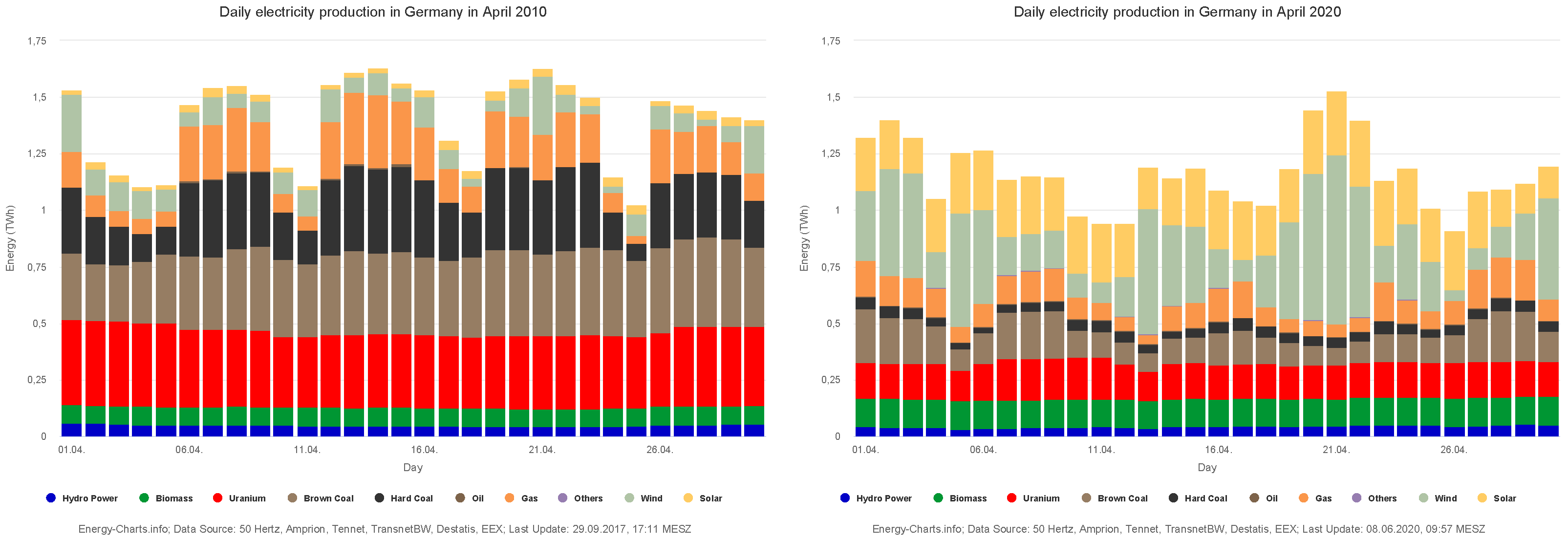
1.1. Change in the Energy Mix
1.2. Changes in the Operation of Hydropower Plants Due to the New Realities
1.2.1. Base Load Electricity Production
1.2.2. Grid Control Operation
- Taking positive and negative balancing power into account, pumped storage plants equipped with two machine-setup units or ternary units are preferable. Only those units can deliver the needed services.
- In terms of mFRR, hydropower plants are one possible resource among others. Start-up of the machine within 5 min and supply of full power by 15 min is achievable for all machine units regardless of age and condition. Even the auxiliary units do not have to be ready for operation and start from a standstill. First, the oil–hydraulic unit must be activated to provide the oil pressure for the auxiliary systems. After that, the turbine shut-off valve is opened, which takes a considerable amount of time to start a hydraulic machine. Only then can the guide vane or the nozzle needle be adjusted and the runner set in rotation. The acceleration of the runner to synchronous speed takes place very quickly. Standard start-up times for Francis turbines require 4–5 min. Pelton turbines can start even faster.
- If pumped storage units are used for secondary control (aFRR), specific prerequisites are already necessary. For example, it is no longer possible to start the machine unit from a standstill in 30 s. Here, at least the turbine shut-off device must already be open and the oil–hydraulic unit pressurized. Only the guide apparatus or the nozzle needle have to be adjusted to synchronize the machine unit with the grid during this period. Power consumption or supply within 5 min is no longer a significant challenge after that. If the start-up time of 30 s is still not achievable under these circumstances, the unit could also remain in standby mode. However, this causes more wear and tear. For aFRR, both types, pump turbines and ternary machine sets, can be used.
- In primary control (FCR), only ternary pumped storage units can be used due to positive and negative power requirements. Conventional pump turbines take too long to switch from the turbine to pump mode. Switchover times of 5–6 min are not uncommon. To react to grid frequency at the crucial period, even the ternary machine sets have to run synchronized on the grid and only shift the load. For the changeover from supply to consumption mode, the machine set must be equipped additionally with a hydraulic shortcut circuit, as otherwise, the changeover time would take too long. Since the machine set must already be running to react in the required time, the pure demand rate is probably not economically sufficient.
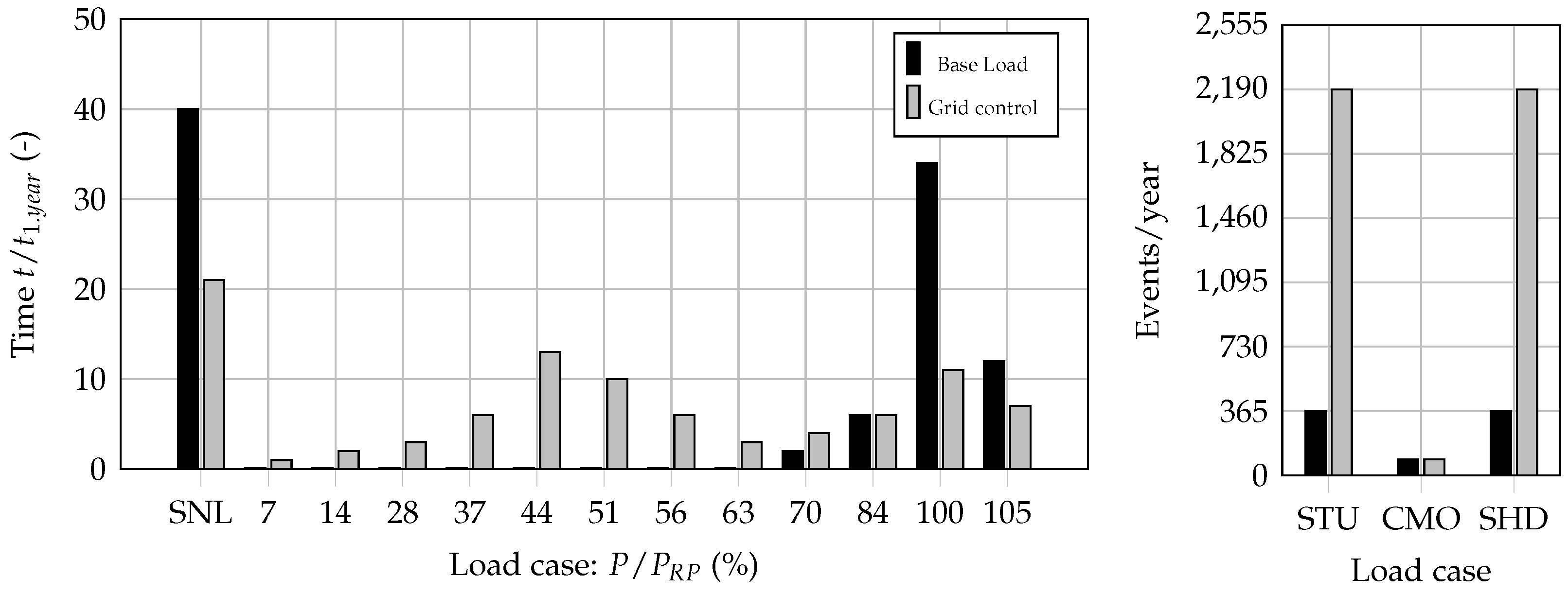
1.2.3. Comparison between Base Load Production and Grid Control Operation
- In base-load electricity production, the machine runs predominantly at its optimum. Therefore, the number of starts and stops of the machine set per day is also lower. In Figure 5, the number of starts and stops per day was set to one, which means that the machine set is started up once a day and remains at the optimum operating point. If the power demand from the grid is deficient, the machine set is left in a synchronized state (SNL) and rotates in “idle mode” in order to be quickly brought back to the optimum and to be able to deliver power when needed.
- In contrast, the machine unit in grid-control mode (aFRR, mFRR) is started and stopped up to six times a day. This is also caused by the purchase of balancing energy on the electricity market in quarter-hour cycles. The machine unit is increasingly operated in the hydraulically unfavorable partial load range, and it is also started and stopped more often than conventionally planned. This results in the high number of start-ups (STU) and shut-downs (SHD) in Figure 5.
- Since the frequency containment reserve (FCR) is primarily intended to mitigate short-term load changes, the entire capacity range has to be provided within a maximum of 30 s and remain continuously available for at least 15 min. This operation means synchronized machine unit and load shifting either from speed-no-load (SNL) point to full load or part load to full load. Additionally, change over from supply to consumption mode is part of this operational field. Start and stops of the machine are less important than faster load shifts and part load operation.
- On the one hand, condenser-mode operation (CMO) only affects machines equipped for such operation, and on the other hand, it is only required for reactive power compensation in the grid. The new renewable energy sources are indeed steadily reducing the reactive power in the grid. However, there are still enough large synchronous generators of the grid’s primary energy suppliers to compensate for this. Hydropower generators can take over this task to some extent. The number of condenser mode operations (CMO) was set at the same low level for the remaining considerations.
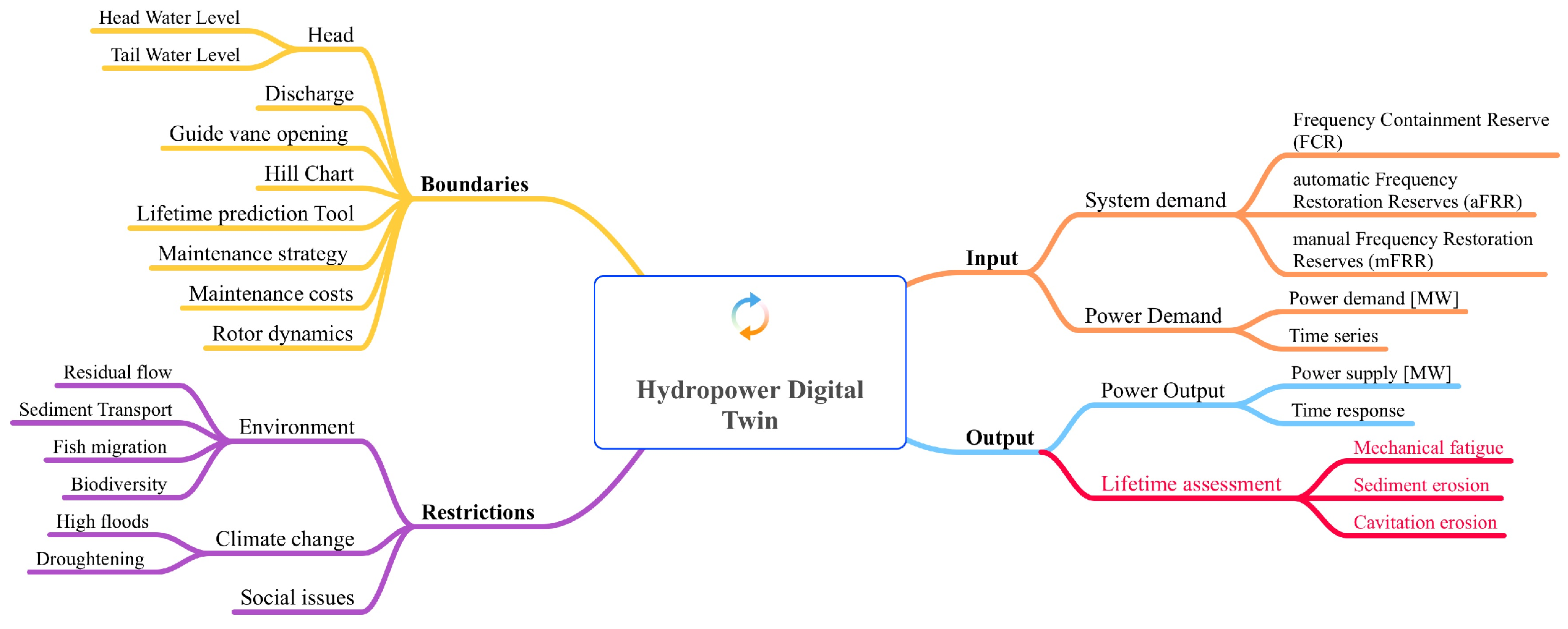
1.3. Changes in the Development and Expansion of Digitalisation
1.3.1. Data Collection
1.3.2. Real-Time Lifetime Prediction
2. Background and Theory
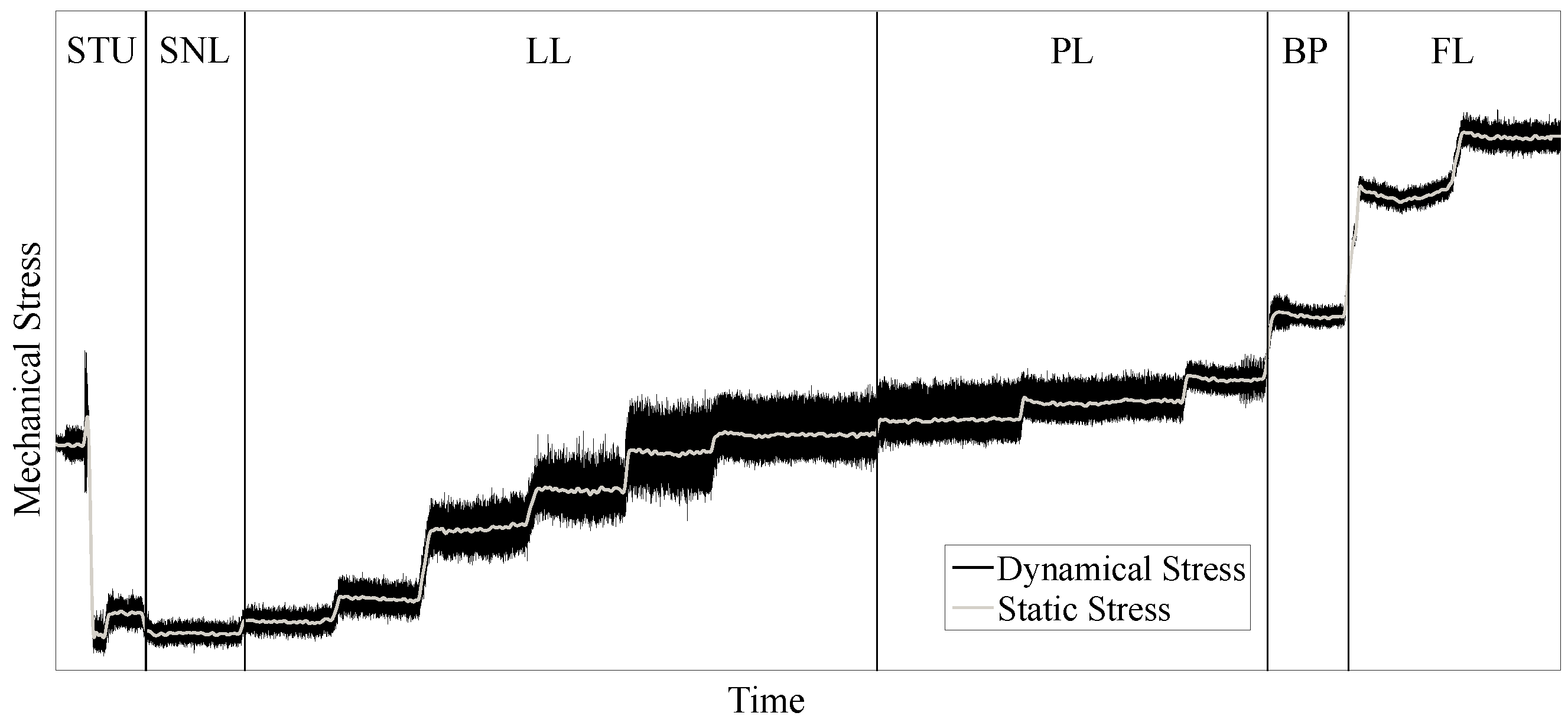
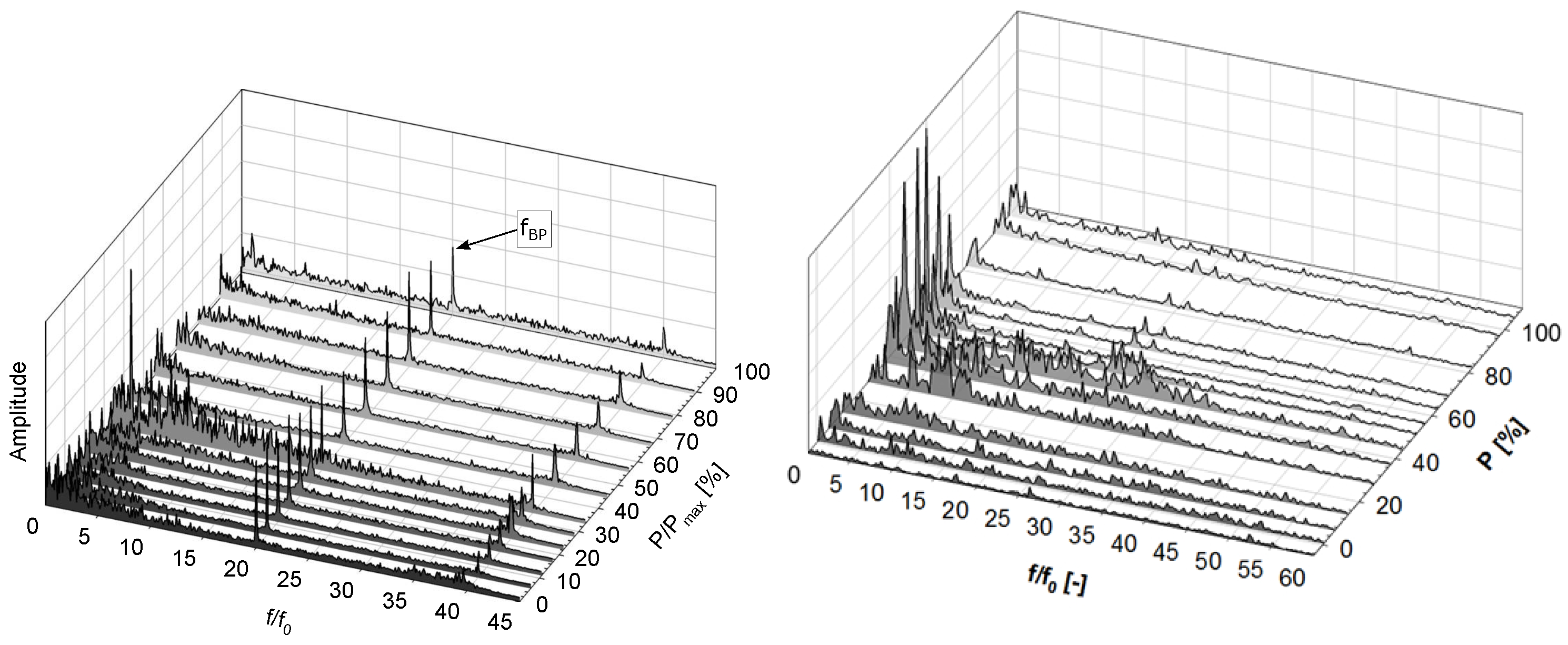
2.1. Stress–Time Correlation at the Runner
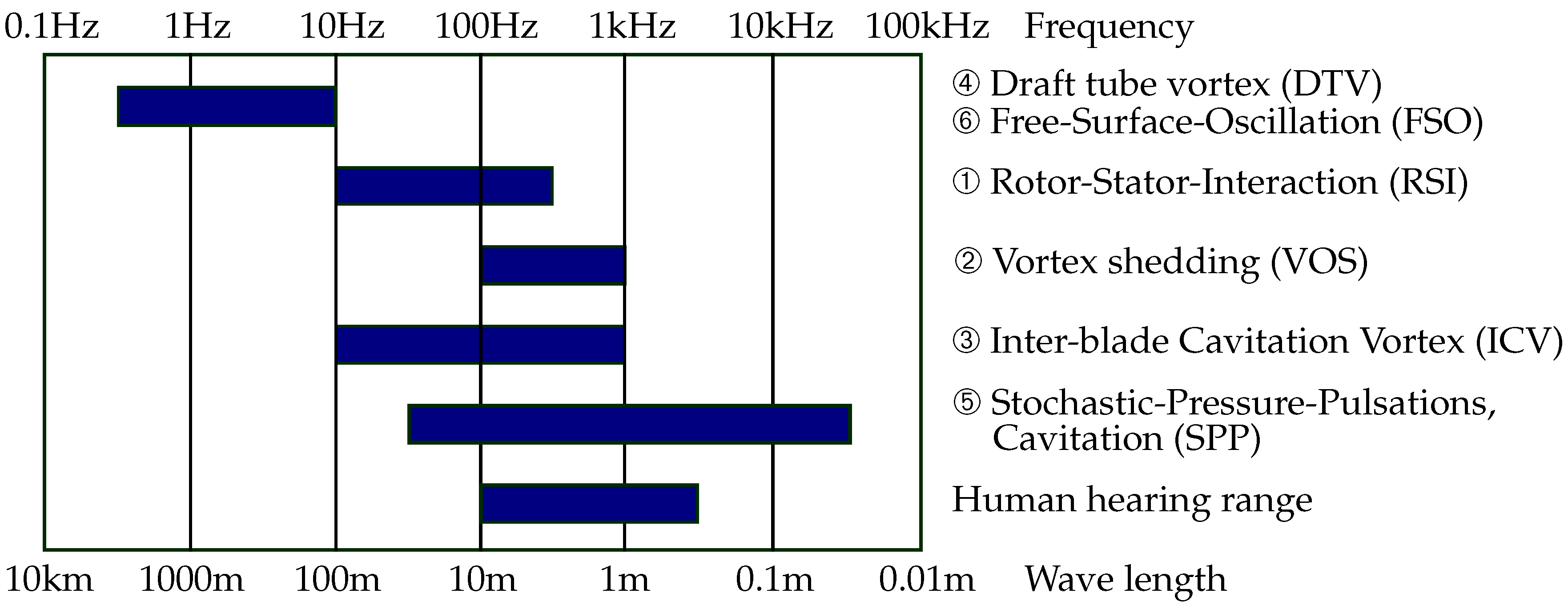
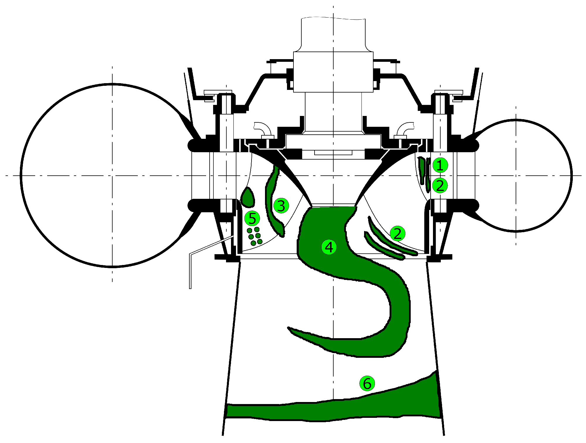
2.2. Flow Phenomena
2.3. Frequencies of Flow Phenomena
2.4. Damage Regions
3. State-of-the-Art in Lifetime Assessment
3.1. Numerical Tools and Measurement Techniques
3.1.1. Steady/Unsteady CFD Simulations
- (1)
- Time-averaged for the static FE analysis; however, in this case, only load steps with constant speed (synchronisation speed) can be calculated (see Section 3.1.3).
- (2)
- Fourier transformed and split-up in amplitude and phase parts, to be used for subsequent HRA investigations (see Section 3.3.2).
- (3)
- used directly as a time signal for a transient FEM (see Section 4.2.2).
3.1.2. Fluid–Structure Interaction (FSI)
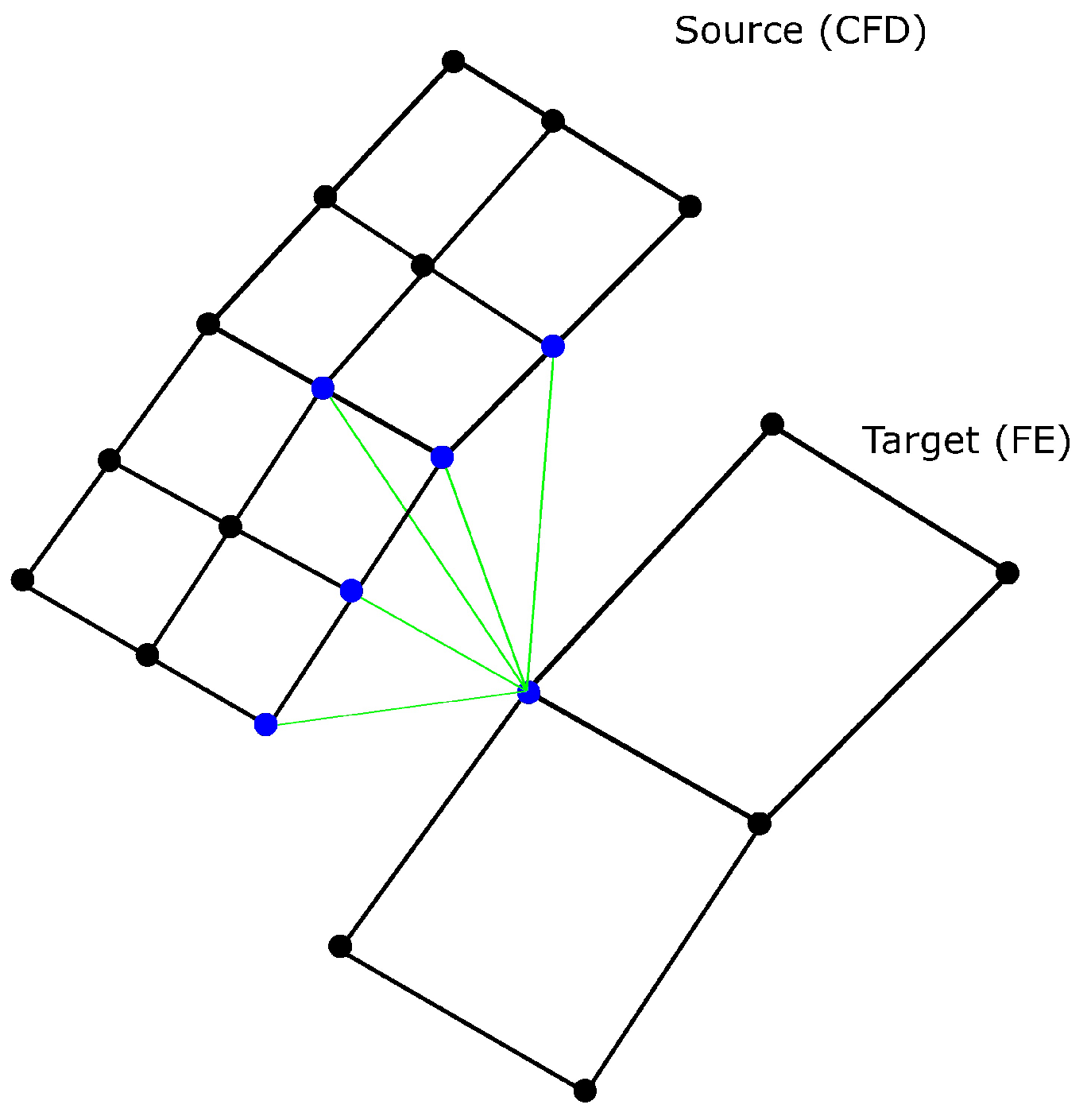
- Next-Neighbor Interpolation (Distance-Based Average)This interpolation calculates the distance from one target-node to a specified number of source-nodes (five nodes in Figure 10). Those Distances are used to calculate weightings. Finally, the values of the source-nodes are proportionally added up for the value of the target-node. If only one source-node is used, then the so-called nearest-neighbor Interpolation is obtained.
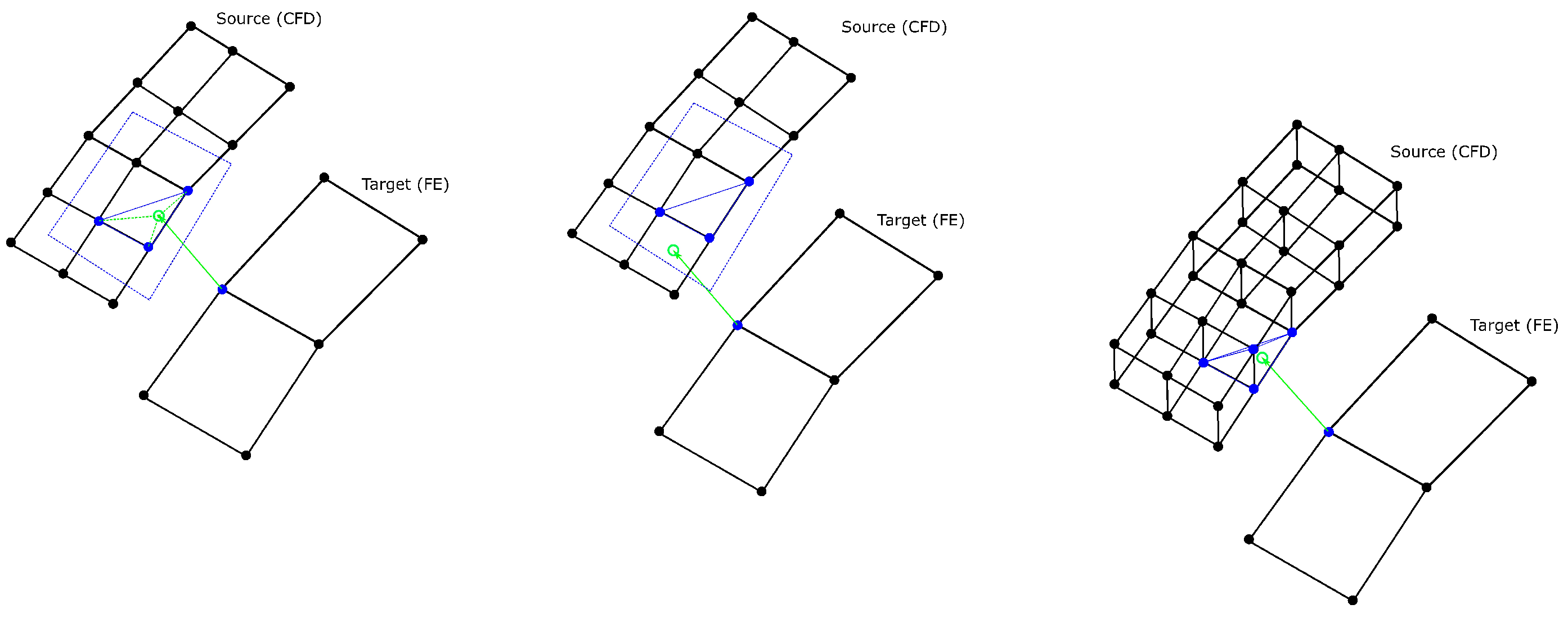
- TriangulationThe algorithm creates temporary elements with source-nodes in which the target-node is projected. Those elements are of two types:
- Surface: the target-node is projected onto a plane of a triangle (three source-points used)
- Volumetric: the target-node is projected into a tetrahedron (four source-points used)
For the creation of the elements, the nearest source-nodes are preferred. If the projected target-point is located outside of the created element (Figure 11), the next nodes are considered. The number of considered nodes is limited by a certain number (default is 20). In case that every projection is located outside the elements, the distance-based average method is used instead.
3.1.3. Static FEM Simulations
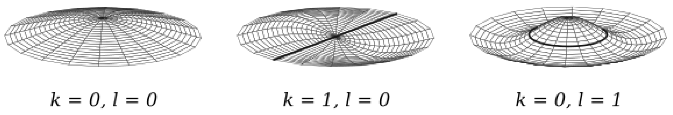
3.1.4. Modal Analysis (Natural Frequencies)
3.1.5. Harmonic Response Analysis
3.1.6. Measurement Techniques
3.2. Damage Hypotheses
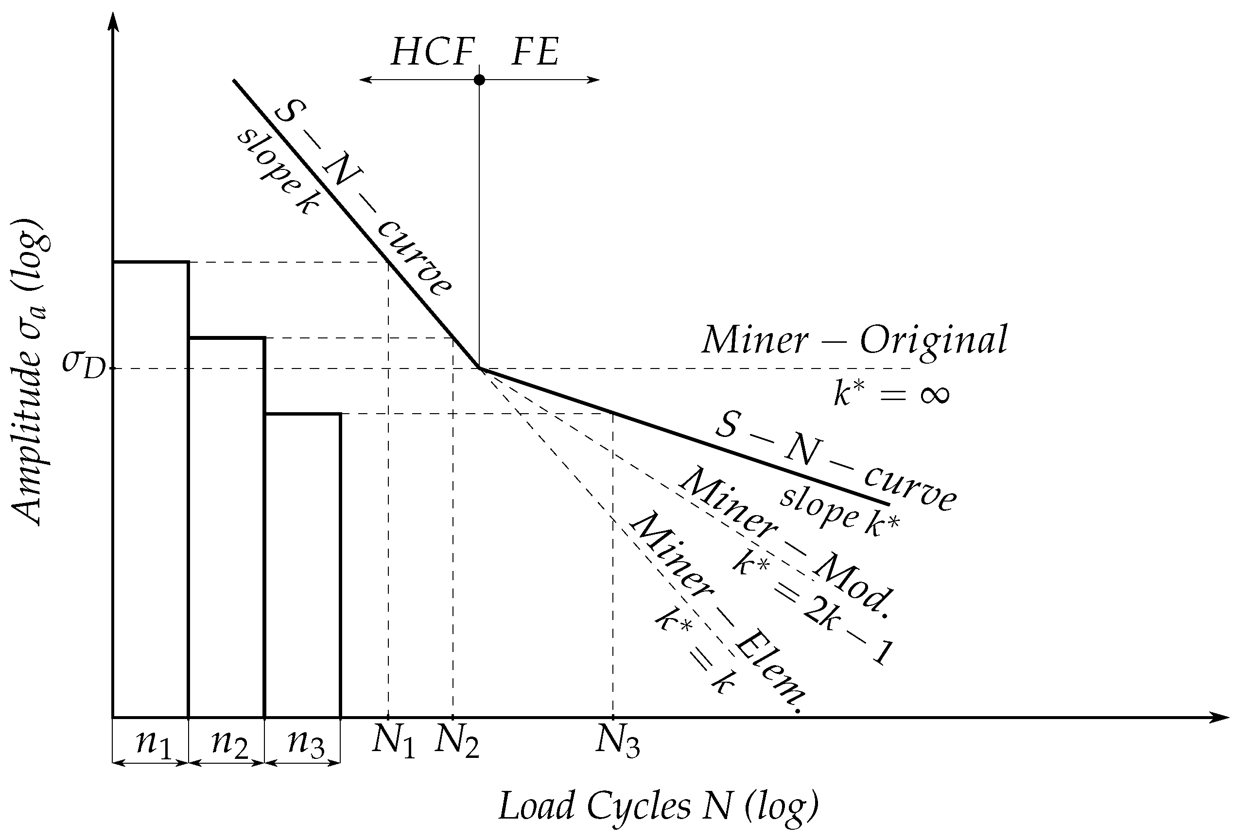
3.2.1. Palmgren–Miner on Fatigue Calculation before Crack
3.2.2. Fracture Mechanics of Crack Propagation
3.3. Lifetime Prediction
3.3.1. Stress Concentration Factor (k-Factor Concept) and Lifetime Assessment
3.3.2. HRA, Damage Factors and Lifetime Assessment
3.4. Summary
- (1)
- The state-of-the-art procedure is a fast method to determine the required data considering lower computer capacity.
- (2)
- Although this state-of-the-art method is not sufficient, it cannot be omitted because the mean stress and stress amplitude are needed for fatigue strength determinations.
- (3)
- The HRA can close the gap between static and dynamic approach but only for one precise frequency. One special flow phenomena with one particular frequency can be observed. For this excitation frequency the remaining lifetime can be calculated. HRA is in the middle between static investigation and totally unsteady/transient simulations. The advantage is the lower simulation time and faster approach.
- (4)
- Since this method can only represent load shifts with a synchronized machine, the simulation of transient operating conditions (STU, CMO, LR) are not possible.
- (5)
- In this case, the permanent machine diagnosis is seen more as a monitoring tool and less suitable for determining the lifetime.
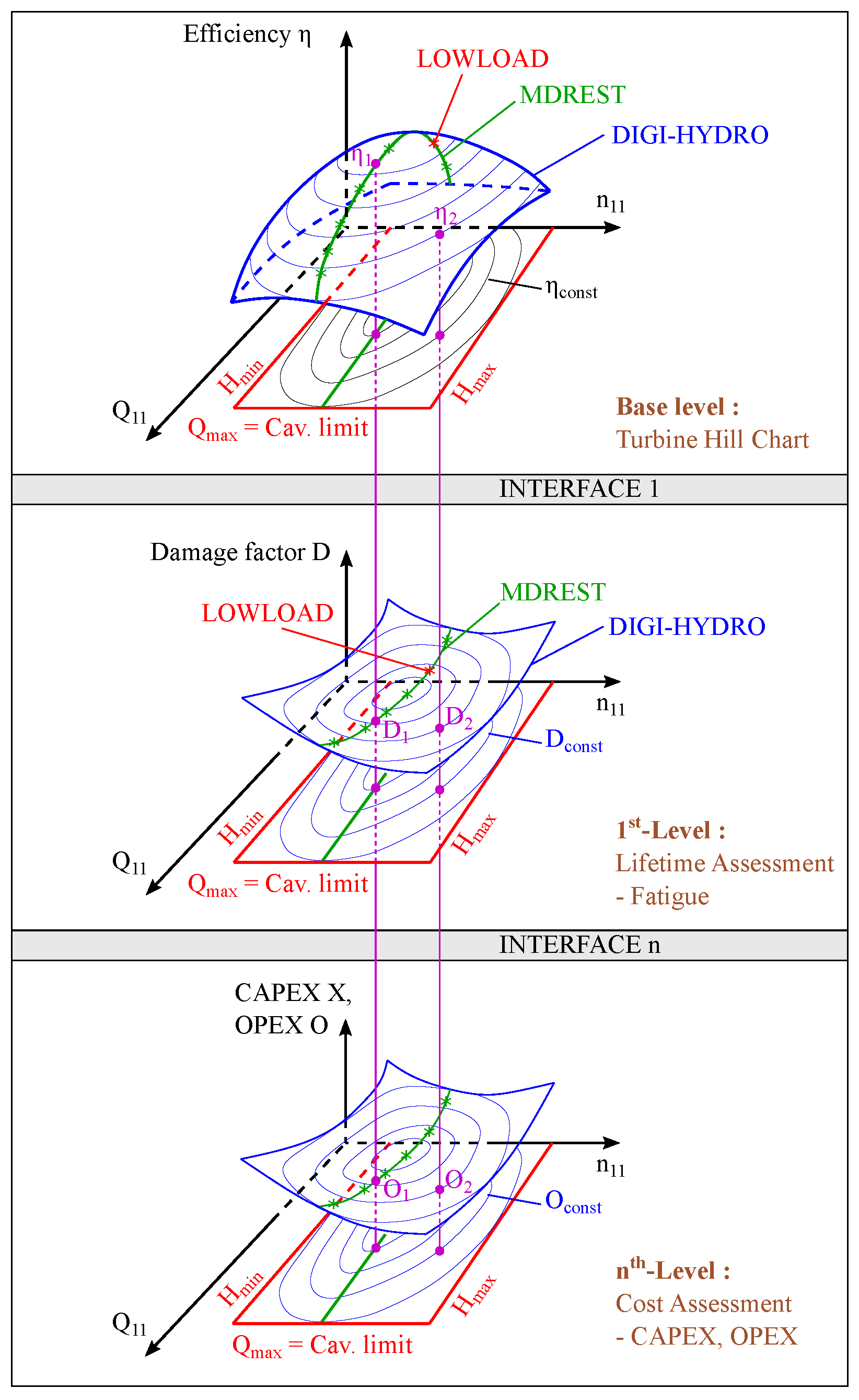
4. Multilevel Approach
- (1)
- Due to the increased part-load operation of the machine set, a static stress analysis is no longer permissible.
- (2)
- In the method development, it is necessary to distinguish whether one is still in the elastic stress range or already in the plastic one. Assuming that at least one crack is already present, fracture mechanics methods have to be applied. Otherwise, the fatigue analysis can suffice.
- (3)
- All load steps must be included in consideration of the damage—the more refined the gradation, the more accurate the method.
- (4)
- Attention must be paid to the validation of the numerically calculated results. Numerical methods contain many sources of error that must be handled with care.
- (5)
- The lifetime calculation is based on real measurements, on the one hand, and certain assumptions on the other hand. The result of such a lifetime assessment should therefore be seen as an indicator and critically reviewed.
- (6)
- When developing such an assessment tool, a mix of real prototype measurements and numerical calculations will be the most cost-effective option. Most of the time, the stress hotspot is unknown in the prototype measurement or a sensor application is not possible there. Only the combination brings this option of component assessment.
4.1. General Overview
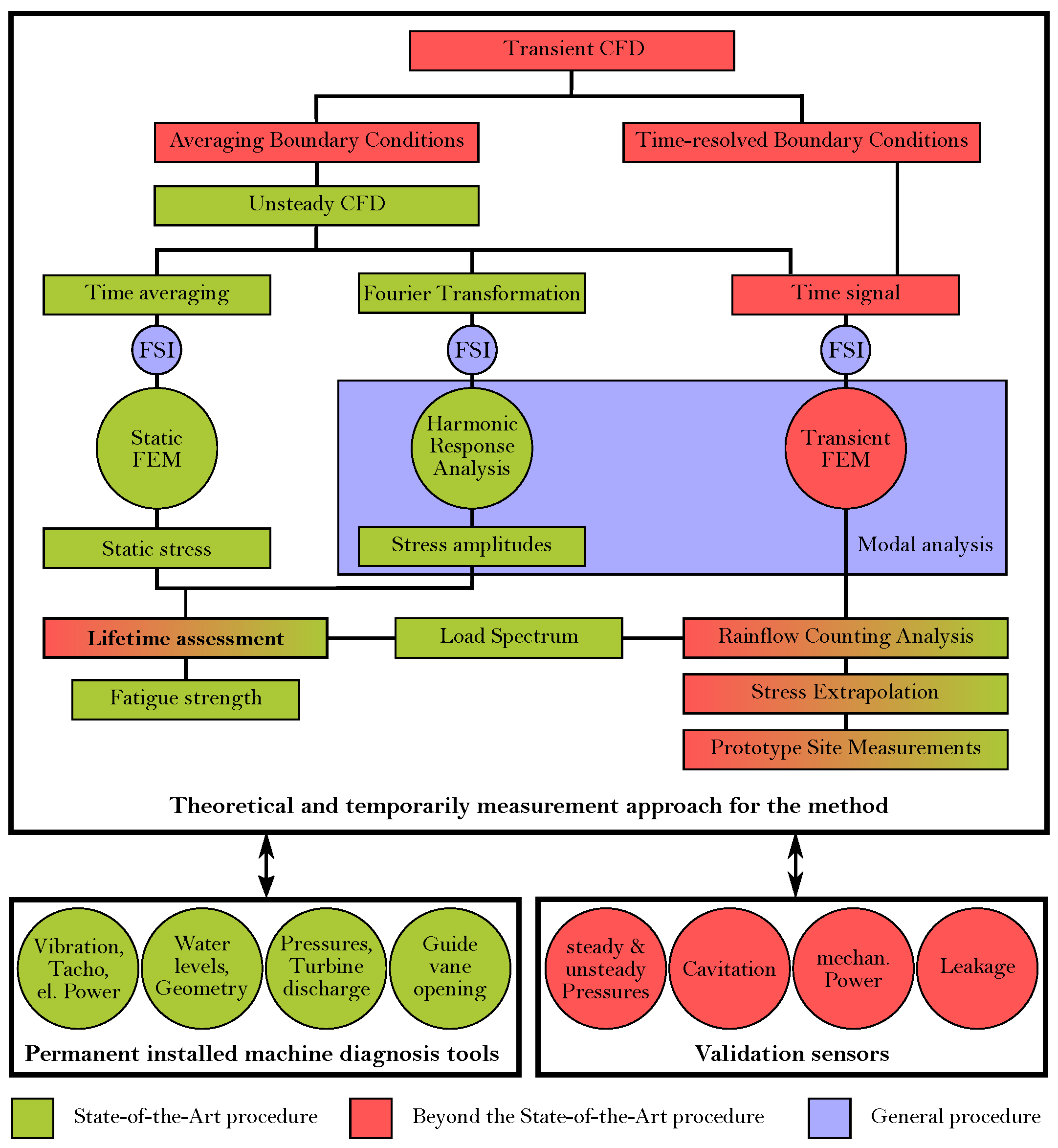
4.2. Beyond the State-of-the-Art Investigations—The Transient Assessment Model
4.2.1. Transient CFD Simulations
4.2.2. Transient FE Simulations
4.2.3. Damage Factors and Lifetime Prediction
4.2.4. Validation Measurements
5. Results
6. Conclusions/Outlook
- (1)
- Part I—model development and general overview
- (2)
- Part II—application and numerical lifetime calculation
- (3)
- Part III—measurements and lifetime investigation
- (4)
- Part IV–failure investigation, uncertainties, validation of lifetime calculation
Author Contributions
Funding
Institutional Review Board Statement
Informed Consent Statement
Data Availability Statement
Acknowledgments
Conflicts of Interest
Abbreviations
| a | crack length | (m) |
| BC | boundary conditions | |
| BP | best point | |
| structural damping matrix | (kg/s) | |
| CFD | computational fluid dynamics | |
| CMO | condenser mode | |
| CSM | computational structural mechanics | |
| characteristic length | (m) | |
| characteristic length factor | (m) | |
| d | trailing-edge thickness | (m) |
| partial damages | (-) | |
| D | damage factor | (-) |
| DTV | draft-tube vortex | |
| DSO | distribution system operator | |
| ENTSO-E | European Network of Transmission System Operators | |
| load vector | (N) | |
| FEM | finite element | |
| rotating frequency of the machine unit | (Hz) | |
| draft-tube vortex precession frequency | (Hz) | |
| draft-tube vortex pressure field frequency | (Hz) | |
| gate-passing frequency | (Hz) | |
| vortex-shedding frequency | (Hz) | |
| FSI | fluid–structure interaction | |
| FSO | free-surface oscillation | |
| GV | guide vane | |
| H | head at the turbine | (m) |
| head at the turbine at the rated point | (m) | |
| HPC | high-performance computing | |
| ICV | interblade cavitation vortex | |
| IoT | internet of things | |
| k | stress concentration factors | (-) |
| diametrical node number | (-) | |
| stress intensity factor | (-) | |
| structural stiffness matrix | (N/m) | |
| KPI | key performance indicators | |
| LL | low-load | |
| LR | load rejection | |
| harmonic order of the number of runner blades | (-) | |
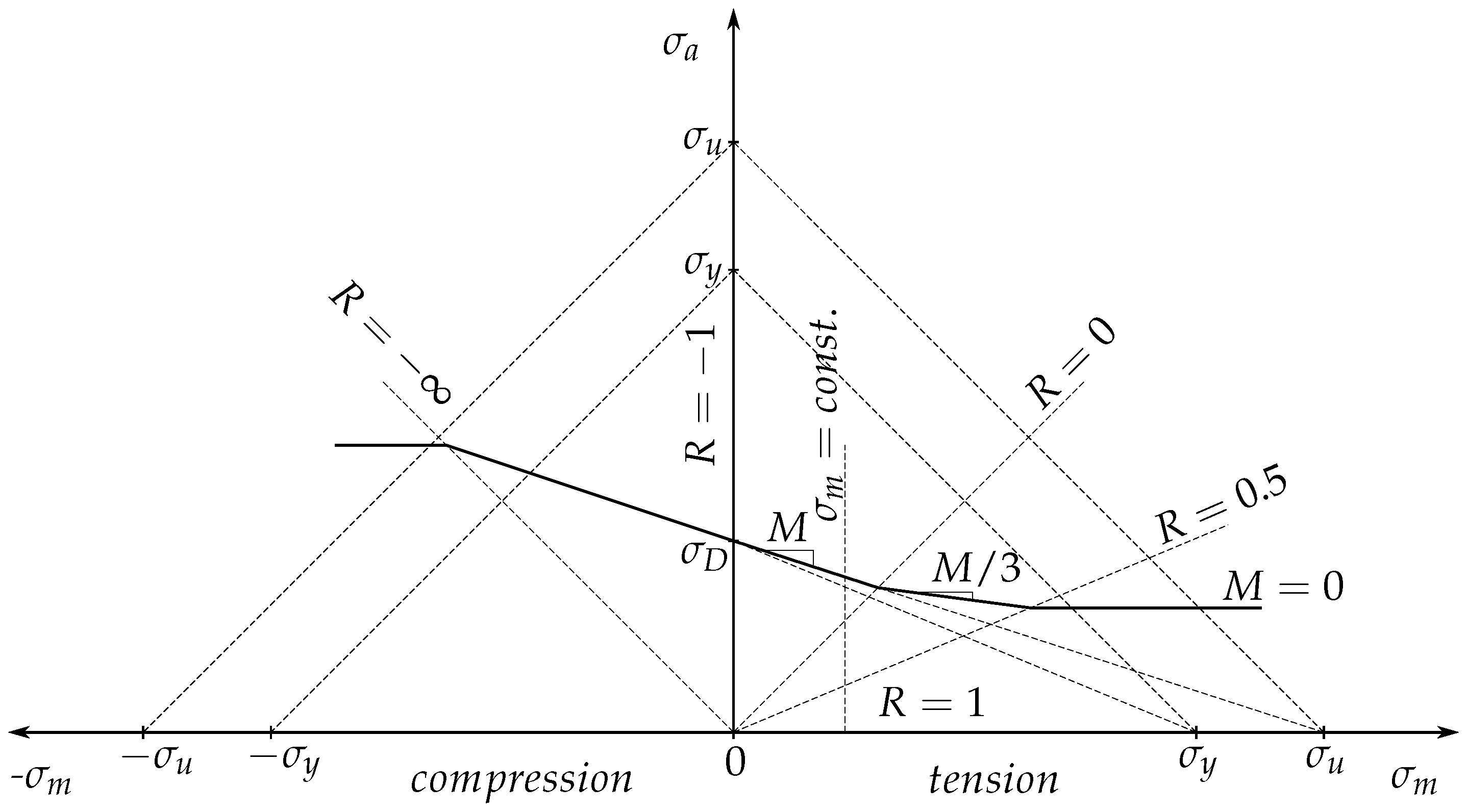
| M | mean stress sensitivity | (min) |
| structural mass matrix | (kg) | |
| kinematic viscosity | (m/s) | |
| n | turbine speed | (min) |
| harmonic order of the number of guide vanes | (-) | |
| speed factor according to IEC definition | (-) | |
| number of load cycles at amplitude | ||
| tolerable load cycles | ||
| specific speed | (min) | |
| NC | nodal circles | |
| ND | nodal diameters | |
| O and M | operation and maintenance | |
| P | power output | (W) |
| PL | part-load | - |
| Maximum Power Output of the Unit | (W) | |
| Power Output at Rated Point | (W) | |
| Q | Discharge at the turbine | [m/s] |
| Discharge factor according to IEC definition | (-) | |
| Discharge at the turbine at the rated point | (m/s) | |
| Dimensionless discharge coefficient | (-) | |
| Dimensionless discharge coefficient at best efficiency point | (-) | |
| R | Stress ratio | (-) |
| RANS | Reynolds averaged Navier-Stokes equations | |
| RFC | Rainflow Cylce Count | |
| RN | Runner | |
| RSI | Rotor-Stator-Interaction | |
| Dynamic stress (amplitude stress) | (N/mm) | |
| Vibration amplitude at category i | (N/mm) | |
| Mean stress | (N/mm) | |
| Stress cycle range | (N/mm) | |
| SHD | Shut-Down | |
| SNL | Speed-No-Load | |
| SPP | Stochastic-Pressure-Pulsations | |
| Strouhal number | (-) | |
| STU | Start-Up | |
| TSO | Transmission System Operator | |
| Nodal displacement vector | (m) | |
| URANS | Unsteady RANS | |
| V | Velocity of approach | (m/s) |
| Velocity of approach in x-direction | (m/s) | |
| VOS | Vortex Shedding | |
| x | Blade length | (m) |
| Stress intensity correction factor | (-) | |
| Number of guide vanes | (-) | |
| Number of runner blades | (-) |
References
- IG Windkraft. Installed Wind Power in Austria. Available online: https://www.igwindkraft.at/?xmlval_ID_KEY[0]=1029 (accessed on 16 November 2021).
- Bundesverband Photovoltaic Austria. Installed PV Power in Austria. Available online: https://pvaustria.at/daten-fakten/ (accessed on 16 November 2021).
- Energy Charts. Available online: https://energy-charts.info/index.html?l=en&c=DE (accessed on 16 November 2021).
- IEA. Hydropower Special Market Report: Analysis and Forecast to 2030; IEA: Paris, France, 2021. [Google Scholar]
- Inage, S.I. The role of large-scale energy storage under high shares of renewable energy. Wiley Interdiscip. Rev. Energy Environ. 2015, 4, 115–132. [Google Scholar] [CrossRef]
- Ahrens, R. Energiespeicher: Die Achillesferse des Smart Grid. Available online: https://www.ingenieur.de/technik/fachbereiche/energie/energiespeicher-achillesferse-smart-grid/ (accessed on 16 November 2021).
- BDEW. Erneuerbare Energien und das EEG: Zahlen, Fakten, Grafiken: Anlagen, installierte Leistung, Stromerzeugung, EEG-Vergütungssummen, Marktintegration der erneuerbaren Energien und regionale Verteilung der EEG-induzierten Zahlungsströme; BDEW Bundesverband der Energie- und Wasserwirtschaft e.V.: Berlin, Germany, 15 December 2011. [Google Scholar]
- DENA. Analyse der Notwendigkeit des Ausbaus von Pumpspeicherwerken und Anderen Stromspeichern zur Integration der Erneuerbaren Energien; Deutsche Energie Agentur (dena) GmbH: Berlin, Germany, 5 February 2010. [Google Scholar]
- DENA. Integration of Renewable Energy Sources in the German Power Supply System from 2015–2020 with an Outlook to 2025: Dena Grid Study II; Deutsche Energie Agentur (dena) GmbH: Berlin, Germany, April 2011. [Google Scholar]
- EURELECTRIC. Flexible Generation: Backing up Renewables; Union of the Electricity Industry—EURELECTRIC: Brussels, Belgium, October 2011. [Google Scholar]
- Moser, A.; Rotering, N.; Schäfer, A. Unterstützung der Energiewende in Deutschland Durch einen Pumpspeicherausbau: Potentiale zur Verbesserung der Wirtschaftlichkeit und der Versorgungssicherheit; Institut für Elektrische Anlagen und Energiewirtschaft: Aachen, Germany, April 2014. [Google Scholar]
- Leonard, W.; Buenger, U.; Crotogino, F.; Gatzen, C.H.; Glaunsinger, W.; Huebner, S.; Kleimeier, M.; Koenemund, M.; Landinger, H.; Lebioda, T.; et al. Energy Storage in Power Supply Systems with a High Share of Renewable Energy Sources: Significance, State of the Art, Need for Action; VDE Association for Electrical, Electronic Information Technologies: Frankfurt am Main/Berlin, Germany; Brussel, Belgium, 2008. [Google Scholar]
- Ibrahim, H.; Ilinca, A.; Perron, J. Energy storage systems—Characteristics and comparisons. Renew. Sustain. Energy Rev. 2008, 12, 1221–1250. [Google Scholar] [CrossRef]
- IEA; International Energy Agency. TECHNOLOGY ROADMAP: Energy Storage. In Springer Reference; Springer: Berlin/Heidelberg, Germany, 2011. [Google Scholar]
- HEA. Hydro Equipment Technology Roadmap; Hydro Equipment Association: Brussels, Belgium, August 2013. [Google Scholar]
- Lund, H.; Andersen, A.N.; Østergaard, P.A.; Mathiesen, B.V.; Connolly, D. From electricity smart grids to smart energy systems—A market operation based approach and understanding. Energy 2012, 42, 96–102. [Google Scholar] [CrossRef]
- Martini, L.; Brunner, H.; Rodriguez, E.; Caerts, C.; Strasser, T.I.; Burt, G.M. Grid of the future and the need for a decentralised control architecture: The web-of-cells concept. CIRED-Open Access Proc. J. 2017, 2017, 1162–1166. [Google Scholar] [CrossRef] [Green Version]
- IEA. Digitalization & Energy; International Energy Agency (IEA): Paris, France, 2017. [Google Scholar] [CrossRef]
- Hartnett, S.; Bronski, P. How Blockchain Can Manage the Future Electricity Grid. Available online: https://www.weforum.org/agenda/2018/05/how-blockchain-can-manage-the-electricity-grid/ (accessed on 16 November 2021).
- Greunsven, J.; Moser, A. TenneT Market Review 2017–Electricity Market Insights; TenneT Holding B.V. and TenneT TSO B.V.: Arnhem, The Netherlands, March 2018. [Google Scholar]
- Doujak, E. Effects of Increased Solar and Wind Energy on Hydro Plant Operation. HRW 2014, 22, 28–31. [Google Scholar]
- Sick, M.; Michler, W.; Winkler, S.; Wurm, E.; Désy, N.; Coutu, A. Flexible turbine operation enabling frequency control. In Proceedings of the HYDRO 2012, Bilbao, Portugal, 29–31 October 2012. [Google Scholar]
- Sick, M.; Oram, C.; Braun, O.; Nennemann, B.; Coutu, A. Hydro projects delivering regulating power: Technical challenges and cost of operation. In Proceedings of the HYDRO 2013, Innsbruck, Austria, 7–9 October 2013. [Google Scholar]
- Unterluggauer, J.; Doujak, E.; Bauer, C. Fatigue analysis of a prototype Francis turbine based on strain gauge measurements. WasserWirtschaft Extra 2019, 109, 66–71. [Google Scholar] [CrossRef]
- BDEW. Die digitale Energiewirtschaft: Agenda für Unternehmen und Politik; BDEW Bundesverband der Energie- und Wasserwirtschaft e.V.: Berlin, Germany, 2015. [Google Scholar]
- Coutu, A.; Aunemo, H.; Badding, B.; Velagandula, O. Dynamic behaviour of high head Francis turbines. In Proceedings of the HYDRO 2005, Villach, Austria, 17–21 October 2005; pp. 1–7. [Google Scholar]
- Coutu, A.; Monette, C.; Velagandula, O. Francis Runner Dynamic Stress Calculations. In Proceedings of the HYDRO 2007, Grenada, Spain, 15–18 October 2007. [Google Scholar]
- Egusquiza, E.; Valero, C.; Huang, X.; Jou, E.; Guardo, A.; Rodriguez, C. Failure investigation of a large pump-turbine runner. Eng. Fail. Anal. 2012, 23, 27–34. [Google Scholar] [CrossRef] [Green Version]
- Magnoli, M.V. Numerical simulation of pressure oscillations in large Francis turbines at partial and full load operating conditions and their effects on the runner structural behaviour and fatigue life. Ph.D. Thesis, Technische Universität München, München, Germany, 2015. [Google Scholar]
- Coutu, A.; Chamberland-Lauzon, J. The impact of flexible operation on Francis runners. Int. J. Hydropower Dams 2015, 22, 90–93. [Google Scholar]
- Doujak, E.; Eichhorn, M. An Approach to Evaluate the Lifetime of a High Head Francis runner. In Proceedings of the 16th International Symposium on Transport Phenomena and Dynamics of Rotating Machinery, Honolulu, HI, USA, 10–15 April 2016. [Google Scholar]
- Eichhorn, M.; Doujak, E. Impact of Different Operating Conditions on the Dynamic Excitation of a High Head Francis Turbine. In Proceedings of the ASME 2016 International Mechanical Engineering Congress & Exposition (IMECE 2016), Phoenix, AZ, USA,, 11–17 November 2016; p. V04AT05A035. [Google Scholar] [CrossRef]
- Duparchy, F.; Brammer, J.; Thibaud, M.; Favrel, A.; Lowys, P.Y.; Avellan, F. Mechanical impact of dynamic phenomena in Francis turbines at off design conditions. J. Phys. Conf. Ser. 2017, 813, 012035. [Google Scholar] [CrossRef] [Green Version]
- Escaler, X.; Egusquiza, E.; Farhat, M.; Avellan, F.; Coussirat, M. Detection of cavitation in hydraulic turbines. Mech. Syst. Signal Process. 2006, 20, 983–1007. [Google Scholar] [CrossRef] [Green Version]
- Dörfler, P.; Sick, M.; Coutu, A. Flow-Induced Pulsation and Vibration in Hydroelectric Machinery: Engineer’s Guidebook for Planning, Design and Troubleshooting; Springer: London, UK; New York, NY, USA, 2013. [Google Scholar]
- Seidel, U.; Hübner, B.; Löfflad, J.; Faigle, P. Evaluation of RSI-induced stresses in Francis runners. In Proceedings of the 26th IAHR Symposium on Hydraulic Machinery and Systems, Beijing, China, 19–23 August 2012; Volume 15, p. 52010. [Google Scholar] [CrossRef]
- Trivedi, C.; Gandhi, B.; Cervantes, M.J. Effect of transients on Francis turbine runner life: A review. J. Hydraul. Res. 2013, 51, 121–132. [Google Scholar] [CrossRef]
- Liu, X.; Luo, Y.; Wang, Z. A review on fatigue damage mechanism in hydro turbines. Renew. Sustain. Energy Rev. 2016, 54, 1–14. [Google Scholar] [CrossRef]
- De Boer, A.; Van Zuijlen, A.H.; Bijl, H. Comparison of the conservative and a consistent approach for the coupling of non-matching meshes. In Proceedings/European Conference on Computational Fluid Dynamics; Wesseling, P., Ed.; TU: Delft, The Netherlands, 2006. [Google Scholar]
- Doujak, E.; Unterluggauer, J. Fluid-structure interaction of Francis turbines at different load steps. In Proceedings of the 9th International Symposium on Fluid-Structure Interactions, Flow-Sound Interactions, Flow-Induced Vibration & Noise, Toronto, Kanada, 8–11 July 2018. [Google Scholar]
- Flores, M.; Urquiza, G.; Rodríguez, J.M. A Fatigue Analysis of a Hydraulic Francis Turbine Runner. World J. Mech. 2012, 2, 28–34. [Google Scholar] [CrossRef] [Green Version]
- Guillaume, R.; Deniau, J.L.; Scolaro, D.; Colombet, C. Influence of rotor-stator interaction on the dynamic stresses of Francis runners. In Proceedings of the 26th IAHR Symposium on Hydraulic Machinery and Systems, Beijing, China, 19–23 August 2012; Volume 15, p. 52011. [Google Scholar] [CrossRef]
- Wauer, J. Kontinuumsschwingungen: Vom Einfachen Strukturmodell zum Komplexen Mehrfeldsystem; GWV Fachverlage GmbH: Wiesbaden, Germany, 2008. [Google Scholar] [CrossRef]
- Palmgren, A. Die Lebensdauer von Kugellagern. VDI Zeitschrift 1924, 68, 339–341. [Google Scholar]
- Miner, M.A. Cumulative Damage in Fatigue. J. Appl. Mech. 1945, 12, 159–164. [Google Scholar] [CrossRef]
- Köhler, M.; Jenne, S.; Pötter, K.; Zenner, H. Zählverfahren und Lastannahme in der Betriebsfestigkeit; Springer: Berlin/Heidelberg, Germany, 2012. [Google Scholar] [CrossRef]
- Johannesson, P. Extrapolation of load histories and spectra. Fatigue Fract. Eng. Mater. Struct. 2006, 29, 209–217. [Google Scholar] [CrossRef] [Green Version]
- Haibach, E. Betriebsfestigkeit, 3rd ed.; Springer: Berlin/Heidelberg, Germany, 2006. [Google Scholar]
- Radaj, D.; Vormwald, M. Ermüdungsfestigkeit, 3rd ed.; Springer: Berlin/Heidelberg, Germany, 2007. [Google Scholar]
- Byrne, J. Influence of LCF overloads on combined HCF/LCF crack growth. Int. J. Fatigue 2003, 25, 827–834. [Google Scholar] [CrossRef]
- Ciavarella, M.; Monno, F. On the possible generalizations of the Kitagawa–Takahashi diagram and of the El Haddad equation to finite life. Int. J. Fatigue 2006, 28, 1826–1837. [Google Scholar] [CrossRef]
- Ditlevsen, O.; Madsen, H.O. Structural Reliability Methods: 2.3.7 web ed.; Technical University of Denmark: Lyngby, Denmark, 2007. [Google Scholar]
- Gagnon, M.; Tahan, S.A.; Bocher, P.; Thibault, D. The role of high cycle fatigue (HCF) onset in Francis runner reliability. IOP Conf. Ser. Earth Environ. Sci. 2012, 15, 22005. [Google Scholar] [CrossRef] [Green Version]
- Gagnon, M.; Tahan, A.; Bocher, P.; Thibault, D. On the stochastic simulation of hydroelectric turbine blades transient response. Mech. Syst. Signal Process. 2012, 32, 178–187. [Google Scholar] [CrossRef]
- Gagnon, M.; Tahan, A.; Bocher, P.; Thibault, D. A probabilistic model for the onset of High Cycle Fatigue (HCF) crack propagation: Application to hydroelectric turbine runner. Int. J. Fatigue 2013, 47, 300–307. [Google Scholar] [CrossRef]
- Diagne, I.; Gagnon, M.; Tahan, A. Modeling the dynamic behavior of turbine runner blades during transients using indirect measurements. In Proceedings of the 28th IAHR Symposium on Hydraulic Machinery and Systems, Grenoble, France, 4–8 July 2016. [Google Scholar] [CrossRef] [Green Version]
- Pollak, R.D. Analysis of Methods for Determining High Cycle Fatigue Strength of a Material with Investigation of Ti-6al-4v Gigacycle Fatigue Behavior. Ph.D. Thesis, Air University, Wright-Patterson Air Force Base, OH, USA, 2005. [Google Scholar]
- Matsumoto, Y.; Okude, K.; Aoyama, J.; Iida, I.; Funato, K.; Hiramatsu, Y. Development of new remaining life estimation method for main parts of hydroturbine in hydroelectric power plant. In Proceedings of the 23rd IAHR Symposium on Hydraulic Machinery and Systems, Yokohama, Japan, 17–21 October 2006. [Google Scholar]
- Unterluggauer, J.; Doujak, E.; Bauer, C. Fatigue analysis of a prototype Francis Turbine based on strain gauge measurements. In 20. Internationales Seminar Wasserkraftanlagen //20th International Seminar on Hydropower Plants; Technische Universität Wien, Ed.; Eigenverlag: Wien, Austria, 2018; pp. 707–720. [Google Scholar]
- Eichhorn, M.; Taruffi, A.; Bauer, C. Expected load spectra of prototype Francis turbines in low-load operation using numerical simulations and site measurements. J. Phys. Conf. Ser. 2017, 813, 012052. [Google Scholar] [CrossRef] [Green Version]


| Type of Control Energy | FCR | aFRR | mFRR |
|---|---|---|---|
| Provided by | ENTSO-E | TSO | TSO |
| activation | frequency-controlled; independent measurement/intervention on site by FCR provider | by control area responsible TSO-automatically replaces FCR | by control area responsible TSO-manual request by TSO |
| full power | within 30 s | within 5 min | within 15 min |
| period to be covered after an incident | 0–15 min | from 30 s to 15 min | from 15 min to 60 min |
| remuneration | demand rate | demand and energy rate | demand and energy rate |
| minimum bid size | From +/− 1 MW (symmetrical) | 5 MW positive or negative | 5 MW positive or negative |
| daily products | positive and negative: 6 time slices over 4 h | positive and negative: 6 time slices over 4 h | positive and negative: 6 time slices over 4 h |
| Operational Region | Deterministic | Stochastic |
|---|---|---|
| start-up (STU) | RSI, VOS | SPP, VOS |
| speed–no-load (SNL) | RSI, VOS | SPP, VOS |
| low-load (LL) | RSI, (VOS, DTV) | ICV, SPP, VOS |
| part-load (PL) | RSI, DTV | (ICV, SPP), VOS |
| best point (BP) | RSI | |
| full-load (FL) | RSI, DTV | |
| condenser mode (CMO) | FSO | (DTV) |
| Method | Mean Stress | RSI | VOS | ICV | DTV | SPP | FSO |
|---|---|---|---|---|---|---|---|
| k-factor concept (Section 3.3.1) | yes | no | no | no | no | no | no |
| HRA (Section 3.3.2) | yes | yes | yes | no | yes | no | no |
| transient assessment (Section 4.2.3) | yes | yes | yes | yes | yes | yes | yes |
| Position | Base Load | Grid Stabilization |
|---|---|---|
| [Years] | [Years] | |
| computed HS1 | 13,517 | 363 |
| validated HS1 | 83 | |
| computed HS2 | 22,676 | 47 |
| validated HS2 | 761 |
Publisher’s Note: MDPI stays neutral with regard to jurisdictional claims in published maps and institutional affiliations. |
© 2022 by the authors. Licensee MDPI, Basel, Switzerland. This article is an open access article distributed under the terms and conditions of the Creative Commons Attribution (CC BY) license (https://creativecommons.org/licenses/by/4.0/).
Share and Cite
Doujak, E.; Stadler, S.; Fillinger, G.; Haller, F.; Maier, M.; Nocker, A.; Gaßner, J.; Unterluggauer, J. Fatigue Strength Analysis of a Prototype Francis Turbine in a Multilevel Lifetime Assessment Procedure Part I: Background, Theory and Assessment Procedure Development. Energies 2022, 15, 1148. https://doi.org/10.3390/en15031148
Doujak E, Stadler S, Fillinger G, Haller F, Maier M, Nocker A, Gaßner J, Unterluggauer J. Fatigue Strength Analysis of a Prototype Francis Turbine in a Multilevel Lifetime Assessment Procedure Part I: Background, Theory and Assessment Procedure Development. Energies. 2022; 15(3):1148. https://doi.org/10.3390/en15031148
Chicago/Turabian StyleDoujak, Eduard, Simon Stadler, Gerald Fillinger, Franz Haller, Michael Maier, Armin Nocker, Johannes Gaßner, and Julian Unterluggauer. 2022. "Fatigue Strength Analysis of a Prototype Francis Turbine in a Multilevel Lifetime Assessment Procedure Part I: Background, Theory and Assessment Procedure Development" Energies 15, no. 3: 1148. https://doi.org/10.3390/en15031148
APA StyleDoujak, E., Stadler, S., Fillinger, G., Haller, F., Maier, M., Nocker, A., Gaßner, J., & Unterluggauer, J. (2022). Fatigue Strength Analysis of a Prototype Francis Turbine in a Multilevel Lifetime Assessment Procedure Part I: Background, Theory and Assessment Procedure Development. Energies, 15(3), 1148. https://doi.org/10.3390/en15031148