Fatigue Strength Analysis of a Prototype Francis Turbine in a Multilevel Lifetime Assessment Procedure Part II: Method Application and Numerical Investigation

Abstract

Part I of the publication series addressed the fundamentals of lifetime assessment of prototype Francis turbines. This paper (Part II) focuses on the numerical part of the procedure. The essential steps and requirements shall be presented (background). The starting points for the numerical considerations are the pressure fields of the transient CFD simulations, which are exported per time step and applied to the existing structure via a fluid–structure interaction. That enables a transient mechanical stress calculation to be conducted, resulting in the fatigue analysis of the component to estimate the remaining lifetime. The individual model requirements should be represented accordingly and applied to the prototype facility (method). The results obtained from this application should be discussed and evaluated. It has to be mentioned that the validation of the numerical results will be performed at Part IV of this publication series (results). The present paper will end up discussing the results and conclusions about further data processing (Conclusion).

1. Introduction

Numerical simulation has become indispensable in the design of hydraulic turbines. However, the question of the effort required for the design and calculation of the components arises. PART I of the publication series already described the state-of-the-art in this field. The state of the art is the mean-stress concept or the calculation of individual exciting frequencies in the system. The system responses to these particular excitation frequencies are determined through Harmonic Response Analysis (HRA). However, as already shown at PART I of this publication series, more complex modelling and more elaborate computation is required to calculate the issues of transient operating conditions or flow phenomena in the deep part-load region. This part of the publication concentrates on the methods used, the boundary conditions applied and those parameters that have a decisive influence on the entire calculation area. We distinguish between fluid mechanics and solid mechanics. In order to be able to transfer the corresponding information from fluid mechanics to structural mechanics, suitable coupling algorithms are needed.

Researchers worldwide have already published a wide variety of singular observations of flow phenomena and interactions with structure. In this chapter, a brief outline of the most important publications in numerical simulation of the last four to five years will be given. According to Section 2.1 from PART I, the classification was chosen to structure the literature study. The rotor–stator interaction ➀ forms the beginning. This phenomenon, as described earlier, is only dependent on the number of vanes and blades. Publication [1], from 2012, raises the rotor-stator interaction impact on the runner’s dynamic loads. Publication [2], which already provides a review of the numerical methods at that time, dates from the same year. Emerging energy storage problems and the related investigation of pump-turbines are shown at [3], which deals with the rotor-stator interaction of a pump-turbine in turbine operation. Publication [4] shows the extent to which open source software is already being used. Here, OpenFoam was used for the numerical calculation of the rotor-stator interaction of Francis turbines. Publication [5] deals already with the investigation of guide vane as part of the rotor-stator interaction. It is no longer just the runner itself under investigation, but the guide vane in front of it is already included in the considerations.

The next phenomenon in the line is the vortex shedding ➁. That is the detachment of a flow behind a body or an edge. Inside a hydraulic turbine, there are always edges and vertices where the flow can detach and cause these well-known and distinctive vortex formations. As more sophisticated turbulence models for numerical calculation of this phenomenon are required, and more complex meshes are necessary, the number of relevant publications is relatively tiny. Mostly, it is experimental investigations that provide a basis for the validation, such as [6] of 2019, or singular analysis of individual components, see [7] in 2017, without investigating the effects on the entire unit.

An approximately similar situation is found at the interblade-vortex ➂ flow phenomenon. Again, the resources for numerical simulations are very high, and therefore only a few all-encompassing simulations have been published. Since interblade-vortex only occurs at low-load operation, the corresponding investigations are also from the recent past. Two representative publications, namely [8,9] from 2017, deal with this flow structure’s occurrence and characteristics in a Francis turbine. They show the flow effect based on numerical simulations. However, the mechanical effects on the structure are missing, as they are tough to validate.

There are considerably more publications on the draft tube vortex ➃. The overload domain is currently the most intensively researched operational area. Publications in this area deal with the unstable behavior of the flow phenomenon and its effects on the machine unit’s power output. This draft tube vortex’s high energy content and its transient behavior lead to undesired power swings, which are replicated in the electrical grid (see [10]). In the case of the part-load draft tube vortex, the question of origin is no longer an issue but rather the exact determination of the impacts. This flow phenomenon causes pressure fluctuations and transient vortex structures in the draft tube as well as fluctuations at the turbine shaft, which are responsible for power swings as oscillating torque. A basic understanding of the occurrence of the draft tube vortex is provided by [11], while [12] already uses two-phase cavitation models for the precise determination of the pressure fields. The influence of different blade lengths and water admission to avoid this effect are discussed in [13,14]. The dependence of the draft tube vortex on the tailwater level was investigated by [15]. The last three publications already attempt to present parameters for countermeasures.

The complexity of cavitation ➄ has prevented more precise numerical calculations and validations. Mainly the extremely high frequencies of this physical effect pose a challenge to the simulation. Therefore, hardly any more detailed investigations exist, which are also validated by a corresponding measurement. The appearance of cavitation as a local pressure drop below the vapor pressure tends to be evaluated globally and not at the level of individual bubbles. Experimental results in this field have been published, but numerical results have so far been limited to explaining the fundamentals. Occasionally, one sees publications that touch on this topic to investigate design countermeasures (see [16]). The stochastic pressure pulsations ➄ at deep part-load operating areas show a similar pattern. One recognizes a multitude of different frequencies. However, not all of them have been researched yet. Some of these amplitude peaks are natural frequencies, and others are excitation frequencies. Therefore, it is essential to develop a method that analyses and evaluates all frequencies in one system.

The free oscillating water surface’s ➅ research field during synchronous condenser mode of a Francis turbine is relatively new. This mode is used by the generator side to supply grid stabilization measures, such as phase regulation and reactive power delivery. In Austria, selected hydropower plants are equipped for this operational mode and support the electrical grid with their services. Here, the turbine is drained with compressed air and operated in air. The water is pressed into the draft tube cone and remains there until the turbine is refilled for regular operation. If this process lasts for a longer time, a rotating wave develops on the water surface. This phenomenon is called oscillating water surface or sloshing and was investigated (2017) by [17]. This air-water system’s excitation mechanism is still not proven from a fluid mechanics point of view. In 2019, reference [18] provides a theoretical background and [19] basic experimental investigations on a laboratory test rig.

All listed flow phenomena interact with the Francis turbine as a rigid body and have to be coupled with structural mechanic fatigue investigation. A review of fluid–structure interactions in Francis turbines was provided by [20]. Mapping methods manage the data transfer between CFD and FE meshes. They are necessary because each mesh is optimized for the respective application, and hence they are not congruent at the interface. The mapping methods’ influence on the systematic error during data transfer was investigated in [21].

In addition to the fatigue assessment, the modal analysis of a runner is of crucial importance. Knowing the natural frequency and eigenmode of a component is the only way to estimate how sensitive it is to fail in resonance conditions. Since the runner rotates in water, the surrounding water masses change the part’s natural frequency and eigenmodes. Issues of the oscillating water masses, stiffness and damping of the coupled system have to be considered. Added mass effects are known for a long time and have already been scientifically investigated. More attention has been paid to the damping and stiffness effects of the water in combination with the structure (see [22]). The complexity of this research relates to the validation of the mathematical contexts and the resulting numerical simulations. It is therefore essential that numerical results are properly validated (see, e.g., [23]). Including two-phase flows into the considerations results in complex investigations, as shown in [24], where added mass effects were combined with blade cavitation.

The number of new publications in fatigue analysis of Francis turbines in recent years shows the increased research activities. All publications focus on the deep part-load range, as the flow phenomena occurring in this operating range have a significant impact on the runner’s lifetime. However, taking a closer look at the research activities, different approaches are recognisable: Reference [25] deals with the necessary turbulence modelling to create a balance between simulation time and result accuracy. The BSL-EARSM turbulence model at load step $(Q/Q_{BEP}=0.27)$ has been applied. Reference [26] investigated the deep part-load range of a model pump-turbine in pumping mode. Reference [27] investigated this range in turbine mode. References [6,28,29,30] performed their investigations on prototype plants and thus excluding scaling effects from model to prototype.

This short literature review shows that there is still room for further development and research work, especially in terms of a holistic approach where all appearing flow phenomena are investigated at once. One of the future goals will be reducing costly prototype measurements to a minimum by using numerical simulation. An ideally validated numerical approach would allow further investigation of harmful flow phenomena to be accomplished by external sensors on the machine unit. This paper’s content is structured like follows: the introduction shows a literature review about the latest publications on numerical and experimental validation in this field. An additional presentation of the suggested assessment method shows the numerical approach. Section 2 describes the hydropower plants and the installed units for these investigations. Numerical simulations and validation measurements were performed using these prototype units. Section 3 presents the setup of modeling the computational domain, the chosen boundary conditions, the used mathematical models of fluid mechanics (turbulence models), and subsequent structural mechanics. Sensitivity analyses were carried out to estimate the influence of input parameters on the solution. On some occasions, even these sensitivity analyzes were validated by measurements. Section 4 shows the results in terms of natural frequencies, eigenmodes, and numerical simulated mechanical stresses. An appropriate discussion in Section 5 should raise some questions about the suggested method’s appropriateness and highlight future research needs on this topic.

The methods and analyzes presented are based on the two research projects GSG-PSP-LowLoad and MDREST, where two prototype measurements at the included hydropower plants were conducted. Plant documents, drawings, and 3D models for the calculations were also provided. The numerical models’ validation was also realized at those two plants within the research projects’ context. In Part III of this publication series, the prototype measurements are presented in detail, and in Part IV, the comparison between the results of this paper and the next one.

Beyond the State-of-the-Art Investigations—The Transient Assessment Model

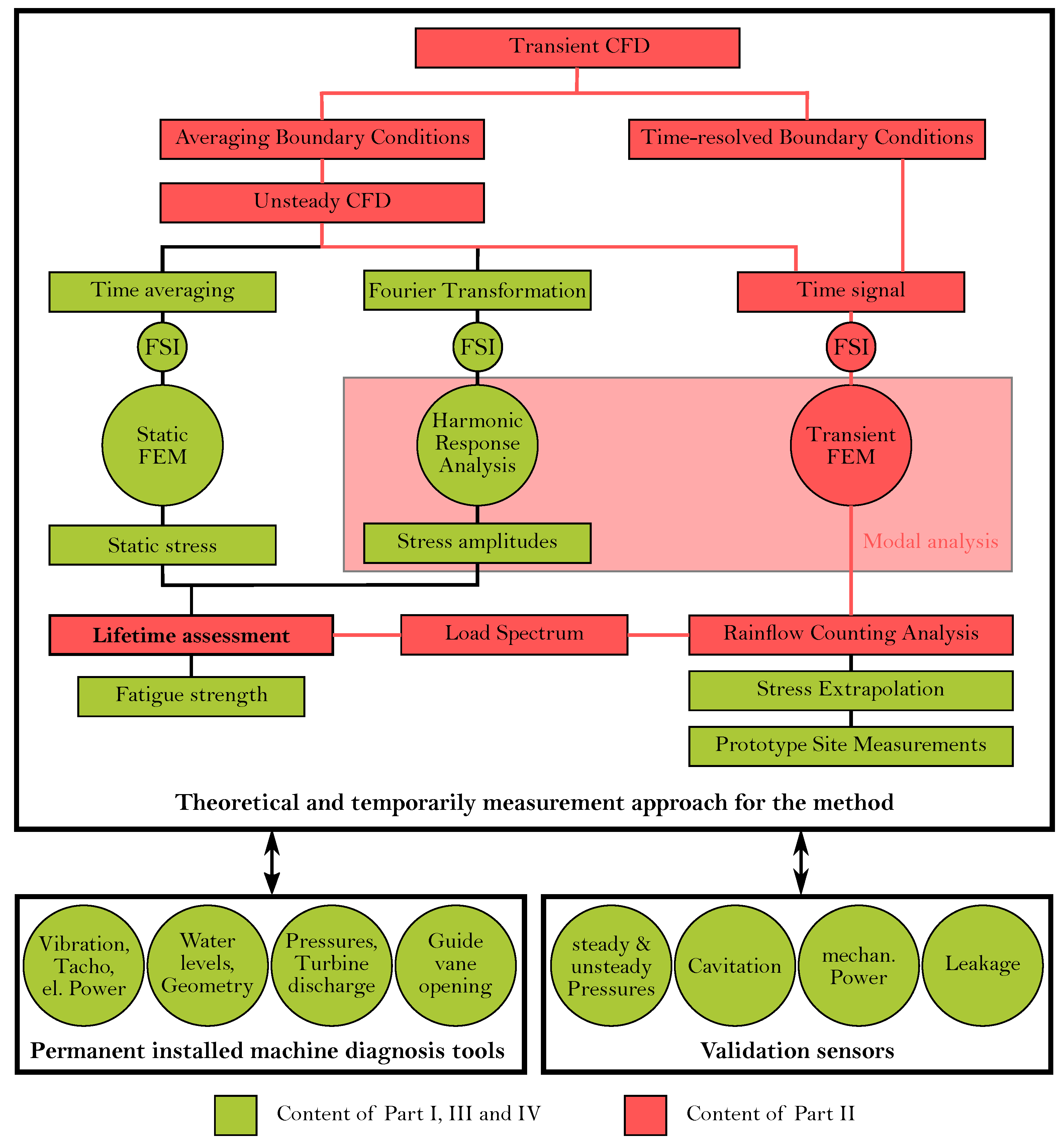
Figure 1 shows the content of this paper in red using the presented assessment protocol. It shows the numerical simulation path from the transient CFD calculations, the fluid–structure interaction, and the mechanical stresses’ calculations down to the lifetime analysis. The paper deals with the necessary models which have to be generated for the calculation. Any uncertainties in the input parameters are discussed utilizing sensitivity analyzes. The accompanying prototype measurements validated the entire simulation approach. Likewise, the sensitivity analyses were estimated accordingly by sensors at the monitor points.

Using numerical methods to determine the lifetime, it is essential to quantify the used methods’ reliability. Ultimately, the determination of systematic errors can be domain-specific (CFD, FSI, FE) or based on the overall comparison of the calculated lifetime to the measured one. This point of uncertainty considerations is further elaborated in PAPER IV. Here, a description of the used turbines is given, followed by the models and their boundary conditions, and finally an application of the simulation models to determine the numerically calculated lifetime on an actual turbine. On the one hand, the data’s evaluation takes place the hotspots because these are failure-critical and thus relevant for the lifetime calculation. On the other hand, at the positions of the strain gauges during the prototype measurement, calibrate the entire calculation method.

The numerical simulation procedure part, which is already used as a standard in the industry, is not explained in detail here due to lack of space. Only those segments of the evaluation process that are not yet part of the industrial design repertoire for Francis turbines’ will be described. This method is still possessed for research projects with the appropriate hardware, computer capacities, and measuring equipment. About 3 million CPU hours were used for the flow calculation of the two Francis runners examined.

2. Description Hydropower Plants and Machine Units

2.1. Pumped Storage Power Plant 1

The first power plant available for this method’s development is a pumped storage plant with a bottleneck capacity of 2 × 180 MW and a regular annual working capacity of 189 GWh. The cavern powerhouse is located 744 m below the upper reservoir. It is connected by the head waterway system, which consists of the intake structure with gates, the subsequent headrace tunnel with surge tank and shut-off device, followed by the penstock, the branch and the turbine closing valve. The plant is equipped with two machine units of the same size. These are pumped storage units based on the 3-machine principle, consisting of a synchronous generator, a Francis turbine, the hydraulic converter and a two-stage single-flow storage pump (see Figure 2). The discharge of the two turbine units is combined via a pipe connection and leaves the powerhouse through the common tailwater channel in the direction of the 70 m higher situated tailwater reservoir.

The turbine section of the machine unit is divided into an upper generator bearing, which is designed as a combined axial thrust and radial guide bearing, the synchronous generator with a speed of 600 min⁻¹, the lower generator radial guide bearing, the intermediate turbine shaft, the upper turbine radial guide bearing, the Francis turbine with a spiral case, stay vanes, guide vanes and draft tube with through shaft, the lower turbine radial guide bearing, the intermediate converter shaft and the hydraulic torque converter, which serves as a coupling between turbine and pump section. The pump section consists of the converter shaft, the upper storage pump radial guide bearing, the multistage storage pump including the intake and the lower storage pump bearing, which is designed as a combined axial and guide bearing. For main machine data see

Table 1. Machine main data.

Machine Main Data	2 Pumped Storage Machine Sets with Francis Turbine, Synchronous Generator and Storage Pump
Head at rated discharge	744 m
Rated power in turbine mode	180 MW
Rated discharge in turbine mode	28 m3/s
Rated generator capacity	212 MVA
Nominal speed	600 min−1
Machine Layout	Vertical Two Machine Setup
Upper generator bearing	Combined axial thrust and radial guide bearing
Generator	Synchronous
Lower generator bearing	Radial guide bearing
Upper Turbine bearing	Radial guide bearing
Turbine	Francis type in metal spiral case with stay and guide vanes
Lower Turbine bearing	Radial guide bearing
Coupling	Hydraulic torque converter
Upper storage pump bearing	Radial guide bearing
Storage pump	Two-stage single-flow storage pump
Lower storage pump bearing	Combined axial thrust and radial guide bearing

.

2.2. Hydropower Plant 2

The selected hydropower plant for the measurements has a bottleneck power of 86 MW and a regular working capacity of 356 GWh. The entire power plant’s components start with the upper reservoir, including an inlet structure with a shut-off device, the attached pressure tunnel with surge chamber and valve followed by the penstock, bifurcation and turbine closing valve in front of the spiral case of the machine unit. The power plant is equipped with two machine units of the same size, consisting of Francis turbine, guide vane apparatus, turbine bearing, lower generator bearing, synchronous generator, and upper generator bearing, which combine the thrust and guide bearing. The water leaves the runner through a draft tube cone followed by the elbow and a diffuser section in the tailwater reservoir’s direction. The powerhouse itself is designed as a shaft powerhouse with a depth of 28 m and an inside diameter of the outburst of 20.6 m. The produced energy passes the transformers and feeds into the 220 kV transmission line attached to the powerhouse (see Figure 3).

Typically, the Francis turbine units consist of a steel spiral case with stay vanes for stability reasons. The next part in line is the guide apparatus with movable guide vanes for discharge control and the subsequent runner. The machine setup, including the nominal data for the runner’s layout point, is shown in

Table 2. Machine main data.

Machine Main Data	2 Francis Turbines with Synchronous Generator
Head at rated discharge	162 m
Rated power per turbine	43 MW
Rated discharge per turbine	34.8 m3/s
Rated generator capacity	53 MVA
Nominal speed	428.67 min−1
Machine Layout	Vertical Two Machine Setup
Upper generator bearing	Combined Thrust and guide bearing
Generator	Synchronous
Lower generator bearing	Radial bearing
Turbine bearing	Radial bearing
Turbine	Francis type

.

2.3. Comparison of Runner Design

The hydropower plants’ selection for the two research projects PSP-LowLoad and MDREST was based on the installed runners. Turbine runners with different characteristics were deliberately selected in order to be able to study differences in their operating behaviour. The main selection features were the specific speed $n_q$, the resulting design, and the labyrinth seals’ arrangement. The position of the labyrinth seals, in particular, is decisive for the axle thrust. These three parameters are briefly described in the following subsections.

2.3.1. Specific Speed

To compare different runner layouts, a specific reference number has to be considered. In Europe, the so-called specific speed is prevalent. The definition of this reference parameter depends on similarity rules and the equation:

$$n_q=n_A\frac{\sqrt{Q_A}}{{\left(H_A\right)}^{\frac{3}{4}}}\frac{{\left(H_q\right)}^{\frac{3}{4}}}{\sqrt{Q_q}}=n_A\frac{\sqrt{Q_A}}{{\left(H_A\right)}^{\frac{3}{4}}}\frac{{\left(1\mathrm{m}\right)}^{\frac{3}{4}}}{\sqrt{1{\mathrm{m}}^3/\mathrm{s}}}\left[{\min }^{-1}\right]$$

(1)

with the runner speed $n_A$ in min⁻¹, the rated discharge $Q_A$ in m³/s, specific discharge $Q_q=1{\mathrm{m}}^3/\mathrm{s}$ and the head at rated discharge $H_A$ in m, specific head $H_q=1$ m.

Table 3. Machine layout data and specific speed.

Machine Layout Data	Machine 1	Machine 2
Net head at rated discharge	629.3 m	137.51 m
Rated discharge per turbine	28 m3/s	34 m3/s
Nominal speed	600 min−1	428.67 min−1
Specific speed	25.4 min−1	62.2 min−1

shows the resulting values for the two investigated runners.

Based on the values in Table 3, two different runner designs are the result. The first runner has an $n_q$ of 25.4 min⁻¹ and is therefore expected to be very radial, while the second runner has an $n_q$ of 62.2 min⁻¹ and hence larger, wider blade channels.

2.3.2. Design

Looking at the two runners in more detail, one can observe that the runner with the smaller $n_q$ has the following design characteristics: an inclined but straight leading edge of shallow height, a narrow blade channel that runs very radially, and in the last third it is widened in the direction of the axial outflow. The blades themselves are twisted and have a curved trailing edge. The hub diameter inside is larger because, in this particular case, a through shaft is installed. The number of shroud-side labyrinth seal chambers indicates a very high head. In the second case, we already see some double-curved leading edge, which has a much greater inlet height. The blade channel is much more spacious, and the blade itself is also shorter. The trailing edge is single curved and has a considerable height. The hub, in this case, is designed as an open hub, as the ventilation during condenser mode operation takes place through this part of the runner. The arrangement of the labyrinth seals and their chambers are discussed in the next chapter.

The CAD design of the two runners is shown in Figure 4.

The two wheels examined differ in their characteristics and were therefore selected. Seidel et. al. found in [31] that the specific speed $n_q$ has a significant influence on the RSI. The same behavior is expected here.

2.3.3. Runner Sealing Position

Looking at the labyrinth seals of the two selected runners, the following differences were observed: the left-hand runner with the lower $n_q$ has two fir-tree shaped gap labyrinths on the hub side and several seal chambers on the shroud side at the end of the runner sidewall gap in the direction of the draft tube. In the right meridian section of the runner with the higher $n_q$, the labyrinth seal chambers are located on the runner’s outer diameter, nearly in the same cylinder plane. Figure 5 shows the positions of the labyrinth seals in the respective meridian section of the runner.

The essential difference is that in the left runner of Figure 5, the pressure reduction on the hub side occurs at about half the runner diameter. The pressure reduction on the shroud side occurs at the impeller outlet at the end of the runner’s side chamber. This means that large parts of the runner are affected by headwater pressure, which means a positive effect on the blade stresses at the leading edge due to $F_{DOWN}=F_{UP}$, and the axial thrust is reduced.

The right runner of Figure 5 has the labyrinth seals on the outer diameter of the runner, and reduces the pressure there to tailwater level. This means, that this runner has to cope with the entire blade channel pressure and the full turbine head in terms of stress. However, the advantage for the sidewall gap pressure distribution here is that the pressure due to the head is directly reduced at the beginning of the axial part of the sealing, thus resulting in a lower pressure distribution at the turbine hub. Otherwise considerable axial thrust would appear, since the resulting force due to the pressure distribution at the turbine shroud does not counteract with the resulting force at the turbine hub ($F_{DOWN}\ne F_{HORIZONTAL}$).

3. Numerical Simulations at the Transient Assessment Model

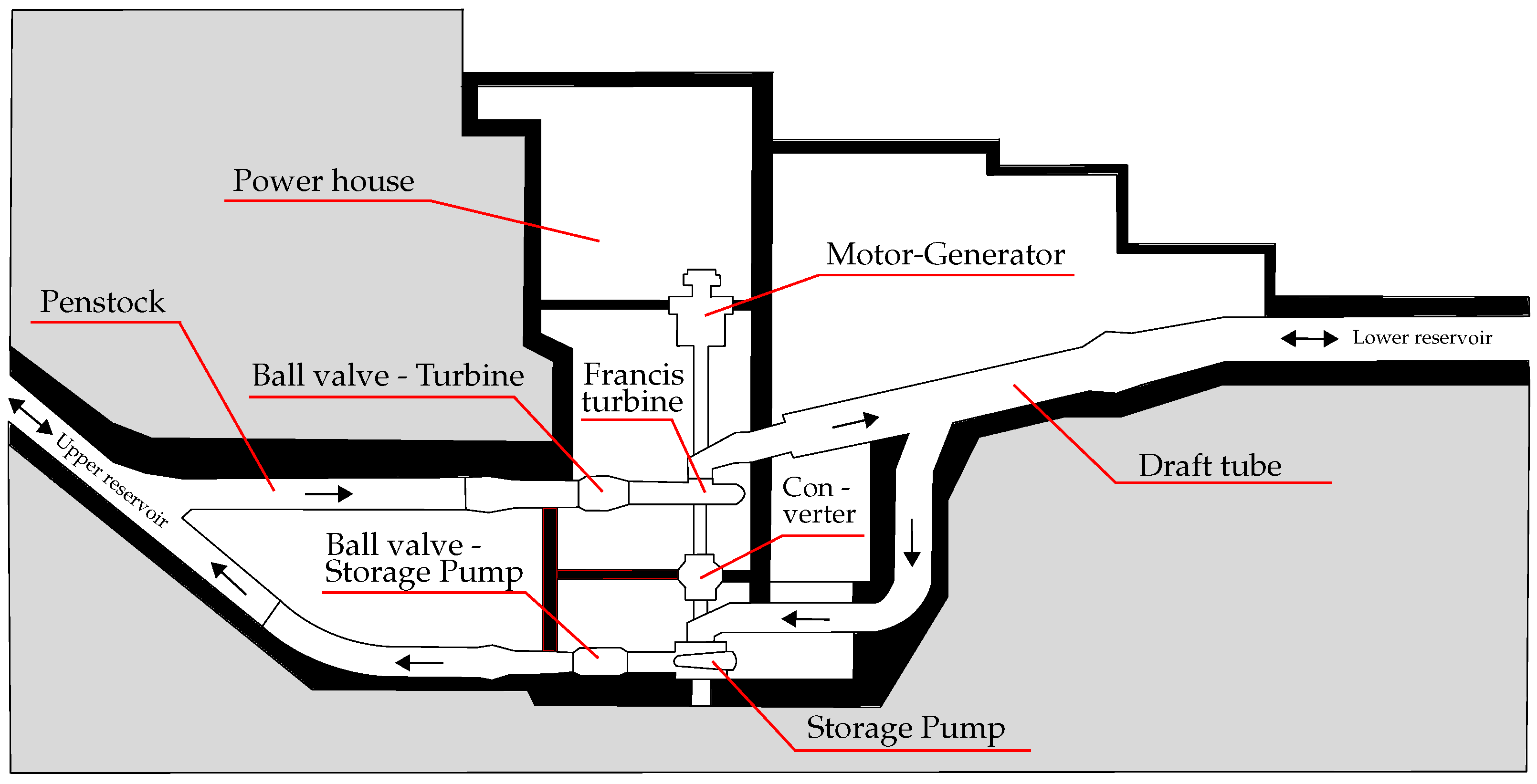
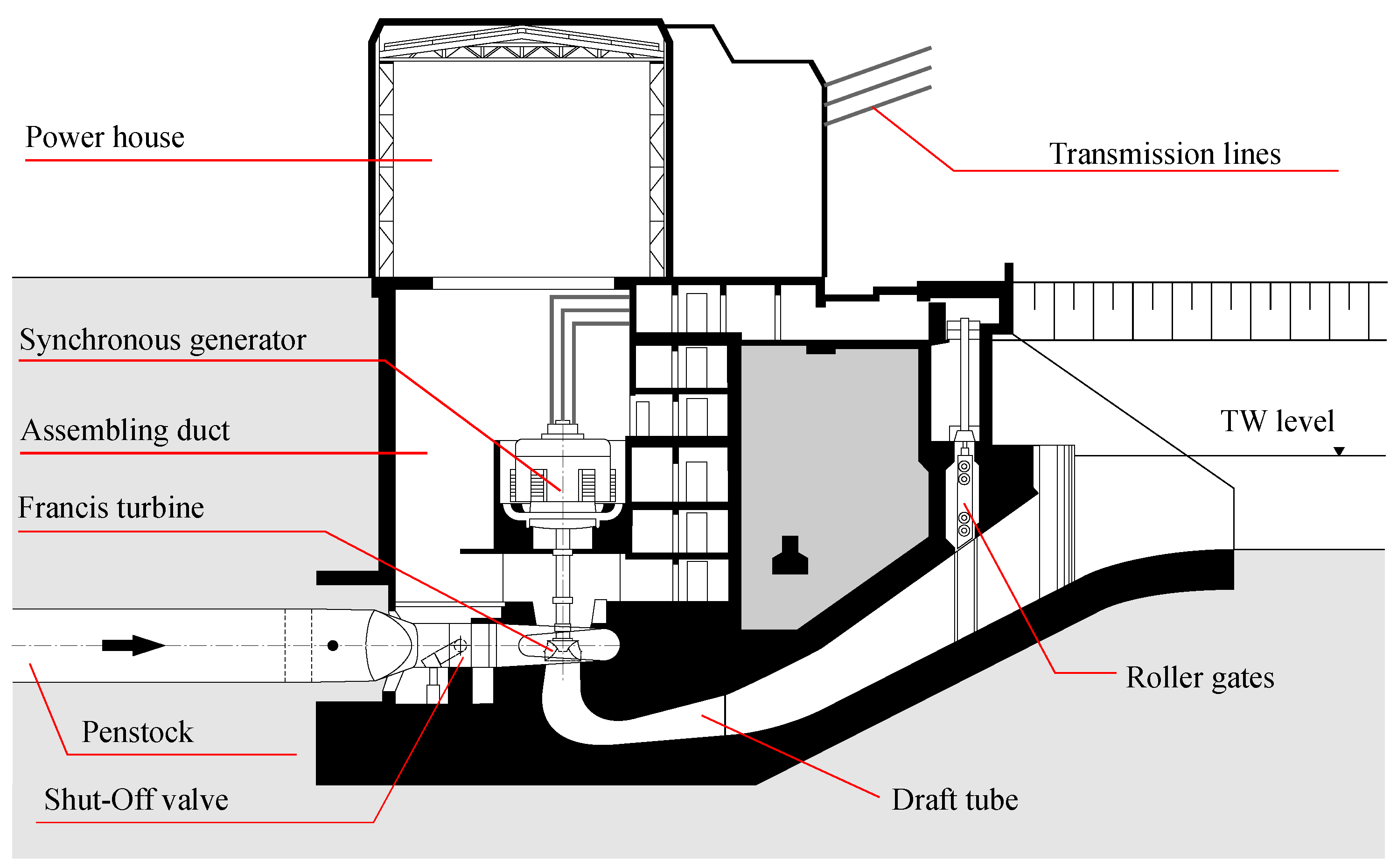
This chapter’s further explanations include only hydropower plant 2, although they can be transferred to the pumped storage power plant 1 analogously. Lack of space prevents the authors from presenting the detailed modeling of both plants. In cases of significant differences that might lead to different solutions, they are mentioned accordingly. The method used remains unaffected and can be transferred.

Section 3 illustrates all computational models, boundary conditions, and input parameters necessary to conduct the lifetime’s numerical determination. Details have already been published on several occasions. Therefore only a brief description of the principal but essential parts like CFD, FEA, and Modal analysis are given.

Where boundary conditions or input parameters were not available in the appropriate accuracy, sensitivity analysis, including measurements by validation sensors, was performed. Hence, it became possible to investigate how dependent the results are on the assumed or underlying parameters. These uncertainties will be addressed and further explored in Part IV of this publication series. An important point will be the interaction of various uncertainties and deviations on the final result, the mechanical stress in the runner, or its lifetime.

3.1. Computational Fluid Dynamics (CFD)

As shown in Figure 1, the numerical flow simulation is the evaluation method’s initial point. The procedure steps themselves have already been described [32] and are not discussed further. This chapter deals with the models, boundary conditions, and limitations.

3.1.1. Model Description

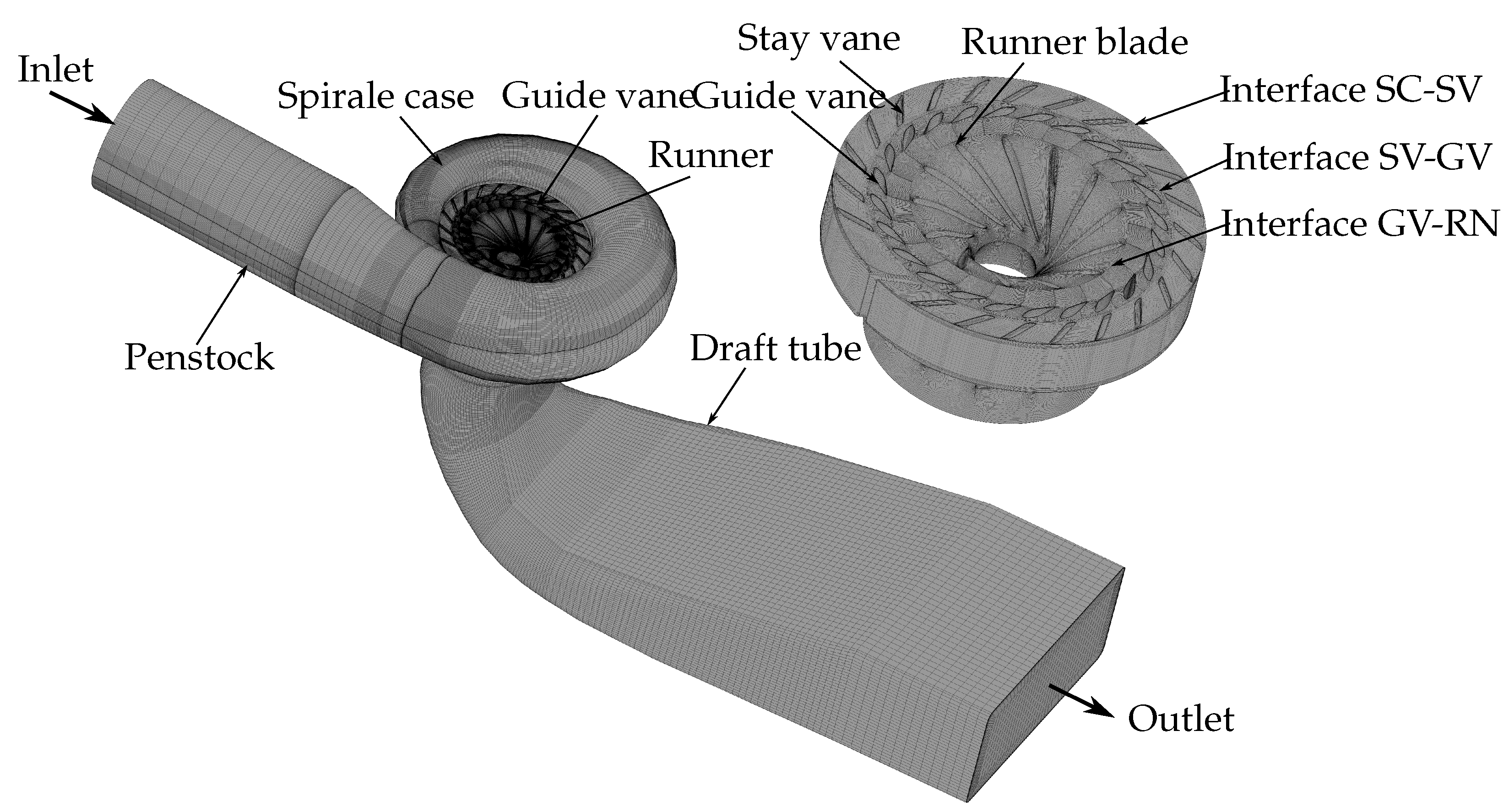
As both transient and unsteady calculations are carried out, no symmetry conditions can be used to discretize the fluid domain. Accordingly, the full model of the hydraulic turbines consists of:

• Connection to the penstock;
• Spiral casing;
• Stay vane ring;
• Guide vane;
• Runner;
• Draft tube.

The individual meshes of the components are afterward coupled by interfaces (see Figure 6).

The mesh discretization of the individual components followed general guidelines. The entire mesh of the machine was then subjected to a mesh independency study according to [33]. Different mesh refinements were generated for different studies in order to resolve the respective flow effects. Parameters such as wall spacing, wall treatment, Y+, and more were adjusted to the turbulence models used. For example, grid sizes of about 6 million cells were used for the investigation of transient processes in the low-load region [30] for hydropower plant 2. In the case of transient processes (e.g., STU), a mesh with approximately 13 million cells [34] was created and for the investigations of air injection and vortex shedding at the trailing edge of the runner, the existing mesh had to be refined again to approximately 37.5 million cells [35].

In terms of pumped storage plant 1, the mesh was created from individual meshes and coupled by interfaces. The entire machine unit consisted of approximately 6 million elements [36]. Flow parameters and grid independence study were performed accordingly.

3.1.2. Boundaries

In terms of boundary conditions and requirements for the model, the following settings should be considered:

• The global boundary conditions (inlet and outlet) should never be set at those surfaces where an evaluation plane or monitor points (=measurement points) are located, but always beyond.
• The inlet is determined as mass flow rate, whereas the outlet consists of a static pressure level. This combination proved to be numerically stable. Furthermore, the mass flow and the pressure at the draft tube outlet are adapted to the actual measured values.
• In the case of pumped storage power plant 1, a radial pressure equilibrium was set at the draft tube outlet due to a circular cross-sectional shape at this area. This setup results in more realistic values, especially in the low-load range. The calculated values were compared with the measured ones at this point.
• The coupling of stationary interfaces is modeled by a General Grid Interface (GGI). For the rotor-stator interaction, a transient rotor-stator interface, implemented in Ansys CFX 18.0, is used for the unsteady analysis.
• To capture transient events, an approach covering moving guide vanes and varying boundary conditions is presented in [30]. The guide vane movement is realized by using a displacement diffusion model combined with a re-meshing procedure, which is further explained in [37].
• As fluid, water at 20 degree celsius, treated as single-phase incompressible medium, is used for general investigations. In terms of air injection a two-phase model in combination with a cavitation model was used.

3.1.3. Turbulence Model

The selection of the supposedly correct turbulence model for calculating a wide variety of off-design points evolved.

In terms of steady CFD analysis, the shear stress transport (k-$\omega$-SST) model is used while in case of the unsteady analysis the SAS-SST model is preferred [28]. To ensure sufficient convergence, 1000 iterations with a physical time step of $1/\omega$, which corresponds to one runner rotation, are simulated. In case of the unsteady analysis. In case of the unsteady analysis the time step is set to a value corresponding to $1^{\circ }$ of one runner rotation The results of the steady state simulation are used as an initial condition to improve and speed-up convergence. Furthermore, a total amount of 15 runner rotations were simulated.

At the Start-Up (STU) simulations a new turbulence model was used, namely the Stress Blended Eddy Stimulation (SBES) turbulence model. An approach which combines strong shielding and protection against the LES application in the boundary layer as well as WMLES. The model provides rapid and distinctive RANS-LES transition.

3.1.4. Numerical Simulation Program

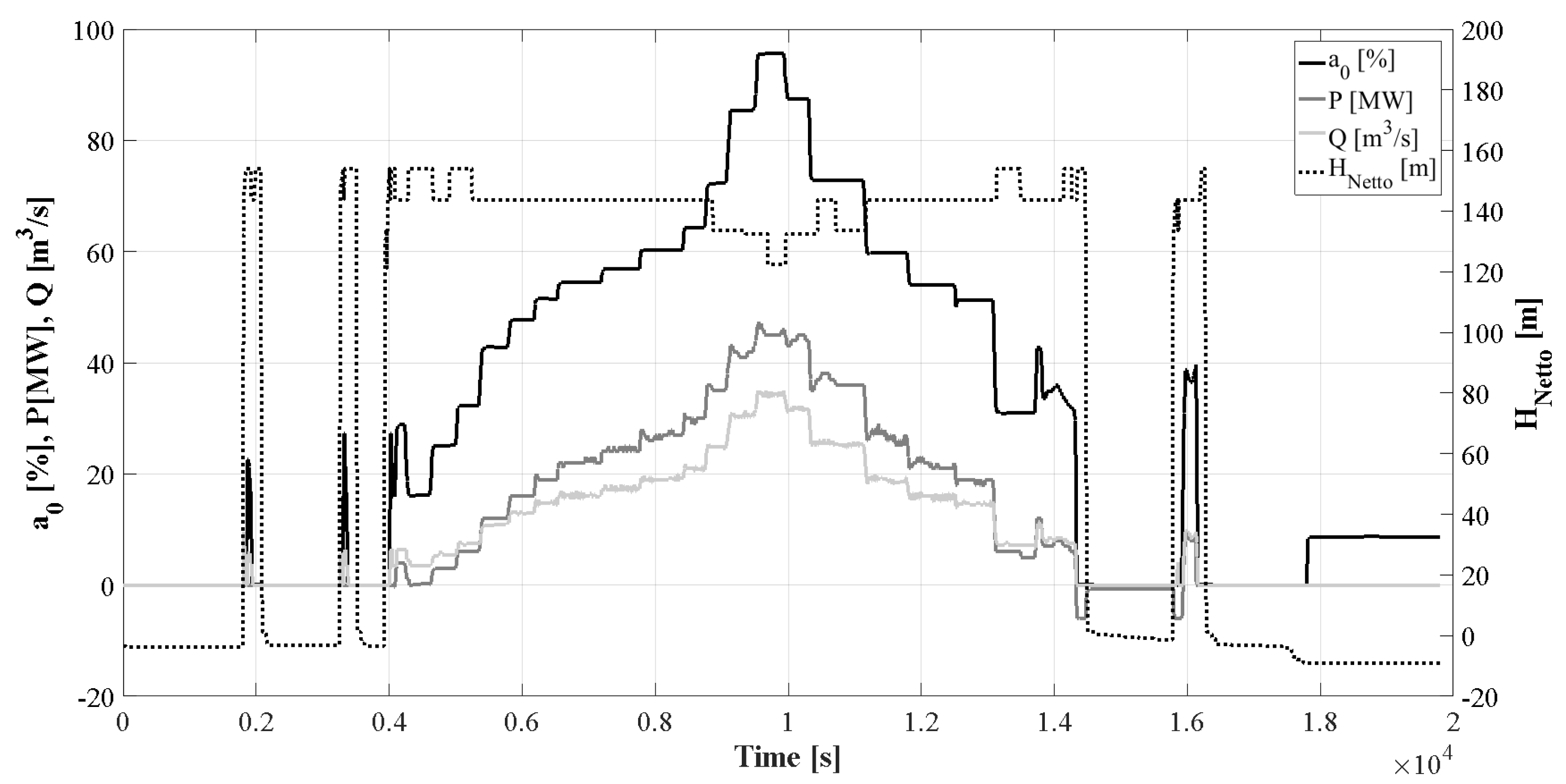
The numerical simulations follow the prototype measurements. Such a procedure is the only way to ensure that the calculations are based on real boundary conditions and validation values.

The numerical simulations have been performed according to Figure 7. Start (STU) No. 1, at approximately $0.2\times {10}^4$ s, and Start (STU) No. 2, at approximately $0.35\times {10}^4$ seconds of the machine unit were investigated and published by [37]. Furthermore, the load rejection (LR) case, at approximately $1.6\times {10}^4$ s was investigated. These operating points are also called transient operational points because they are extremely unstable in terms of flow behavior, and phenomena can occur momentarily and disappear again.

In contrast, with the machine already synchronized, the load changes represent relatively stationary operating changes. Reference [38] investigated all load changes concerning their effects on the dynamic stresses, using the transient pressure field calculations, from the low partial load point to the overload, as a starting point.

3.2. Modal Analysis (Natural Frequencies/Eigenmodes)

In addition to the apparent exciting frequencies like the runner’s rotational speed, there is a bunch of other phenomena in hydropower turbines, which can excite parts of the machine. Phenomena like the gate passing frequency, vortex shedding, or the draft tube vortex are well known and determined with numerical methods. This makes it even more important to know the components’ natural frequencies, which can potentially be excited. The following chapter should show some possibilities to capture the natural frequencies of important machine parts.

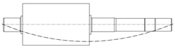
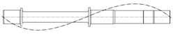
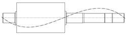
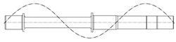
3.2.1. Guide Vane

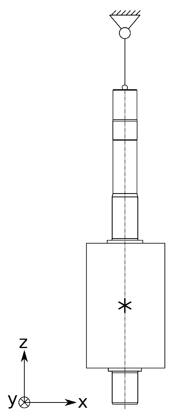
Two different guide vane models were used for the modal analysis of this part. The first model was intended to represent the free-swinging guide vane, and hence it had no supports as shown in Figure 8. The rigid-body modes resulting from this boundary condition are ignored for further evaluation of the results. The second model represented the guide vane in its mounted configuration. For this, guide vane struts and the three bearings were considered. Due to the lack of reliable bearing data, no velocity-dependent damping could be used, but instead, the simpler model of Rayleigh damping. The two parameters necessary for Rayleigh damping were determined using the damping ratio $\theta$ derived from the measurements.

3.2.2. Runner

The following section contains the description of the used models, boundary conditions and restrictions or dependencies.

• Description of model
  For the runner’s modal analysis and the further evaluation of the added mass effect, a reference model (Model 1) and two models with different approaches of water volume modeling were created. Model 1 incorporates a runner in air investigation and serves as a reference for further comparisons. The runner in a water tank model (Model 2) is the first benchmark to investigate the added mass effect. On that occasion, a simple water cylinder was placed around the runner (see Figure 9), which accords the infinite large water tank.
  Moreover, the second model considered a limited area at the intake, a small part of the draft tube, and the runner sidewall gaps (see Figure 10). In the following, this setup is referred to as Model 3. Other configurations have been investigated but will not be discussed further as this would exceed the limits of this paper. A detailed description can be found in [39].
  These models used the same boundary conditions: fixed support at the runner crown, no external forces, and no structural damping. The water volume was meshed with FLUID221 elements; the water volume’s mesh size was a sixth of the wavelength of the highest frequency of interest (for quadratic elements). For linear elements, a twelfth would be necessary. On surfaces with no pressure wave reflection a fixed pressure boundary condition was applied. Referring to the cylinder-model, these are all outer faces of the water volume. At the runner sidewall gap model, these are the inlet and outlet faces. All other faces, which are no FSI, reflect the pressure waves without any losses.
• Boundaries/effects
  To determine the added mass effect on the runner’s natural frequencies, the runner’s modal analysis in air was compared with the results of the cylinder model. The first finding is based on the fact that the volume of water generally lowers the natural frequencies. Furthermore, one observes that the added mass has different influences on the varying modes. A general conjecture might be that the more fluid has to be agitated through the mode, the stronger the influence on the natural frequencies.
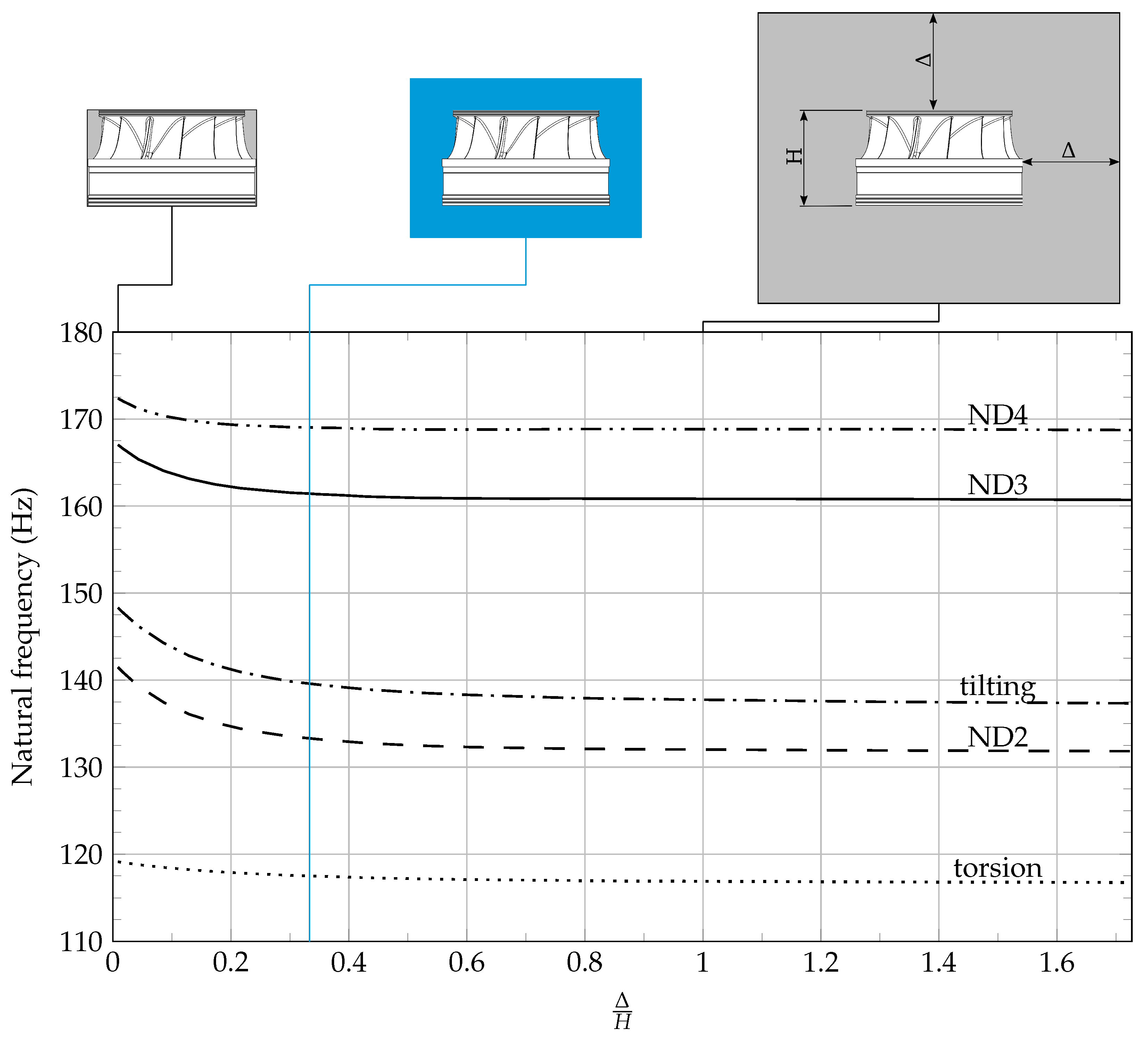
  In a second step, the influence of the cylinder-size should be investigated. Therefore the modal-analysis was performed with various sizes of the water cylinder. Figure 11 represents the result that the water masses around the runner affect the natural frequencies only to a specific size. Above this value, the impact of the added mass effect will not change.
  Figure 11 has a practical influence of modeling such cases. If the surrounding volume is to low the results are not independent anymore but calculation time will be lower. On the other hand, very large water volumes will only extend the calculation time whereas the result will not increase accordingly. To balance water volume, respectively, mesh size and simulation time it is necessary to know the limits. If $\Delta /H<0.3$ the failure would be quite high.
• Restrictions/Dependencies
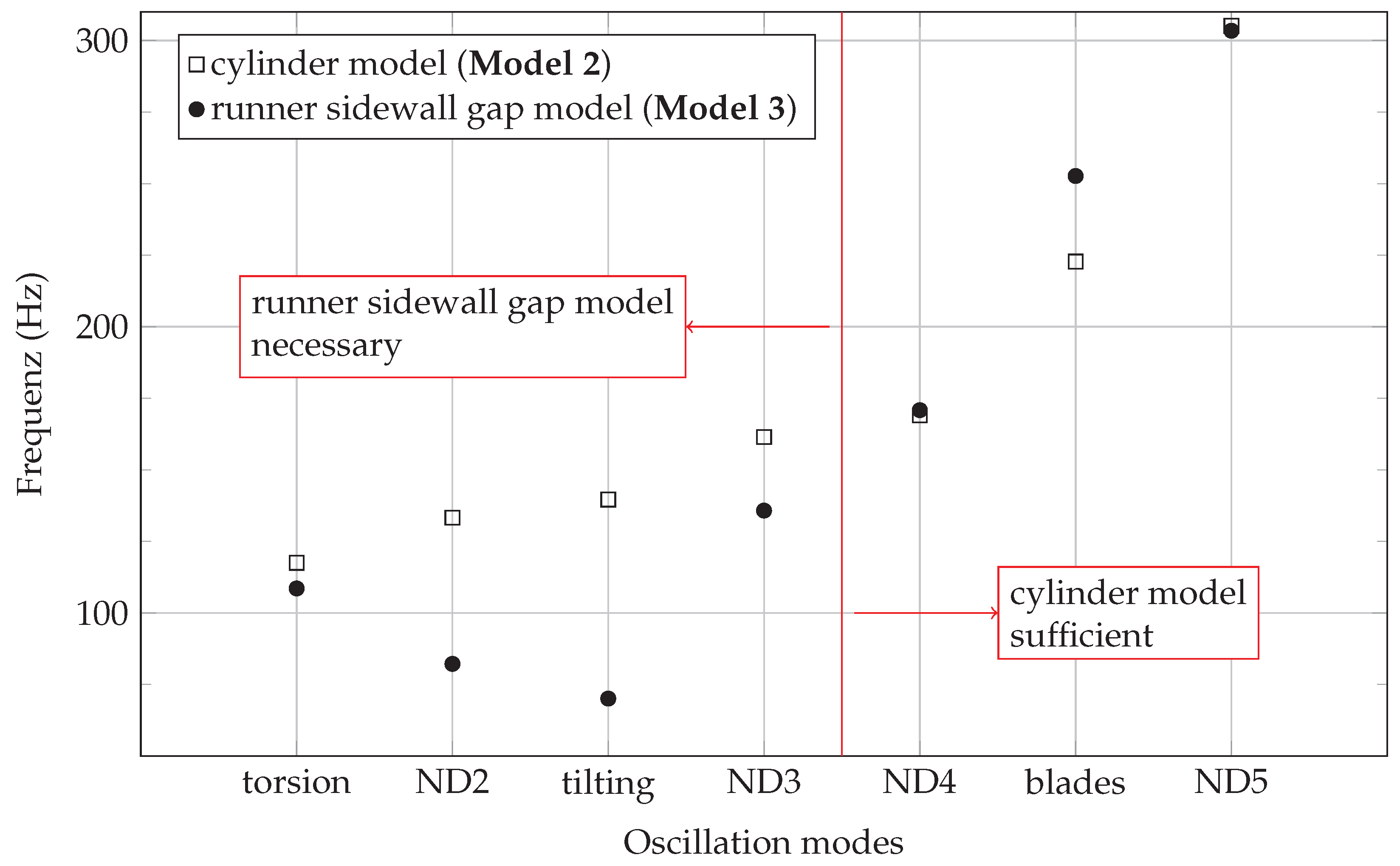
  Figure 12 shows the impact of the added mass effect on the runner related to the oscillation mode. For nodal diameter (ND) modes, one can conclude that concerning $ND=3$ or less, it is necessary to use runner sidewall gap model (Model 3). For modes with $ND=4$ or more, the cylinder model (Model 2) is sufficient. The explanation is based on the fact that higher nodal diameter modes fulfil a smaller structural displacement, and therefore the impact of the small gap decreases.

3.2.3. Draft Tube

• Description of model
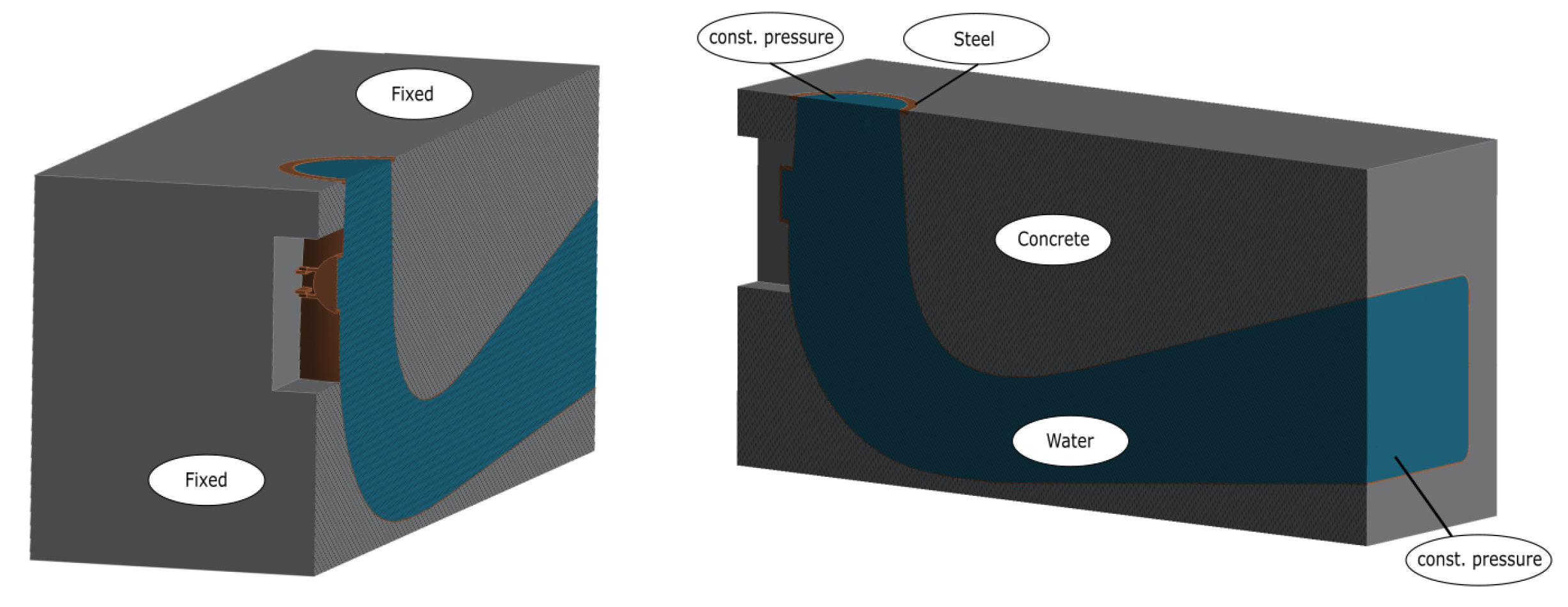
  To determine the natural frequencies of the draft tube a model with three parts (see Figure 13) was used, e.g., the draft tube (red) itself, the enclosed water volume (blue) and the surrounding concrete (grey) foundation. As the entire model consists of solids and liquids an acoustic element approach was selected. The used material parameters and element types for each part are shown in

  Table 4. Summary of materials and element types.

  Component	Material	Density	E-Modulus	Poisson Number	Element Type
  Water volume	Water	1000 $\frac{\mathrm{kg}}{{\mathrm{m}}^3}$	not available	not available	FLUID221
  Draft tube	Steel	7850 $\frac{\mathrm{kg}}{{\mathrm{m}}^3}$	2.1 × 10${}^5\frac{\mathrm{N}}{{\mathrm{mm}}^2}$	0.30	SOLID187
  Concrete foundation	Concrete	2300 $\frac{\mathrm{kg}}{{\mathrm{m}}^3}$	3 × 10${}^4\frac{\mathrm{N}}{{\mathrm{mm}}^2}$	0.18	SOLID187

  . Boundary conditions on the concrete foundation’s outer side remain fixed (translation and rotation fixed) conditions. This assumption is reasonable since the model only displays a section of the entire rigid plant. Between the concrete foundation and the steel-lined draft tube, a bonded contact was chosen. Since the water and steel domain use different element types, the importance of conforming meshes is obvious. The conforming mesh is needed for the Fluid-Structure Interface (FSI) in that way that forces and displacements can be exchanged easily between the domains. Constant pressure was applied at the involved outlet of the fluid domain.
  Even if Figure 13 might suggest using only half of the model and placing symmetry conditions at the cutting plane instead, this option was not used, as information loss about possible eigenmodes and wrong calculated natural frequencies could occur. The mesh consists of quadratic tetrahedral elements SOLID187 for the concrete and draft tube part, whereas FLUID221 elements were used for the water volume. The element size for the water volume was selected according to the wavelength of the highest frequency of interest. Internal rules suggest an element size being at most a sixth of the wavelength.
• Boundaries/effects
  • Added mass effect
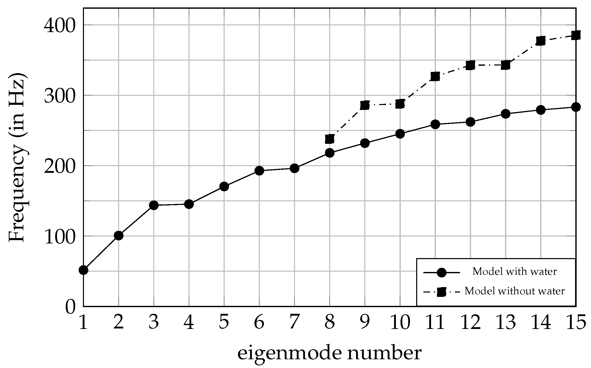
    Determining the effect of the added water volume on the natural frequencies needed two simulations to be run. One with the enclosed water volume and one without it. Figure 14 shows the natural frequency related to the eigenmode number. One can observe that the natural frequencies of the model with water start at a noticeably lower frequency. This model’s first eigenmode is found at 51.75 Hz compared to a model without the water volume having its first natural frequency at 238.97 Hz.
    As the mass of the model with water is more significant than without it, the natural frequencies get substituted. This effect was called added mass effect and was first found by Stokes in 1851.
  • Mesh size effects
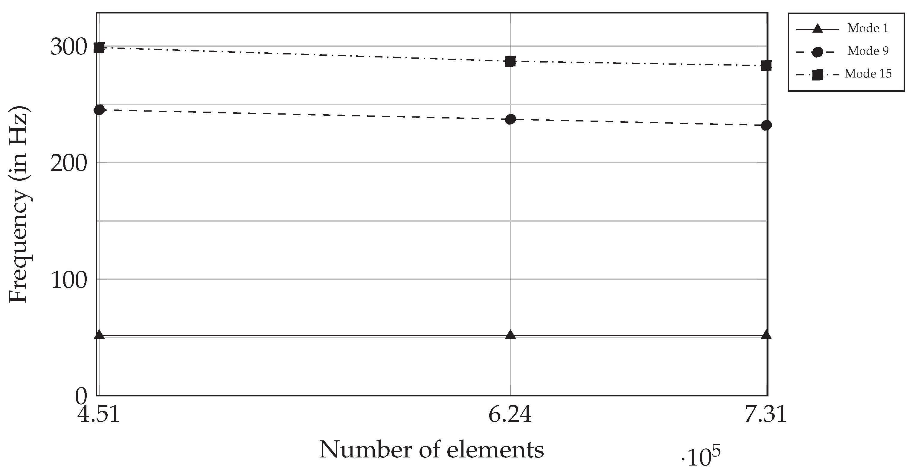
    A mesh independency study ensures that the results do not rely on the mesh size. Different mesh sizes and results are shown in

    Table 5. Mesh indepence study.

    Input Parameters	Model 1	Model 2	$\pm {\Delta }_{1–2}$	Model 3	$\pm {\Delta }_{2–3}$	$\pm {\Delta }_{1–3}$
    Element size of Water volume (in mm)	300	250	−16.67%	230	−8.00%	−23.33%
    Element size of Draft tube (in mm)	95	80	−15.79%	70	−12.50%	−26.32%
    Element size of Concrete foundation (in mm)	460	420	−8.70%	400	−4.76%	−13.04%
    Nodes	451,279	623,916	+38.26%	731,332	+17.22%	+62.06%
    Elements	300,547	417,364	+38.87%	488,133	+16.96%	+62.41%
    Simulation time (in min)	20	31	+55.00%	34	+9.68%	+70.00%
    Evaluation
    eigenmode 1 (in Hz)	51.78	51.76	−0.04%	51.75	−0.02%	−0.06%
    eigenmode 9 (in Hz)	245.32	237.26	−3.29%	232.04	−2.20%	−5.41%
    eigenmode 15 (in Hz)	298.78	287.02	−3.94%	283.29	−1.30%	−5.18%

    and plotted for three eigenmodes in Figure 15. The interpretation shows that lower natural frequencies result in a lower impact on the mesh size. With increasing frequency, the solution gets more sensitive to the mesh sizing. Due to memory constraints on the workstation, a tighter mesh could not be simulated. Although a smaller mesh size would be required to show a better convergence, the decreasing tendency leads to a convergent consideration.
  • Boundary influence of the concrete section width
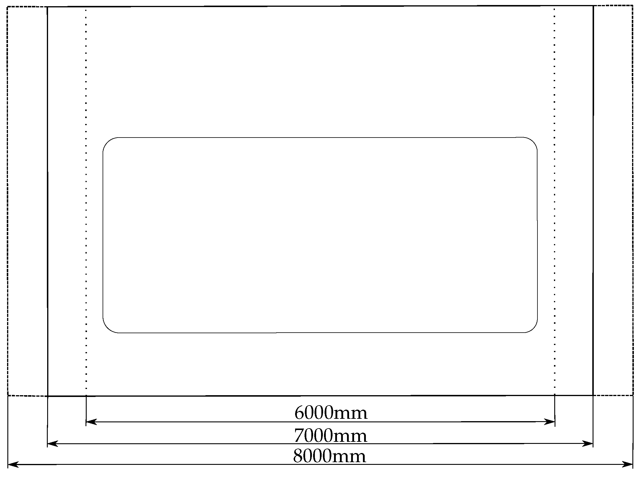
    Modeling the steel casing including the attached parts, the influence of the concrete foundation on the natural frequencies of the draft tube exit was considered by a sensitivity analysis. As the concrete foundation connects to other parts of the power plant, the width plays a vital role. To answer this question, three different models (see Figure 16) with widths of 6000, 7000 and 8000 mm were simulated, and the first 15 natural frequencies evaluated. Out of the 15 natural frequencies, only three, namely 1, 9 and 15, were taken into account for further reflections. The results can be found in

    Table 6. Concrete influence study.

    Evaluation	Model 1	Model 2	$\pm {\Delta }_{1–2}$	Model 3	$\pm {\Delta }_{2–3}$	$\pm {\Delta }_{1–3}$
    Total width (in m)	6	7	16.67%	8	14.29%	33.33%
    eigenmode 1 (in Hz)	51.95	51.75	−0.38%	51.65	−0.19%	−0.58%
    eigenmode 9 (in Hz)	232.19	232.04	−0.06%	232.07	0.01%	−0.05%
    eigenmode 15 (in Hz)	288.54	283.29	−1.82%	283.37	0.03%	−1.79%

    . The width of the draft tube exit has no significant influence on the lower natural frequencies and eigenmodes. This changes with higher eigenmodes as Table 6 shows. The reason could be the stiffness of the material.
  • Influence of the draft tube access area
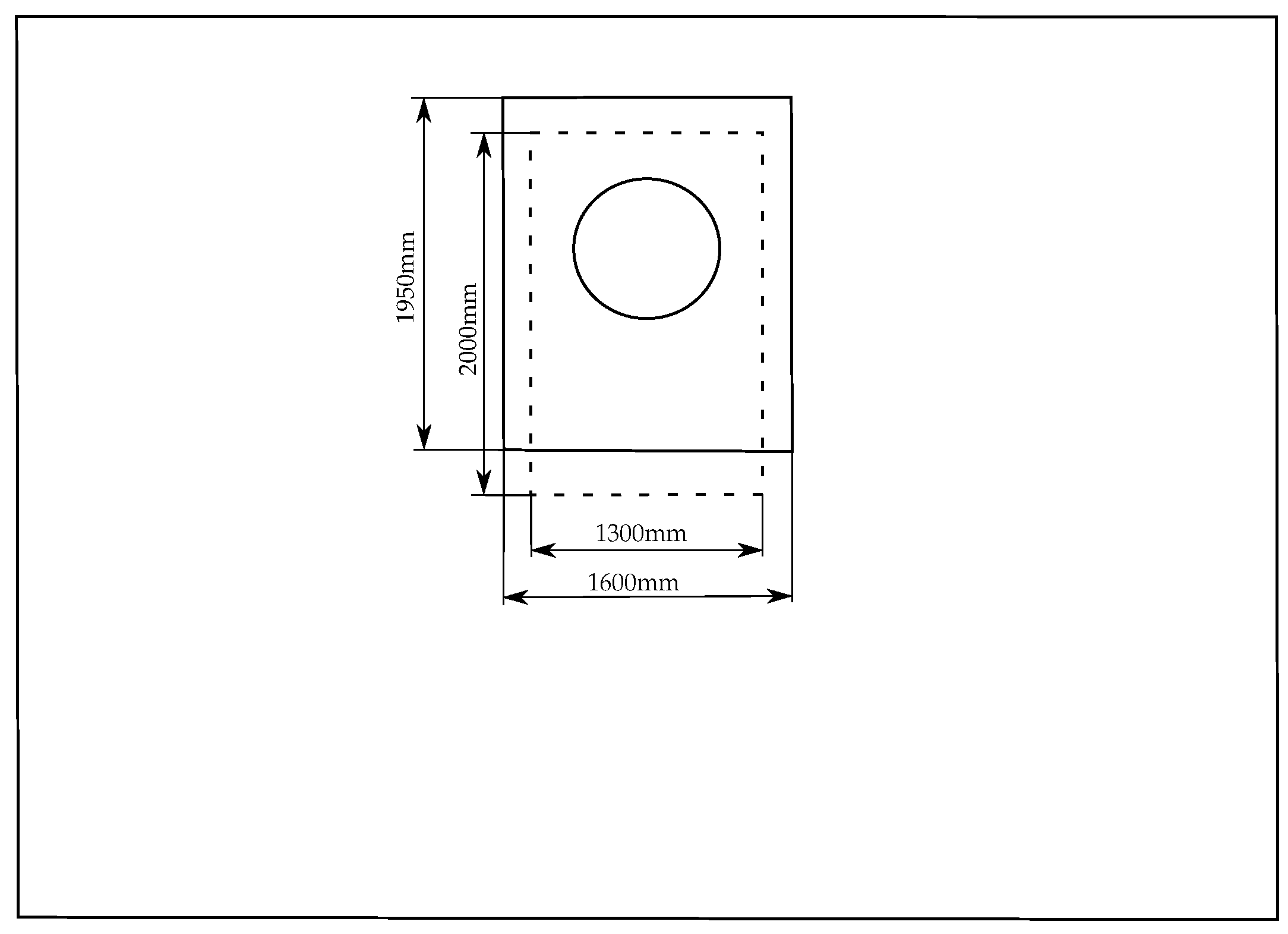
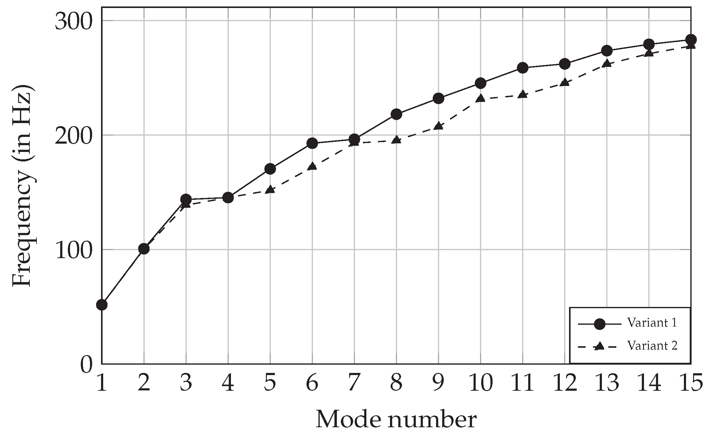
    As the draft tube access area giving way to the maintenance hole cover is an essential part of the concrete foundation, a variation was investigated. Two models with different positions and dimensions were simulated. Figure 17 illustrates the difference between the two models. The solid line shows variation one and the dashed line variation two. The frequencies of the respective modes are plotted in Figure 18. One can see that the difference is negligible in the first four modes. As the frequency increases, the difference becomes bigger and bigger. The largest difference between the two models is 12.4% at mode 8.
• Restrictions/Dependencies
  As seen before, the concrete width and the draft tube maintenance hole’s access geometry influence the natural frequencies of the draft tube. The access area’s geometry is essential since it can lead to significant deviations of the natural frequencies. Therefore one should be very careful at creating the model as realistically as possible in terms of dimensions and positions.

3.3. Finite Element Analysis (FEA)

To numerically record the effects of occurring flow phenomena on the runner’s structure and lifetime for the entire operating range of the hydropower plant 2, from low partial load to overload, transient CFD-simulations were coupled with transient FE-simulations (see Figure 1). For this purpose, the program ANSYS Mechanical Version 2019 R3 was used to perform separate transient simulations for each operating point between $P/P_{RP}$ = 7–105%. The chosen simulation length corresponds to 5 runner rotations at a defined step size of 3 degrees. Occurring damping effects were taken into account according to [30,40] using the simplified approach of Rayleigh damping.

3.3.1. Description of Model

The general procedure and setup for model construction and meshing has already been published in [28,35,41] and was carried out analogously. The mesh consists of quadratic tetrahedral elements with about 0.6 million nodes. As with Eichhorn [41], only one of the runner blades received an additional local mesh refinement, especially at the transition to the runner hub and shroud, at the leading and trailing edges and around the defined strain gauge positions. 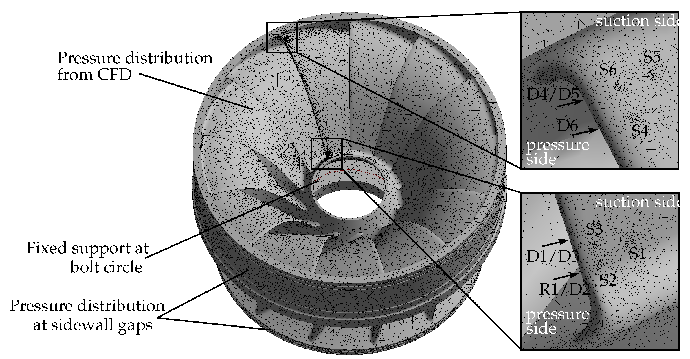For validation of the FE-model, the stresses obtained from the strain gauge measurements, shown in PART III of this publication series and [42], are used. For this reason, the simulation model includes evaluation surfaces with an analogous position, orientation and dimensions of all strain gauges used during measurements (see Figure 19). The mechanical data of the runner material X5CrNi13-4 are Young’s modulus E = 216,000 N/mm², Poisson’s ratio $\nu$ = 0.3 and density $\rho$ = 7700 kg/m³.

3.3.2. Boundaries

In addition to the meshed structure, material properties and computational resources, the following boundary conditions (see Figure 19) are required for the successful realization of the numerical simulations:

❶

Pressure distribution from CFD

The pressure loads determined by transient CFD simulations at each load step are applied to the runner as a boundary condition using unidirectional fluid–structure coupling in the FE analysis. As the fluid and structure meshes at the coupling interface differ, triangulation (see Part I, Section 3.1.2) was used for data interpolation between the nodes.

❷

Pressure distribution at sidewall gap

The pressure distributions were analytically calculated according to Paulitsch [43], based on Gülich [44], and were applied to the FEA model. The methodology itself was investigated and validated at a laboratory model runner [45].

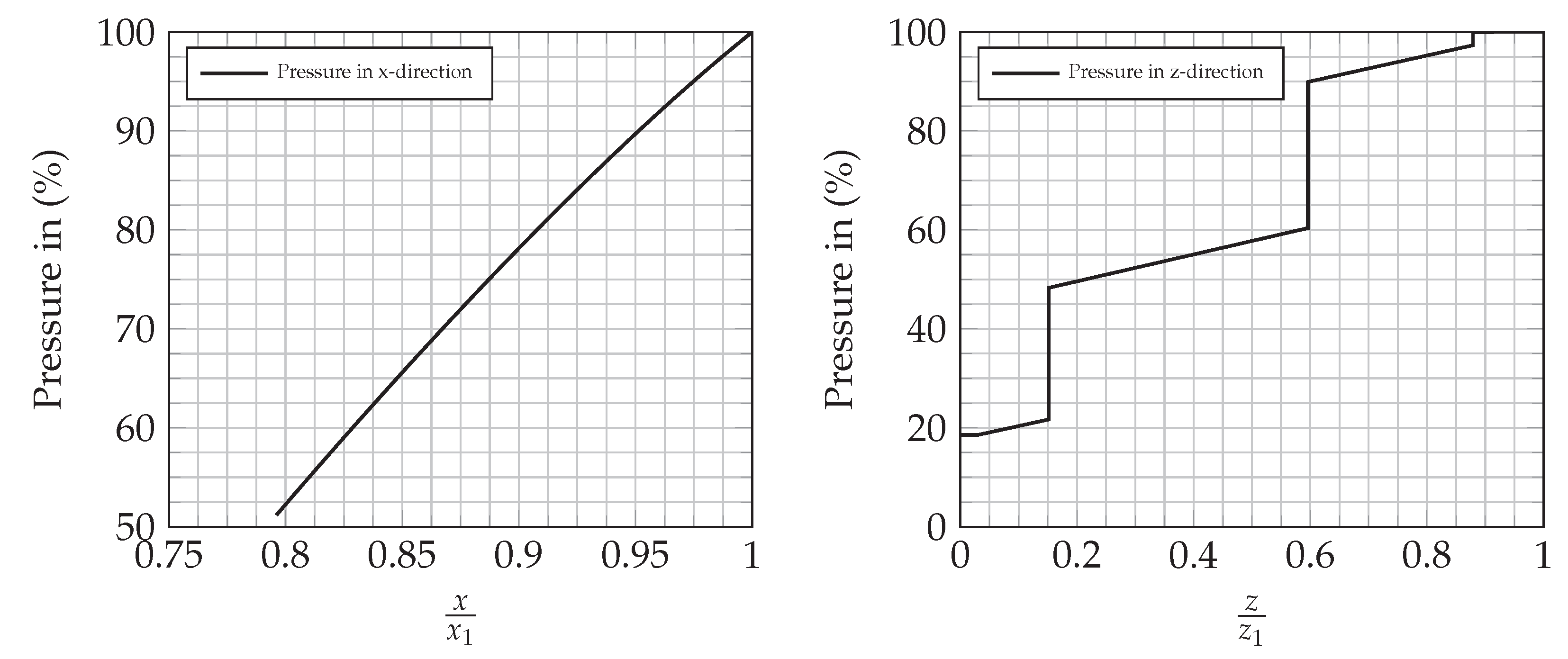
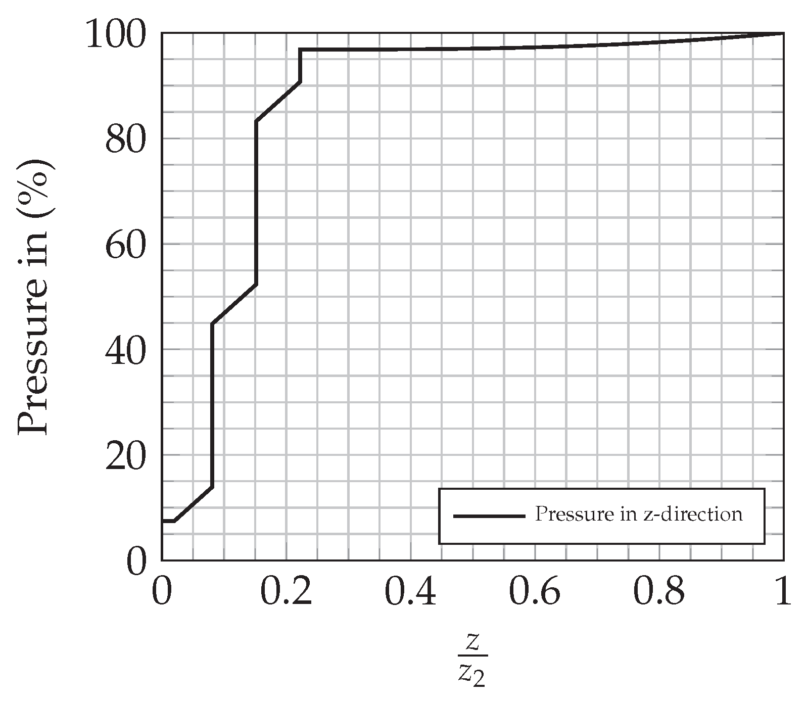
Figure 20 and Figure 21 show the pressure distribution of the runner’s shroud and hub sidewall gaps in hydropower plant 2. The pressure distributions clearly show the labyrinth seals’ positions, where the pressure is reduced to the appropriate level. Contactless labyrinth seals ensure, on the one hand, a targeted pressure drop, while on the other hand, they are also characterized by the fact that there is a forced leakage flow $q^{\prime }$. It is energetically unused and therefore considered as external loss. Depending on the pressure difference between the runner sidewall gap inlet and outlet, the causal relationship for the pressure drop $\Delta p$ can be reflected as:

$$\Delta p_{in,out}=\zeta \rho \frac{c^{\prime 2}}{2}$$

(2)

where $\Delta p_{in,out}$ in (Pa) is the pressure drop between in- and outlet of the sidewall gap, $\zeta (-)$ is the sidewall gap resistance number, $\rho$ in (kg/m³) is the density of water and $c^{\prime }$ in (m/s) is the velocity of the fluid within the gap. With

$$q^{\prime }=A^{\prime }{c}^{\prime }$$

(3)

where $A^{\prime }$ in (m²) is the sealing gap cross section, Equation (2) can be transformed to:

$$q^{\prime }=const·A^{\prime }·\sqrt{\frac{\Delta p_{in,out}}{\zeta }}$$

(4)

Based on Equation (4), one can observe that the leakage flow depends on a linear term, which represents the sealing cross-section, and a non-linear term, which contains the pressure difference and the resistance coefficient. Additional time dependence of the formula increases the complexity of the investigated correlation. A good review about the internal flow, arising unsteady flow phenomena and impact on runners axial thrust forces is shown in [46].

Within the framework of the research project MDREST, prototype site measurements for validation purposes were performed. The background is the validation of the correlation between leakage flow $q^{\prime }$ and the pressure drop $\Delta p$. The integrative part of this observation was a sensitivity analysis of the most influencing parameters. It was observed that the numerically calculated leakage flow $q_{SIM}^{\prime }$ through the runner sidewall gaps deviate from the measured values $q_{EXP}^{\prime }$. One possible reason for this is the runner orbit and therefore change of the sealing gap during turbine operation. Investigations showed that this change influences the leakage flow but less the pressure distribution in the sidewall gaps. Important influencing parameters on the numerical calculation of the pressure distributions are the inlet and outlet pressure of the runner sidewall gaps, which are however given parameters for the numerical calculation [47].

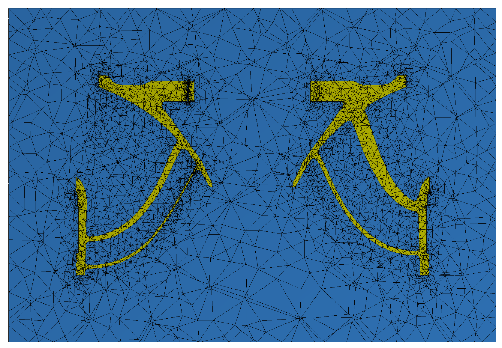
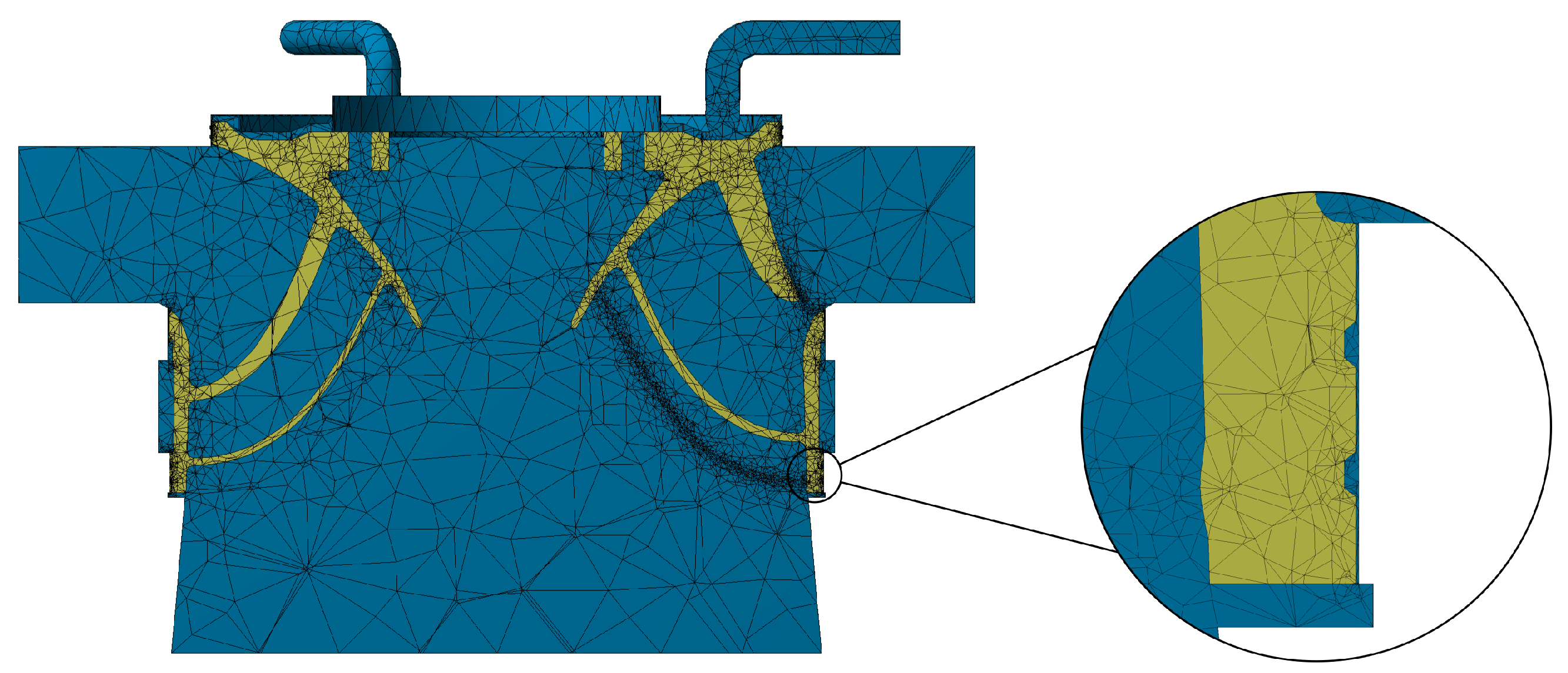
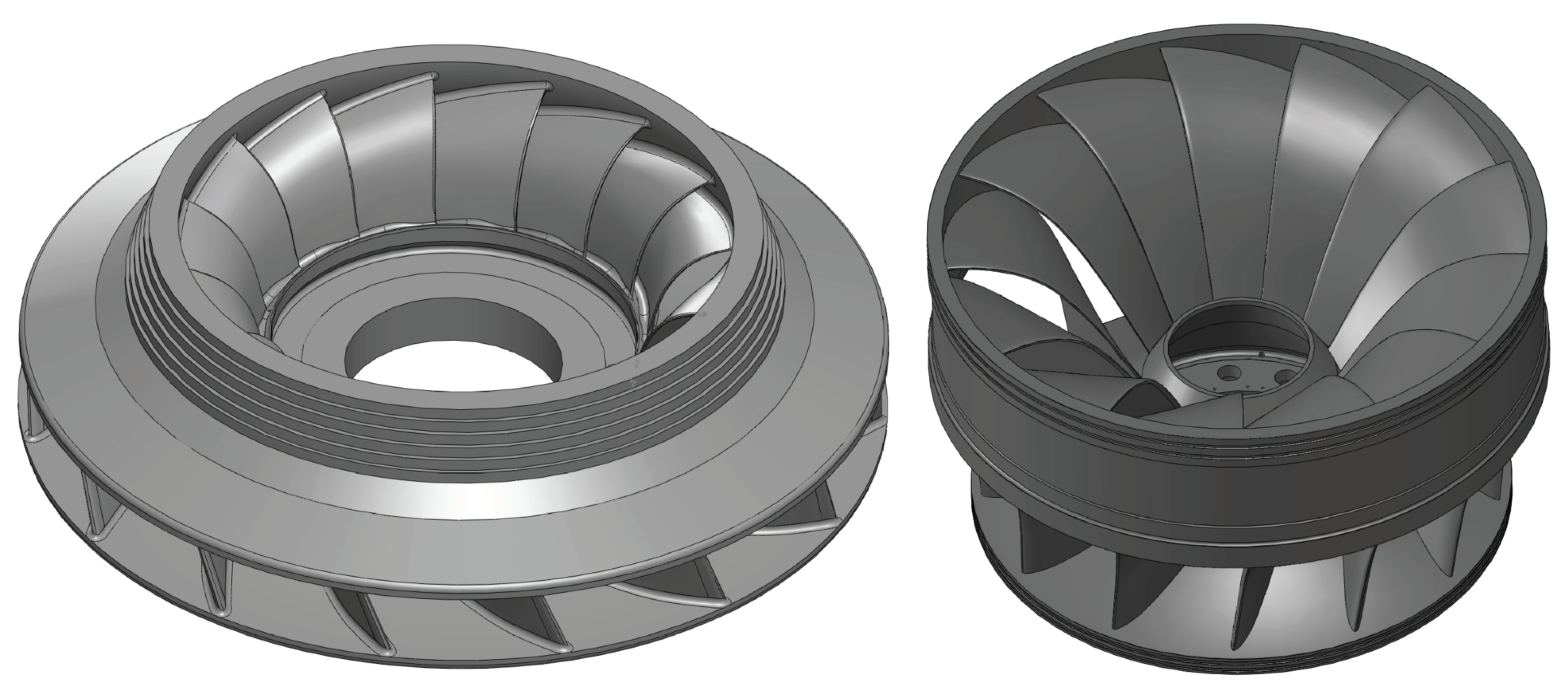
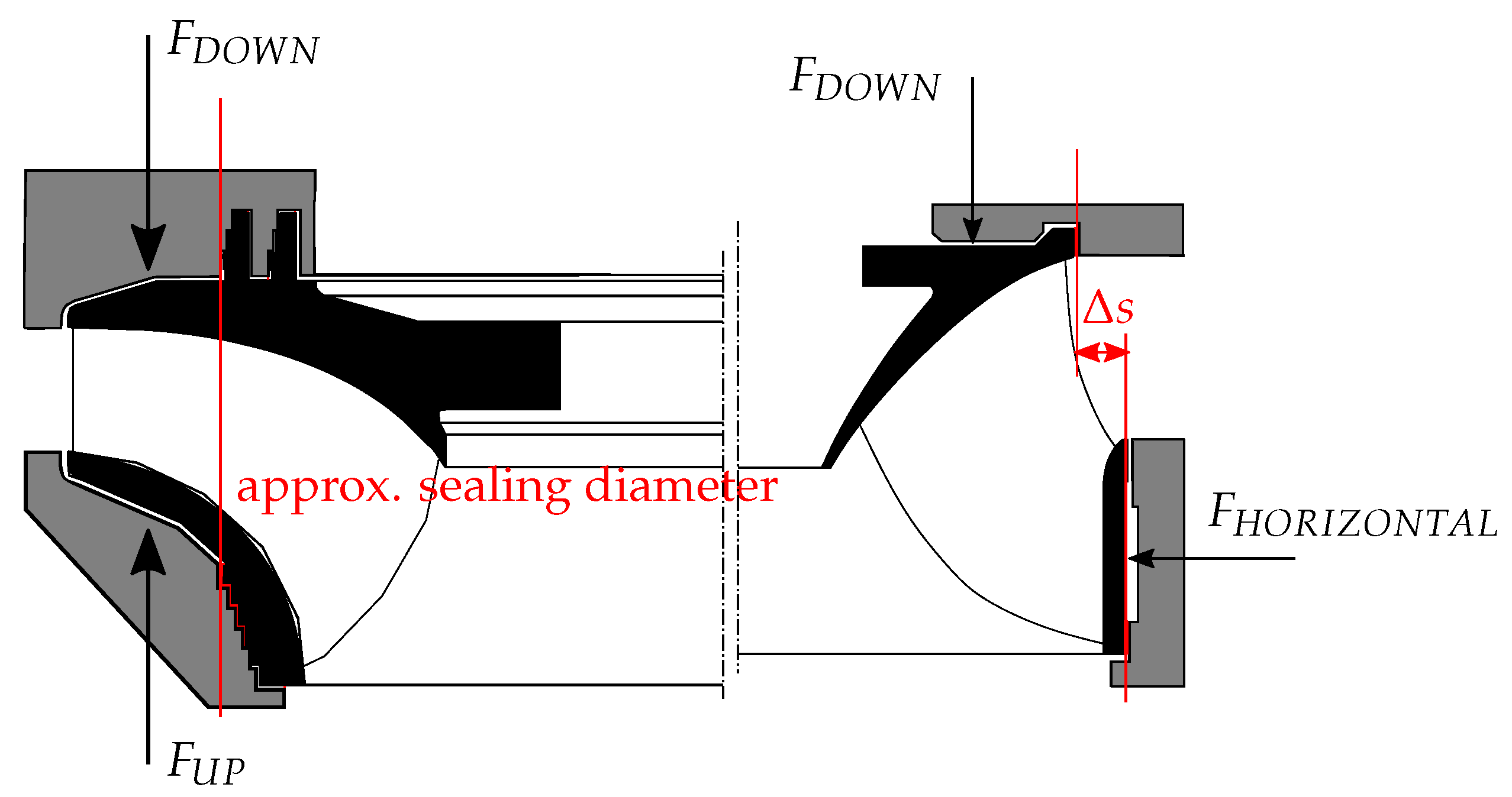
For the subsequent fatigue analysis, it is essential to apply the correct pressure distribution at the runner’s sidewall gaps. Since most of the pressure is released in the labyrinth seals, the turbine and sealing design has a considerable influence. Currently investigated turbine runners and their sealing positions within the runner sidewall gaps are shown in Figure 4 and Figure 5.

❸

Fixed support at bolt circle

The runner is fixed at the bolt circle towards the turbine shaft. Rotational as well as gravitational forces are taken into account. Optimization potential would be here the consideration of the screw connection or at least a circular ring approach in the size of the bolts diameter instead of using a circle. Such an approach would give a more rigid fixation then the circle one.

3.3.3. Investigated Operational Points

The FE analyses’ scope was investigating those operational points where the electrical grid synchronized machine was adapted to load changes. See also Section 3.1.4. The calculation of the mechanical stresses at the runner during the transient operating changes was too extensive in terms of simulation time and memory capacity.

The transient FE simulations follow the description of Section 4.2.2 of Paper I.

3.4. Lifetime Prediction

The lifetime prediction uses the damage accumulation hypothesis presented in Section 3.2.2 of Paper I. Utilizing the introduced transient assessment method offers the advantage of investigating all exciting frequencies of the occurring flow phenomena instead of single ones. Therefore the numerical method is equivalent to the measurement. The benefit is now the suspension in stress evaluation to the position of the strain gauges. Lifetime prediction is evaluated at the hotspots of the structure.

4. Results

The result section provides information about the CFD simulations, the modal analyses, FEA calculations, and lifetime prediction using numerical investigation. Before discussing the structural-mechanical results, a comparison of global integral CFD parameters versus prototype measurements provides information on the extent to which differences in the numerically calculated pressure fields already influence the results of the subsequent FEA computations. A comparison of prototype measurement versus numerical obtained values at these monitoring points follows. Pressure fields at the entire fluid domain build the base for further stress analyses. An additional step represents the determination of the natural frequencies.

4.1. Computational Fluid Dynamics (CFD)

4.1.1. Global Integral Parameters and Local Scalar Monitoring Points

To validate the transient flow calculation carried out in ANSYS CFX, a comparison of the global parameters head H, torque T, and efficiency $\eta$ with the measured values is used. For this purpose, the required variables are evaluated at two monitoring levels defined in the simulation model and at the turbine shaft and compared with the measured data at selected operating points (see Figure 22). The amount of the relative deviation between measurement (MES) and simulation (SIM) can be calculated via

$$\left|\delta \right|=|\frac{MES-SIM}{MES}|·100\%$$

(5)

Figure 22 shows the large deviations of global CFD parameters compared to measured ones among different operational points. These relatively significant differences can derive from unsuitable turbulence models combined with measurement uncertainties. As the flow at these deep part-load operating ranges is exceptionally chaotic, higher turbulence models are required resulting in more computing time. The depending problem of these results is an inadequate pressure field, consequently leading to wrong mechanical stress estimation at the investigated parts. Additional uncertainties also remain from coarse mesh discretization, for example. Higher turbulence needs, on special occasions, a local mesh refinement to determine the correct values. Not even the simulation time is turbulence-independent. A qualifiedly good answer needs some additional test runs and investigations—more information on that to come with Part IV of this paper series.

Another way to assess the numerical flow simulation’s general quality is to compare it with measured data at a monitoring point. This was achieved by defining a monitoring point in the numerical model at the location of the installed pressure sensor in the natural system and logging the scalar pressure variable. Comparing both scalar values gives an excellent impression of how close the numerical solution approximates reality.

Figure 23 shows a reasonable interpretation of the monitored pressure at the draft tube cone at the best efficiency point (BP) of the machine. There is still space for improvement at other operational points like part-load or low-load areas.

4.1.2. Pressure Distributions

The main objective of the numerical flow simulation is to calculate the transient pressure distributions and fluctuations in the fluid domain. For this purpose, it is necessary to calculate several runner revolutions transiently and export the resulting pressure distributions. They serve as transient boundary conditions within the framework of the FEA. The number of exported pressure fields depends on the time step size and number of revolutions of the computation. However, particular attention must be paid to calculating the pressure fields, as a deviation of the flow from reality inevitably results in an incorrect estimation of the mechanical stresses on the turbine runner.

4.2. Natural Frequencies of Investigated Parts

The subsection on natural frequencies contains the results of eigenfrequency and eigenmode simulations for the guide Vane, runner, and draft tube, as these components are essential for further investigations. The modal analyses of those components have been performed through numerical simulations by using the models described in Section 3.2. Subsequently, one has to clarify that there is no resonance situation within the power unit. A resonance situation would cause a severe safety problem and should be avoided. Resonance conditions appear if excitation frequency and eigenfrequency have the same value and damping of the system is low. Depending on the eigenmode of the component under these conditions cracks can be initiated and lead to a break down of the unit.

Following excitation frequencies have been determined and correlate to the range of appearance from the literature (see also Paper I for further information).

4.2.1. Guide Vane

Table 7. Eigenfrequencies of the guide vane and their modes.

Mode	Frequency		Mode
#	(Hz)		Illustration	Descrription
1	266			bending about x-axis
2	354			bending about y-axis
3	720			bending about x-axis
4	1159			torsion about z-axis
5	1191			bending about y-axis
6	1256			bending about x-axis
7	1698			torsion about z-axis
8	2026			bending about x-axis

shows the results of the numerical modal analysis of the free-swinging guide vane in air. The orientation of the coordinate axes is shown in Figure 8. The first natural frequency of the guide vane in the air is at 266 $\mathrm{Hz}$, the next possible excitation frequency would be the frequency of the vortex shedding at 232 $\mathrm{Hz}$. The first natural frequency of the assembled guide vane (torsion mode) is even higher at 333 $\mathrm{Hz}$.

4.2.2. Runner

The following

Table 8. Eigenfrequencies of the runner and their modes.

Mode	Runner in Air (Model 1)	Cylinder Model (Model 2)		Runner Sidewall Gap Model (Model 3)
	Frequency (Hz)	Frequency (Hz)	Deviation	Frequency (Hz)	Deviation
torsion	130	117	−10%	109	−16%
tilting	171	140	−18%	70	−59%
ND2	177	133	−25%	82	−54%
ND3	258	161	−38%	136	−47%
ND4	321	169	−47%	171	−47%
blades	328	218	−34%	253	−23%

shows the natural frequencies and eigenmodes for the runner. Six different modes have been investigated and it is remarkable that the runner in air shows huge deviations related to the runner in water investigation. Out of this observation the added mass effect seems to be quite large for prototype investigations.

4.2.3. Draft Tube

• Draft tube eigenfrequency and mode
  The following table shows the measured eigenfrequencies versus the calculated ones.
  Taking water volume and attached concrete of the draft tube into account the deviations are rather low.
• Resonance with runner
  Considering the excitation frequencies of

  Table 9. Excitation frequencies.

  Cause	Acronym	1. & 2. Frequency
  Rotation	$F_R$	7.14 Hz
  Draft tube vortex	$F_{DTV}$	1.4 Hz and 5.7 Hz
  Generator	$F_{GEN}$	50 Hz + harmonics
  Gate passing	$F_{RSI}$	185 Hz
  Vortex Shedding	$F_{VOS}$	232 Hz + harmonics

  and correlating them with the results of

  Table 10. Draft tube eigenfrequencies.

  Measured (in Hz)	Calculated (in Hz)	Deviation (in %)
  232	232.04	+0.017%
  464	461.54	−0.530%
  464	465.53	+0.329%
  594	593.87	−0.022%
  695	695.90	+0.129%
  927	927.22	+0.024%

  one notices a resonance problem caused by vortex shedding of the runner. This investigation has been published by [35].

4.3. Mechanical Stresses at the Runner by Means of FEA

The position and the value of the highest occurring stress at the runner depend on the respective considered operating point of the plant. In [35,40,42] it has already been shown that the highest dynamic stresses are expected near the positions of R1 and S2 in the partial load range at $P/P_{RP}=44\%$. However, the simulations aimed not only to find the critical operating point but also to numerically investigate the plant’s entire operating range concerning occurring stress conditions and damage effects on the runner structure. In the following results, a fundamental distinction must be made between stresses on the defined strain gauge surfaces for model validation and the maximum principal normal stresses occurring at the respective operating point.

4.3.1. Stresses at Strain Gauge Places

For stress evaluation on the strain gauges, the averaged value of the nodal points lying on the strain gauge carrier foil surfaces is used. The positions on the runner surface and the corresponding designation of the strain gauges can be found in PART III of this publication series, and partly at [42]. For the strain gauges S1–S6 and D1–D6, the averaged normal stress is used. For rosette R1, the first and second principal normal stress is evaluated. The results are related to the yield strength ${\sigma }_y$ of the runner material and plotted in % of the rated power $P_{RP}$.

Static Stress Results

The Figure 24 and Figure 25 show the static mean stress ${\sigma }_m$, defined as the arithmetic mean value of the discrete simulation signal at the suction and pressure side transitions to hub and shroud.

It is noticed that the static stresses at the transition from runner blade to hub are significantly higher than at the shroud. Stress values on the pressure side show a clear dependence on the respective operating point. The maximum occurs at R1 in case of overload. For S2, the highest stress with almost constant value results at the suction side.

Dynamic Stress Results

To compare the dynamic stress components, the RMS value of the time signal is used and shown in Figure 26 and Figure 27.

The dynamic results show that the critical operating point in terms of fatigue is between 16 and 19 MW at the transition from blade to hub, which is also mentioned in [35,40,42]. It can be considered that the most intense transient flow effects in the CFD simulation occur in this partial load range and thus cause the highest dynamic stress components in the FE simulation. The dynamic stresses are lowest near the design point of the plant. The absolute values at the hub are higher, which indicates partial load turbulences and vortex ropes. The low dynamic stresses at the runner inlet, on the other hand, suggest a low influence of the RSI.

4.3.2. Stresses at Hotspots (Change of Hotspot)

The FE results show that the point on the runner with the highest occurring principal normal stress varies depending on the operating point and does not necessarily coincide with one of the defined strain gauge positions. Therefore the definition of the so-called stress hotspot (HS) was introduced.

As shown in Figure 28, the hotspot for all operating points is located near the trailing edge, in the transition radius from the runner blade to the hub. For the operating points $P/P_{RP}=$ 7–37%, the hot spot is located on the suction side near the strain gauge S2 and changes for $P/P_{RP}=$ 44–105% to the pressure side of the runner blade close to the rosette R1. This behavior requires the definition of two critical failure points on the runner. One is hotspot 1 (HS1), located on the blade’s pressure side close to rosette R1, and the other is hotspot 2 (HS2), located on the suction side close to strain gauge S2.

Static and Dynamic Stress Results

Due to the proximity to R1 and S2, similar behavior is observed for the hotspots. Furthermore, the change of the highest principal normal stress position at $P/P_{RP}=44\%$ is clearly visible in the diagram on the left side of Figure 29. The maximum occurring amplitude is at HS1 for $P/P_{RP}=105\%$ and is significantly higher than for HS2 at the same operating point. Near the optimum and the rated point, however, there are hardly any differences.

4.4. Damage Factors without Correction

The modified linear damage accumulation hypothesis “Miner Elementar”, according to Palmgren and Miner [48], is used to determine the damage factors numerically. The load spectrum obtained from the stress curves by means of RFC is compared to the SN-curve of the runner material in water [49]. The S–N-curve was specified in as test report for the runner material X5CrNi13-4 in water by the Fraunhofer Institute for Structural Durability and System Reliability (LBF). In preparation for the Rainflow-Counting algorithm, the stress curves were filtered by peak through detection and then extrapolated using statistical extreme value theory [50]. The mean stress on the amplitude is considered by the Haigh diagram and the mean stress sensitivity. This procedure has already been applied to determine a Francis turbine’s load spectrum in former publications [41].

4.4.1. Damage Factors at Strain Gauge Places

Figure 30 shows the damage factors D for the two strain gauges R1 and S2 near the hotspots over the plant’s entire operating range. The values refer to a continuous operating time of 1 year at the respective operating point.

As expected, the operating points for $P/P_{RP}$ = 37–44% are particularly damaging to the runner for both strain gauges, with the value for R1 being slightly higher. For both strain gauges, the minimum occurs at the rated point. Furthermore, it can be seen that the low partial load at S2 has a more substantial effect, whereas in the range of $P/P_{RP}$ = 51–100% higher values at R1 result.

4.4.2. Damage Factors @ Hotspots

The damage factors for the two stress hotspots HS1 and HS2, shown in Figure 31, are derived analogously to the above explanations.

Figure 31 also shows that the operating point with the most severe damage is at $P/P_{RP}=37\%$ and operation close to the rated point or optimum will have a significantly less damaging effect on the runner structure. In general, one can conclude that the numerically determined damage factors on HS1 are higher on average.

4.5. Numerical Lifetime Prediction (without Validation)

To formulate statements regarding the fatigue strength and the associated lifetime of a Francis runner, calculated damage factors as shown above are not sufficient. Qualified statements require knowledge of the load spectrum of the power plant. For this purpose, the two load scenarios’ operating times—base load and grid control—shown in PART I, Section 1.2.3, Figure 5 were used. With this operating times distribution and the previously determined damage factors, the numerically predicted lifetime can be estimated.

Hotspot Investigation

The calculated values for the critical points HS1 and HS2 of the two scenarios—base load and grid stabilization—are shown in

Table 11. Expected lifetime for critical hotspots HS1 and HS2 in years for scenarios base load and grid stabilization.

Position	Base Load [Years]	Grid Stabilization [Years]
HS1	13,517	363
R1	35,969	653
HS2	22,676	472
S2	70,265	1309

. Looking at the lifetime determined from the simulations, hotspot HS1 on the pressure side at the transition from runner blade to hub turns out to be the critical failure point for both load scenarios. However, it should be mentioned that this results in unexpectedly high values of lifetime, especially for base load.

Such long lifetimes cannot be correct. It needs further failure investigations of the entire procedure to determine the main influencing parameters of such a numerical assessment. Part III shows the measured data results knowing that those results are only valid for the places where the strain gauges are placed. The problem is that measured data give the allowable stresses but not at the exact places where the maximum stresses appear. To place a strain gauge strictly at the hotspot is impossible. Significantly if the hotspot changes over the operational points, only a numerical investigation can solve this problem if the stresses are determined correctly. To close this gap, a validation based on prototype measurements, respectively, a calibration of the obtained results is necessary. Detailed knowledge of uncertainty parameters is needed to obtain proper calibration factors. Most influencing parameters must be identified, and sensibility to those parameters has to be given. Part IV handles those sensitivity problems and numerical results, shifting to correct evident values.

5. Conclusions

The structure of the assessment model and the general procedure for determining the stress condition and the runner’s damage factors are conclusive. They have already been applied successfully for individual operating points in several investigations. With this methodology, it is quite possible to estimate the failure-critical point within the runner structure and to assess the individual operating areas concerning damage. However, for accurate and reliable lifetime values, further investigations are necessary, starting with CFD modeling and ending up with the methodology for calculating the damage factors. More complex multi-axial approaches, strain-based, critical plane, or even fracture mechanics models are future work goals.