Low-Cost Sensors for Indoor PV Energy Harvesting Estimation Based on Machine Learning

Abstract

With the number of communicating sensors linked to the Internet of Things (IoT) ecosystem increasing dramatically, well-designed indoor light energy harvesting solutions are needed. A first step in this direction would be to be able to accurately estimate the harvestable energy in a specific light environment. However, inside, this energy varies in spectral composition and intensity, depending on the emission source as well as the time of day. These challenging conditions mean that it has become necessary to obtain accurate information about these variations and determine their impact on energy recovery performance. In this context, this manuscript presented a method to apply an innovative energy harvesting estimation method to obtain practical and accurate insight for the design of energy harvesting systems in indoor environments. It used a very low-cost device to obtain spectral information and fed it to supervised machine learning classification methods to recognize light sources. From the recognized light source, a model developed for flexible GaAs solar cells was able to estimate the harvestable energy. To validate this method in real indoor conditions, the estimates were compared to the energy harvested by an energy harvesting prototype. The mean absolute error percentage between estimates and the experimental measurements was less than 5% after more than 2 weeks of observation. This demonstrated the potential of this low-cost estimation system to obtain reliable information to design energetically autonomous devices.

1. Introduction

The development of the Internet of Things (IoT)- or Wireless Sensor Networks (WSNs)- based applications is growing significantly. Reaching energetic autonomy for the associated sensors remains a challenge, however. On one hand, a lot has been done to reduce their power consumption. On the other hand, a growing community of researchers has been working on improving the technologies to harvest enough power from the nearby environment to supply electrical energy to such devices [1,2]. One of the most common means to achieve such energy recovery is photo-electrical conversion, based on photovoltaic technologies. For decades, databases and software have been used to accurately estimate the energy that can be harvested outdoors from square meters of sun light, anywhere on earth [3]. However, under indoor light conditions, no standards have yet been created. Indoor light is usually composed of several different light sources (artificial and natural, direct and reflection). Therefore, characterization, standardization, and generalizations are more challenging in such environments as compared to outdoor light environments. That lack of standard made the task of establishing the level of energy harvestable in those indoor conditions much more complex.

Nevertheless, many studies have been conducted to address this issue. Some have proposed investigation of the influence of light source spectra on harvesting efficiency [4,5,6,7,8,9]. These methods were aimed toward better design dimensions of energy harvesters according to the needs of the device, in order to make them energetically autonomous. Mostly artificial light sources, are considered in models [10,11] even though natural light can be a significant indoor light source [12] and studies focusing on PV performances in low light conditions [1,4,13,14,15,16,17]. To go a step forward, we believed it necessary to estimate the real harvestable amount of electrical energy, as in the reference [18], to give more practical insights into harvesting system design—with consideration given to the specificity of the PV converters and the spectral composition of light sources. The real harvestable amount of energy, in this sense, refers to the need to consider losses in unideal solar cell converters coupled to an unideal power management integrated circuit (PMIC) and unideal batteries. The efficiency of all these elements that compose the harvesting system must be evaluated to obtain accurate estimates. Determining the amount of real light requires consideration of both artificial and natural light sources, including reflections and scatterings. Long periods must also be investigated because of daily and seasonal light variations. Considering that these have been undertaken in a study recently published by Politi et al. [19] in which a spectrometer was used for several weeks to quantify the harvestable energy in a specific location. Estimation results were compared to measurements of the energy harvested by a prototype into the LiPo battery of a real electronic device. After several days, the experiment has shown a very good match between estimates and practical measurements, demonstrating the potential of this method to help in the design process of IoT energy harvesting systems. However, the main drawback of this technique is the price of a spectrometer and its need for calibration and recalibration, which implies limitations to the number of days this method can be utilized without any maintenance and surveillance.

In this methodological paper, we pursued the implementation of an innovative approach to achieve good performances on the estimation of practical energy harvestable in real indoor environments. Figure 1 shows the building blocks of our complete system, which is detailed in the experimental setup section. This method was first presented by Sarik et al. [5], showing that light source recognition can be achieved with low-cost sensors. In the continuity of this work, Ma et al. [17] were able to confirm these results and demonstrate the potential of machine-learning classification methods. Based on those results, it was possible to use that method of light classification in association with models of PV converters to approximate power generation. Ma et al. more recently showed convincing experimental results [20]. Here, a complete system was developed using low-cost devices combined with a model implemented in the report mentioned [19]. The aim of this paper is to demonstrate the possibility of using the power estimation method and system in real-world conditions (mix of natural/artificial light sources). This study also benefits from the development of an energy harvesting system. Comparing the presented method estimates to the energy harvested by this prototype, it is possible to confirm the validity of this method. In the following sections, we described how we empirically chose the best classifier for our application. Energy harvesting estimation results we have obtained in real indoor light conditions are presented as well.

2. Experimental Setup

2.1. Low-Cost Analysis Device

The main challenge regarding the method described in this article was to replace the expensive spectrometer described in Politi et al. with a low-cost low-tech system which can be widely deployed in the building to be tested. This system is composed of two sensors, widely available on a commercial basis and costing a few dollars each:

• The first sensor, the TSL2561 from TAOS [19], is based on two photodiodes: (i) the first one is a broadband (BB) photodiode, sensible to the whole visible + near infrared 300 nm to 1100 nm wavelengths, returning a digital BB value and (ii) the second one is a narrower near infrared (IR) photodiode, sensible from 500 nm to 1100 nm wavelengths, returning a digital IR value. From these two photodiodes, an ambient light level value in lux could be derived using an empirical formula to approximate the human eye response. This value is returned as the digital LUX value.
• The second sensor, the ISL29125 from RENESAS [20], uses a matrix of three photodiodes, each sensible to different parts of the visible spectrum: blue, green and red. It provides a set of three digital values R, G, and B.

A low-cost low-power ESP32 microcontroller from ESPRESSIF, able to communicate through WiFi, is used. Its purpose is to gather, treat and send the data via wireless communication protocols to a database which was stored in our server. This microcontroller was mounted on the commercially available HUZZAH32 board (Adafruit), which integrated a USB connector used for battery charge and serial communication. An additional PCB is designed as a motherboard to connect the two sensors to the ESP32 board, resulting in a compact device, as small as 35 cm³, as shown in Figure 2a,b.

This device is able to acquire what we call “pseudo-spectra”, which could be assimilated as very low-definition spectra. Even if the level of information provided by pseudo-spectra was low, it remained sufficient to observe variations, depending on the light source, as can be seen in Figure 2c. If deemed necessary, pseudo-spectrum acquisition can be done (via USB or WiFi) at a relatively high rate (few measures per second).

2.2. Classification and Training

From the low-resolution experimental pseudo-spectra provided by the low-cost device, machine learning algorithms are used to classify the different possible light sources. The method chosen for that purpose, called supervised machine learning classification, is a classical Artificial Intelligence (AI) machine learning method. This method is implemented through the Classification Learner App made available by MATLAB in its Statistics and Machine Learning toolbox. In our study, we have divided the light sources into 7 classes: LED 3000K, LED 4000K, CFL 2700K, CFL 6500K, natural scattered light from a clean sky through a window, natural scattered light from a cloudy sky through a window and, finally, mere darkness. Varying the light intensity of each class, under controlled lab conditions, we built a dataset of 126 different pseudo-spectra. Classification training is based on this dataset. For each measurement of each different light source, the tested light class is manually input to the dataset. Several classical classifiers included in the Classification Learner app have been simultaneously trained.

Table 1. List of the 24 algorithms tested as classification methods in this paper. These algorithms are the most classical ones used in supervised machine learning for multinomial classification included in the Classification Learner app found in the Statistics and Machine Learning toolbox.

Tree	Discriminant	Naive Bayes	Support Vector Machine (SVM)	K-Nearest Neighbor (KNN)	Ensembles
Fine	Linear	Gaussian	Linear	Fine	Boosted Trees
Medium	Quadratic	Kernal	Quadratic	Medium	Bagged Trees
Coarse			Cubic	Coarse	Subspace Discrimination
			Fine Gaussian	Cubic	Subspace KNN
			Medium Gaussian	Cosine	RUSBoosted Trees
			Coarse Gaussian	Weighted

lists 24 classical algorithms used in supervised machine learning for multinomial classification. The main types of classification methods were the Decision Trees, the Discriminant Analysis, the Naïve Bayes, the Support Vector Machine (SVM) Classification, the K-Nearest Neighbors (KNN) and finally Classification Ensembles. These algorithms learn to classify data from training samples whose classes are known.

Thanks to the dataset of the 126 pseudo-spectra, each associated with one of the 7 defined classes, the training of the 24 classifiers is possible. It allows the building of the trained classifiers seen in the data section of Figure 1. One of the challenges is to have classifiers reliable enough to be able to properly classify new unknown pseudo-spectra.

2.3. Spectral Reconstruction and Calculation of the Harvestable Energy

The spectrum database seen in the data block of Figure 1 was recorded, thanks to a commercial calibrated spectroradiometer, the StellarRAD from StellarNet Inc., equipped with a CR2 cosine receptor with a wavelength range from 350 nm to 1100 nm. The high resolution 7 spectra of the database, corresponding to the 7 classes used in our study, were necessary for the reconstruction stage of one reliable, trained classifier, given its classification results in new light environment observations. Then, depending on the class found by the proper classifier and the LUX value to tune the intensity properly, a high-resolution spectrum could be reconstructed.

Finally, to estimate the harvestable light energy in the surroundings of the low-cost sensor, we used a model, published in a previous article [19], that takes the reconstructed spectra as input instead of bare high-definition spectra from an expensive spectrometer. This model is based on a one-diode photovoltaic model using the measured external quantum efficiency (EQE) and the saturation current density–voltage characteristic measured in darkness (J-V_dark). Both are unchanging intrinsic values and only depend on the PV converter technology considered. These EQE and J-V_dark characteristics are contained in a database called Spectral Response and Dark Current Density, as seen in the data block of Figure 1. The spectral response was measured with a custom-built setup composed of a Xenon lamp, a monochromator equipped with two diffraction gratings, a filter wheel to remove the higher diffraction orders of radiation, and a lock-in amplifier. These measurements were calibrated with Si and Ge photodiodes (Thorlabs FDS100-CAL and FDG03-CAL, respectively) to cover the whole wavelength range of interest. The dark current density–voltage curves J-V_dark of the different technologies of PV converters were collected by the SMU 2450 from Keithley.

2.4. Instrumented Prototype: Energy Harvester

To evaluate the accuracy of the method presented below, it is necessary to compare the energy harvesting calculation results with experimental measurements of the energy harvested by real energy harvesting systems. To perform such measurements, an instrumented energy harvesting prototype is created, based on 2 GaAs solar cells. It integrates power measurement units (INA219 from Texas Instrument Inc., Dallas, TX, USA) suitable for monitoring the power harvested from solar cells by a power management integrated circuit (PMIC AEM10941 produced by ePEAS), then stored into a battery. The picture shown in Figure 3 display this equipment and the data recovery system attached to it. In the same way as the low-cost light analysis tool, this system gathers data with a microcontroller that transfers its measurements to another microcontroller. This other microcontroller is in charge of the data transmission to our server database. Then, accessing this database, it is possible to analyze these data to compare them to the results of our low-cost method, as seen in Figure 1.

3. Classification of Light Sources

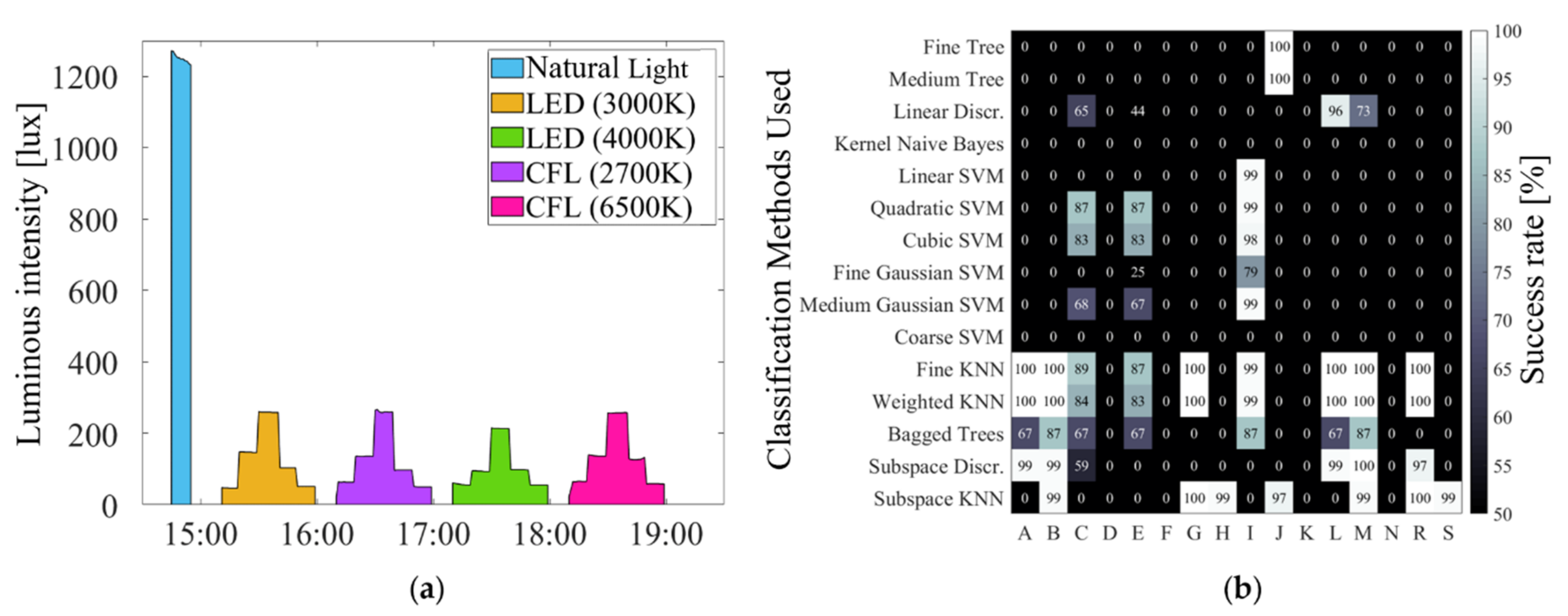
3.1. Classification Methods Training Performances on Raw Data

Thanks to the Statistics and Machine Learning toolbox from MATLAB and its Classification Learner app, classifiers can be trained very quickly. Those trainings can be performed with all six values of the pseudo-spectra or with a reduced number of them. In our study, we chose the 11 configurations seen at the bottom of Figure 4. For example, configuration A relied on all values from the sensors, while configuration I utilized only the R and IR values from the sensors. Combining each of the 24 classification methods with each of these 11 configurations resulted in 264 classifiers to train. Those trainings starts with the 126 pseudo-spectra observed and each classifier used a 5-fold cross validation. The cross-validation process consists of separating the dataset randomly into five folds. Four of them are then used to train the classifier. Once the training completed, the classification capability of the classifier is tested on the remaining fold. This process is reproduced to obtain five iterations where each fold is used as the test fold. Finally, the overall performance of the classifier is found by calculating the mean success rate of the five classification tests. Results of that process are shown in Figure 4 for the classifiers and configuration described previously.

A first observation is that none of the 264 classifiers reached a total 100% of classification success. A second look at the results showed that some classifiers seemed more adapted to our application: Cubic SVM, Fine KNN or Weighted KNN. We noted that the configurations with only 2 or 3 features of the dataset performed almost as well as configurations with 5 or all data features. Finally, we conclude that, with this dataset, the best classifier is the Cubic SVM for the configuration A, which obtained 96.8% of correct classification. It can correctly classify 122 observations over 126.

To understand errors produced by the trained classifiers, a decision surface of each of them can be plotted. Indeed, each classification method used a different algorithm to establish the boundaries that separated the observations of different light sources. Once trained, each classifier used its algorithm to determine the parameters of the equations that defined these boundaries. Decision surfaces help visualize the limits established between classes by classification method. As an example, Figure 5a displays the 126 data represented in a space corresponding to the IR versus R ratio. Figure 5b,c illustrates the decision surface of the Cubic SVM and Fine KNN classification method in configuration I (for an easy representation in 2D space). Let us note that, for the configuration with more than 3 data, the representation of surface decision would have been more complex. In practice, good classification success rates were more likely to be obtained when values of the classes were distinctively separated from each other. However, in this particular case, some very narrow zones are visible and with experimental dots right at the boundaries it induces errors of classification. It can explain the numbers from Figure 4, that Cubic SVM Configuration I had a rate of success of 86.5% while the Fine KNN Configuration I had a rate of success of 88.1%. More decision surfaces from different classification methods can be found in Figure S1 in the Supporting Information. Further research on the particularities of each classification method will be needed to better understand their classification performance in our use case. However, the field of supervised machine learning was beyond our scope of study and would require further investigation on its own.

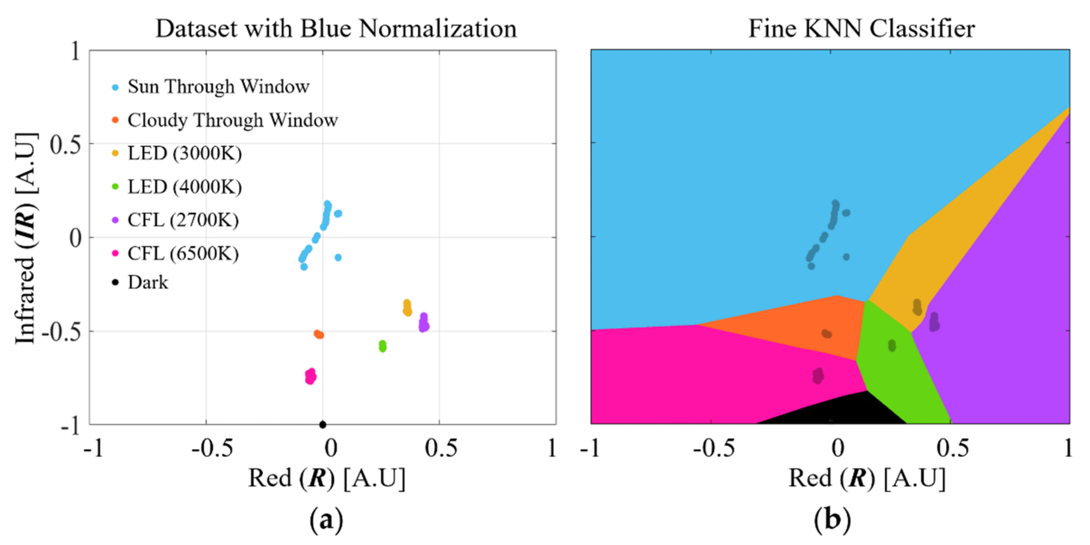
3.2. Normalization Impact on Classification Performances

Because the light source classes are not concentrated in zones distinct from each other but distributed in intensity over all their features, it is complex for classifiers to achieve successful light source classification. The poor results obtained during training suggest an underfitting for the dataset used. Although underfitting can be attributed to the small sample size of our dataset, unlike natural light sources, artificial light emissions tended to remain constant once turned on. Consequently, a high number of samples for artificial light should not be necessary.

However, for natural light sources, the problem of the number of observations necessary to cover their intensity range remains. One way to get around this problem is to eliminate the intensity variation for the classifiers training. Applying a difference normalization to the data, it is possible to constrain the fluctuation of the data to spectral variations only. This method of normalization is commonly used in fields of remote sensing using multispectral or hyperspectral data. For instance, it can help to distinguish vegetation health with the Normalization Difference Vegetal Index (NDVI) [21]. This method is based on a simple calculation between two values: dividing the difference of the two values by their sum, as shown in Equation (1).

$$\mathit{\text{Normalized Difference Data}}=\frac{\mathit{\text{Data to Normalize}}-\mathit{\text{Normative Data}}}{\left(\mathit{\text{Data to Normalize}}+\mathit{\text{Normative Data}}\right)}.$$

(1)

As an example, Figure 6a displays the 126 data normalized to B value. Applying this method, to each measurement, a clearer map of the light source classes emerged (Figure 6b), which is the decision surface created using the dataset normalized by B with the Fine KNN classification method in configuration I. With this figure, significant improvement in the way classes could be recognized can be noted. The decision surfaces are better defined and able to allow better classification results. As a matter of fact, the classification training with the Fine KNN configuration I algorithm reached a perfect score of 100%.

Tests were conducted for all the 264 configurations to establish the impact of the blue normalization (B) of the differences. As visible in Figure 6b, for a Fine KNN classifier with B normalization, classifiers trained on normalized datasets were fed with classes distinctively grouped and no longer spread out according to their intensity. More decision surfaces from different classification algorithms trained for different normalization values can be found in Supplementary Figure S2. Figure 7 summarizes the scores for all the 24 classification methods with configuration from A to K configurations, tested with B normalization. A clear improvement of the success rates in almost all the configurations can be observed. It has to be noted that the K configuration gave no result. Because its input is reduced to only one datum, IR, leading to poor performances, such classifier is not trained.

One detail about normalizing by difference is that, if the normalization is also applied to the value chosen as the norm, it will be normalized by itself and inevitably equal to zero. To evaluate the effect of these 0 values on classification, additional configurations are tested. These configurations are almost similar to the 11 initial configurations (A to H), but exclude the data used for normalization. Details on the configurations for each normalization are available in supporting Figure S3. Finally, only 8 configurations are added (from L to S). As an example, Figure 5 shows, the different configurations used for the B normalization and the results provided by the 5-fold cross validation. In this case, three configurations out of the 19 are not tested: I configuration would only have had IR values, and in the case of N and P configurations, they would have been similar to C and E configurations, respectively. In total, for the B normalization, 384 classifiers are tested, many of them reaching performances over 90%. A total of 40 of them achieved a 100% success rate, mainly with the Fine and Weighted KNN methods.

Similar tests are done with the other colored normalizations. As shown in the complementary information, the number of classifiers to be tested is the same for the green (G) and red (R) normalization (384), and a bit less for the BB and IR normalizations (336 and 264, respectively). A total of 1752 classifiers are trained. Results of their 5-fold cross-validation performances are shown in the Supplementary Materials. Of these 1752 classifiers, 267 achieved 100% correct classification, a significant improvement compared to classification performances without normalization. Figure 8 summarizes, in one table, the number of classifications with 100% success, depending on the classification method applied and the feature configuration used, all normalization combined. It appears from this figure that, in this training phase, Fine KNN and Weighted KNN are the most performant classification methods, as well as the L configuration seems the most appropriate feature configuration.

3.3. Successfully Trained Classifiers in Confrontation to New Controlled Pseudo-Spectra

In the next step, the 256 best classifiers are confronted with new observations from the compact low-cost device. These observations are made in a controlled light environment consisting of several single light sources, for which classifiers were trained: LED 3000K, LED 4000K, CFL 2700K, CFL 6500K and cloudy sky behind a window at different light intensities, as seen in Figure 9a. After analysis, the accumulated data from the compact device are provided to the classifiers to obtain their classification results. Even if trained in similar conditions, classifiers can have very different success rate, mainly because of the overfitting effect. This means that the classifier is overfitted to the training data given and not able to correctly recognize data that are not very similar to that. Such classifier is therefore not able to generalize its classification method to other data that were similar but not identical to those used for its training. The results obtained on the new controlled environment are shown in Figure 9b. Note that the columns from configurations O, P and Q are removed as no classifier was able to reach the score of 100% after the 5-fold cross validation process. For the same reason, unreliable classification methods were also removed, like Coarse Tree, Quadratic Discriminant, Gaussian Naïve Bayes, some KNN (Medium, Coarse, Cosine and Cubic), Boosted Tree and, finally, the RUSBoosted Tree.

The main result of this experiment, shown in Figure 9b, is that more than half of the classifiers that reached 100% correct classifications in training had 99% success recognizing the new spectra. 42 classifiers reached 100% correct classification, mainly from the G and B normalizations. Classification results for all normalization are grouped in supporting Figure S4.

3.4. Trained Classifiers Performances on Pseudo-Spectra from Uncontrolled Light Environment

To go further on testing the 42 classifiers that successfully classified light sources in controlled conditions, it is necessary to evaluate their performance in real uncontrolled indoor conditions. In such conditions, light is usually a mix of artificial and natural sources. The problem this raises is that the nature of a real light environment is richer in spectrum and intensity variations in the real environment tested than the reduced environmental data used for training and generalization of classifiers. This makes the comparison of performance between each classifier more delicate than in the previous steps.

The method chosen to evaluate the performance of the classifiers is based on two criteria. On the one hand, a classifier is considered valid if, as in the previous steps, it correctly recognized a light source when it is the only source present in the environment. On the other hand, when the light environment is a mix of several sources, the classifiers are evaluated on their ability to distinguish which source of radiation is the main contributor in terms of irradiance. In other words, a light source needs to be recognized as the main light source when it radiates more than half of the irradiance measured in the environment. For example, during the day, natural light is usually predominant, compared to artificial light. On that criterion, a classifier is considered performant if the main source switched from natural light to artificial light as soon as daylight decreased below 50% of the total power radiated. For this experiment, tests were conducted an indoor environment globally composed of two types of light sources: a LED 3000K and a window facing south-east with a clear blue sky. For several days of tests, the LED 3000K, constant untunable lighting, was left on during the entire working day, making it easier to observe the switching ratio.

After several days of experimentation, results show that only 23 classifiers over the 42 tested could distinguish the different classes properly observed in the real indoor environment: LED 3000K, blue sky through a window and dark. During these tests, a precise measurement of the irradiance was carried out with a compact spectrometer. This measurement enables the calculation, at each moment of the day, of the percentage of the total incident radiation emitted by the artificial LED 3000K and by the natural light through a window. As a result, when a classifier switches from a recognized source to another, the ratio of natural light versus artificial light can be determined. As per a criterion established earlier, the more this switching point occurs near 50%, the more the classifier tested is considered reliable.

Figure 10 shows the classification results of a typical day, for the two best classifiers using the Fine KNN method with the blue normalization using the G and R configurations. On average, over different days, these classifiers were able to switch consistently from one source to the other with switching ratios around 45%. This means that if the irradiance emitted by the LED in the environment is larger than 45% of the total irradiance, the classifier recognize this source as the main one. Otherwise, the classifier determines that the environment is composed of natural light through a window. The average switching ratio of all the other classifiers is shown in the Supplementary Figure S5. From these results, K-nearest neighbor (KNN) methods of classification seems appropriate to our application in combination R or B normalization.

4. Harvestable Energy Calculation

A proper calculation of the harvestable energy in specific locations required pseudo-spectra to be classified correctly. Then, from the class recognized, a full spectrum could be reconstructed to meet the resolution of a spectrum acquired by a spectrometer. This reconstruction process relies on two different data: reference spectra acquired by a compact spectrometer and the light intensity (LUX) data acquired by our low-cost sensor device. First, the intensity of the spectrum must be tuned such that its illuminance (irradiance weighted according to the photopic luminous efficiency function) corresponds to the LUX value. Then, the harvestable energy is estimated, as described in Politi 2021. The light source classification method used in the following section is one of the most efficient seen in the previous chapter: the Fine KNN with B normalization and associated with configuration R.

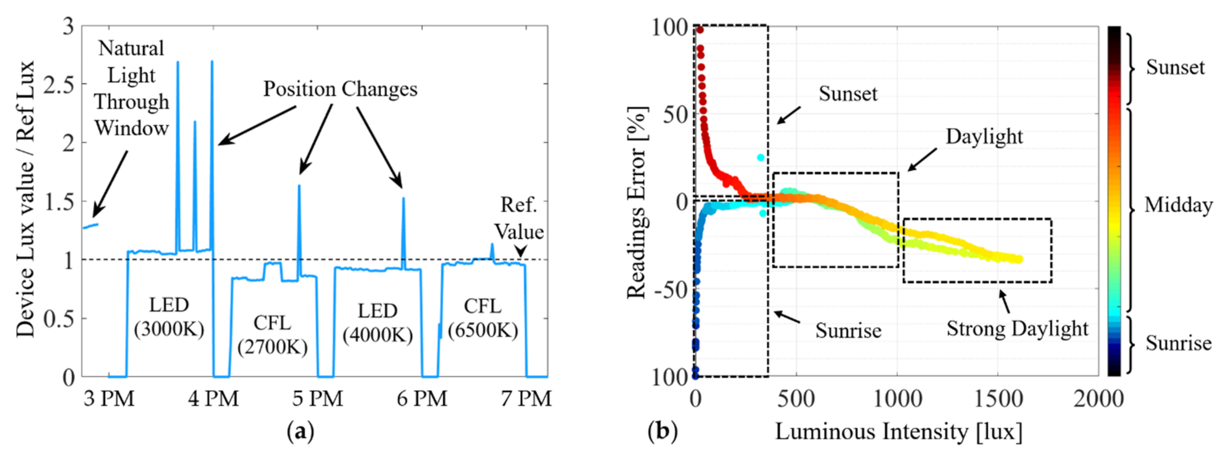
4.1. Sources of Error for Spectra Reconstruction

As stated previously, a good spectrum reconstruction needs a reliable value of light intensity. For this, the data LUX from the low-cost TSL2561 sensor is used. But comparing the lux value from this sensor to the reference lux calculated from an expensive calibrated spectrophotometer, a difference as important as 30% can be measured, as seen in Figure 10a. Depending on the class of light recognized, a correction factor must be applied to the lux data obtained by the TSL2561. This correction aims to reduce the inconsistency of the sensor. Another way to address this problem would be to create a model of the photodiodes composing this sensor to develop a digital twin, but this topic lay out of the scope of this paper. During these experiments, we faced an additional source of error. Although the correction factor for the artificial sources is set to be constant no matter their light intensity, a constant correction factor could not be applied to natural light. Indeed, under high illuminance levels (>1500 lux)—or at low illuminance at the very beginning and end of the day—the natural light spectra were substantially different (see Figure S6 in Supplementary Materials). These variations induce errors in the luxmeter readings up to 100%, as seen in Figure 11b. Per these observations, natural light sources need to be decomposed in multiple light source classes. Figure 11b shows the strong difference in the error given by the luxmeter exposed to natural light coming through a window. Four distinct light classes can be defined, corresponding to different changes in light composition throughout the day: sunrise, sunset, daylight, and strong daylight. Classifiers are trained again to consider new sources. To complete this improvement of the analysis system, each one of these four types of light sources are associated with correction functions. These functions were defined using the regression method due to the nonconstant and nonlinear nature of the sensor error under natural light, seen in Figure 11b. Correction coefficients and functions are then integrated to give more precis LUX values to the spectrum reconstruction process.

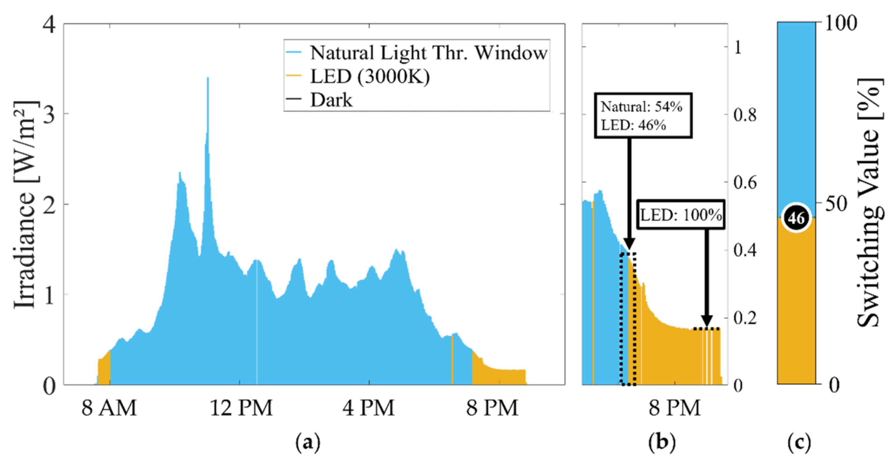
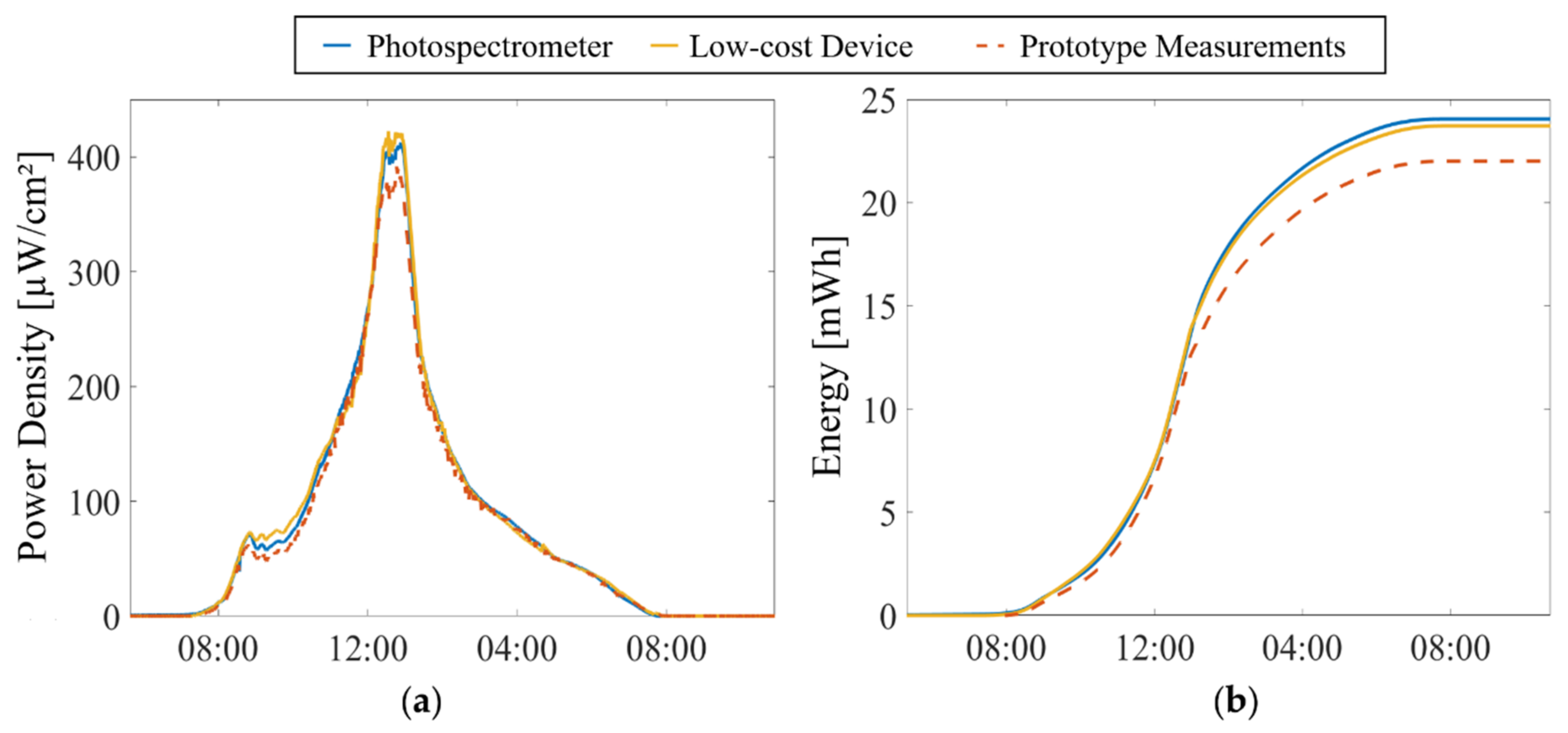
4.2. Harvestable Energy Calculation Results Using the Low-Cost Sensor

Finally, with a complete system outputting reconstructed spectra, the calculation model results may be studied. The low-cost system is tested over a period of 16 consecutive days. For comparison purposes, the compact spectrometer is installed next to the prototype. Those tests’ goal is to verify whether the classification and spectrum reconstruction processes are reliable and consistent. Figure 12a,b displays power and energy calculation results made by the model based on the compact spectrometer readings (blue line), based on the low-cost system (yellow line), and in red dashed line practical measurements made by the prototype, respectively. More results for other days are gathered in Figure S7 from the Supplementary Materials. These measurements were conducted by the energy harvesting prototype placed near the two analysis devices. The fine KNN classification method was used in association with the feature configuration R and the B normalization. For a given day presented in the figure, the error between energy harvestable calculations based on the spectrum reconstruction process and the compact spectrometer is only 1.4%. Over the sixteen-day observation samples, this mean absolute percentage error on the energy harvestable is 3.4%. This confirms that the light source classification method, combined with the spectra reconstruction, can provide model calculation results with a similar level of accuracy to results described in Politi et al. [19], which used an expensive compact spectrophotometer. This is an encouraging result and it suggests that this method could compete with a higher resolution measurement system. This level of accuracy, for a system using a relatively simple computational model and a low-cost measurement device, shows its potential as an interesting method to aid in evaluating the sizing needed for an energy recovery device to be able to make a consumer device self-sufficient.

As a proof of concept, a graphical interface, described in Figure S8, shows how these results could be exploited by a user. The main results of the calculations of the harvestable energy as well as the minimum surface area and number of solar cells (GaAs solar cells in our example) to compensate for the consumption of the electric device to supply in energy are displayed. As an example, the recommendation after 16 days of observation is to use 283 cm² of GaAs solar cells to supply energy to a wireless e-ink tablet consuming an average of about 10 mW per day.

5. Conclusions

In this work, we explored, for the first time, an ultra-low-cost light sensor device capable of estimating the harvestable energy in real indoor conditions. This device, coupled with supervised learning methods of classification, can be a powerful low-cost alternative to other more conventional methods of light characterization. This low-cost system is able to guide PV sizing with precision comparable to a system using an expensive spectrometer. The mean absolute error percentage between experimentally harvested light energy by a harvesting prototype and the model calculation based on spectrometer data or the low-cost device is lower than 6%. To go further, tests over longer periods must be realized to ensure that this system could apply its calculations throughout the year, regardless of variations in light due to seasonal changes. By implementing more precise/complex calculation models, a larger number of different PV technologies could also be added into our database to give the user their choice of solar cells. For further improvements, the development of a digital twin of the sensor could help with correction of its readings. Finally, our proof of concept works for the moment using a computer with MATLAB for pre- and post-processing. By minimizing the energy required to use a classifier, it would be feasible to operate classification processes directly on our measurement system, as demonstrated in the work of Micheals et al. [22], and even to train a classifier in an embedded way.

As said, many improvements could be done, but we believe our work opens an opportunity for engineers and researchers to deploy many autonomous devices in indoor conditions by using this method.

References

1. Carvalho, C.; Paulino, N. On the Feasibility of Indoor Light Energy Harvesting for Wireless Sensor Networks. Procedia Technol. 2014, 17, 343–350. [Google Scholar] [CrossRef] [Green Version]
2. Wang, Y.; Liu, Y.; Wang, C.; Li, Z.; Sheng, X.; Lee, H.G.; Chang, N.; Yang, H. Storage-Less and Converter-Less Photovoltaic Energy Harvesting with Maximum Power Point Tracking for Internet of Things. IEEE Trans. Comput. Des. Integr. Circuits Syst. 2015, 35, 173–186. [Google Scholar] [CrossRef]
3. Huld, T.; Müller, R.; Gambardella, A. A new solar radiation database for estimating PV performance in Europe and Africa. Sol. Energy 2012, 86, 1803–1815. [Google Scholar] [CrossRef]
4. Randall, J.F.; Jacot, J. Is AM1.5 applicable in practice? Modelling eight photovoltaic materials with respect to light intensity and two spectra. Renew. Energy 2003, 28, 1851–1864. [Google Scholar] [CrossRef] [Green Version]
5. Sarik, J.; Kim, K.; Gorlatova, M.; Kymissis, I.; Zussman, G. More than meets the eye—A portable measurement unit for characterizing light energy availability. In Proceedings of the 2013 IEEE Global Conference on Signal and Information Processing, Austin, TX, USA, 3–5 December 2013; pp. 387–390. [Google Scholar] [CrossRef]
6. Kasemann, M.; Kokert, J.; Torres, S.M.; Ruhle, K.; Reindl, L.M. Monitoring of indoor light conditions for photovoltaic energy harvesting. In Proceedings of the 2014 IEEE 11th International Multi-Conference on Systems, Signals and Devices, SSD 2014, Barcelona, Spain, 11–14 February 2014. [Google Scholar] [CrossRef]
7. Minnaert, B.; Veelaert, P. A Proposal for Typical Artificial Light Sources for the Characterization of Indoor Photovoltaic Applications. Energies 2014, 7, 1500–1516. [Google Scholar] [CrossRef] [Green Version]
8. Li, Y.; Grabham, N.J.; Beeby, S.P.; Tudor, M.J. The effect of the type of illumination on the energy harvesting performance of solar cells. Sol. Energy 2015, 111, 21–29. [Google Scholar] [CrossRef]
9. Ma, X.; Bader, S.; Oelmann, B. Characterization of Indoor Light Conditions by Light Source Classification. IEEE Sens. J. 2017, 17, 3884–3891. [Google Scholar] [CrossRef]
10. Randall, J.F. On the Use of Photovoltaic Ambient Energy Sources for Powering Indoor Electronic Devices, Ph.D. Thesis. Ecole Polytechnique de Lausanne, Lausanne, Switzerland, 2003. [CrossRef]
11. Bader, S.; Ma, X.; Oelmann, B. One-diode photovoltaic model parameters at indoor illumination levels—A comparison. Sol. Energy 2019, 180, 707–716. [Google Scholar] [CrossRef]
12. Muller, M.; Wienold, J.; Walker, W.D.; Reindl, L.M. Characterization of indoor photovoltaic devices and light. In Proceedings of the 34th IEEE Photovoltaic Specialists Conference (PVSC), Philadelphia, PA, USA, 7–12 June 2009; pp. 000738–000743. [Google Scholar] [CrossRef]
13. Hande, A.; Polk, T.; Walker, W.; Bhatia, D. Indoor solar energy harvesting for sensor network router nodes. Microprocess. Microsystems 2007, 31, 420–432. [Google Scholar] [CrossRef]
14. Afsar, Y.; Sarik, J.; Gorlatova, M.; Zussman, G.; Kymissis, I. Evaluating photovoltaic performance indoors. In Proceedings of the 38th IEEE Photovoltaic Specialists Conference (PVSC), Austin, TX, USA, 3–8 June 2012; pp. 1948–1951. [Google Scholar] [CrossRef]
15. Teran, A.S.; Wong, J.; Lim, W.; Kim, G.; Lee, Y.; Blaauw, D.; Phillips, J.D. AlGaAs Photovoltaics for Indoor Energy Harvesting in mm-Scale Wireless Sensor Nodes. IEEE Trans. Electron Devices 2015, 62, 2170–2175. [Google Scholar] [CrossRef]
16. Mathews, I.; King, P.J.; Stafford, F.; Frizzell, R. Performance of III–V Solar Cells as Indoor Light Energy Harvesters. IEEE J. Photovoltaics 2016, 6, 230–235. [Google Scholar] [CrossRef]
17. Freitag, M.; Teuscher, J.; Saygili, Y.; Zhang, X.; Giordano, F.; Liska, P.; Hua, J.; Zakeeruddin, S.M.; Moser, J.-E.; Grätzel, M.; et al. Dye-sensitized solar cells for efficient power generation under ambient lighting. Nat. Photon. 2017, 11, 372–378. [Google Scholar] [CrossRef]
18. Tinsley, N.F.; Witts, S.T.; Ansell, J.M.R.; Barnes, E.; Jenkins, S.M.; Raveendran, D.; Merrett, G.V.; Weddell, A.S. Enspect: A complete tool using modeling and real data to assist the design of energy harvesting systems. In Proceedings of the 3rd International Workshop on Energy Harvesting & Energy Neutral Sensing Systems, Seoul, South Korea, 1 November 2015; pp. 27–32. [Google Scholar] [CrossRef] [Green Version]
19. Politi, B.; Parola, S.; Gademer, A.; Pegart, D.; Piquemil, M.; Foucaran, A.; Camara, N. Practical PV energy harvesting under real indoor lighting conditions. Sol. Energy 2021, 224, 3–9. [Google Scholar] [CrossRef]
20. Ma, X.; Bader, S.; Oelmann, B. Power Estimation for Indoor Light Energy Harvesting Systems. IEEE Trans. Instrum. Meas. 2020, 69, 7513–7521. [Google Scholar] [CrossRef]
21. Beck, P.S.A.; Atzberger, C.; Høgda, K.A.; Johansen, B.; Skidmore, A.K. Improved monitoring of vegetation dynamics at very high latitudes: A new method using MODIS NDVI. Remote Sens. Environ. 2006, 100, 321–334. [Google Scholar] [CrossRef]
22. Michaels, H.; Rinderle, M.; Freitag, R.; Benesperi, I.; Edvinsson, T.; Socher, R.; Gagliardi, A.; Freitag, M. Dye-sensitized solar cells under ambient light powering machine learning: Towards autonomous smart sensors for internet of things. Chem. Sci. 2020, 11, 2895–2906. [Google Scholar] [CrossRef] [PubMed] [Green Version]
Figure 1. Descriptive diagram of the operational energy harvesting estimation method and its validation process. This method is based on multiple datasets created beforehand. The first one consists of successfully trained classifiers used to classify measurements made by the low-cost device (Classification Process) as one light class known (i.e., natural light through a window [NLTW], LED or CFL). The second one is the set of reference spectra taken while creating the training data for the classifiers. It is used to reconstruct a new spectrum from the class determined previously. The last dataset is composed of measurements made on the PV converter to be used. These data, associated with the reconstructed spectrum, can be fed to the calculation model for the final step of the method, the energy harvesting estimation.
Energies 15 01144 g001
Figure 2. (a) the compact sensor (analysis system tool) that gives light information via photodiodes dedicated to the broadband spectra, the infrared, the red, the green and the blue; (b) information collected and sent via an ESP32; (c) typical pseudospectra obtained under different light sources like CFL, LED or natural light through a window (NLTW).
Energies 15 01144 g002
Figure 3. Picture of the experimental setup: (1) two GaAs solar cells from Alta Devices Inc.; (2) Power Management Integrated Circuit (PMIC) from e-PEAS; (3) Lithium-polymer battery of 4.4 Wh; (4) energy-consuming devices; (5) INA219 power measurement integrated circuits from Texas Instruments; (6) ESP32 microcontrollers, in charge of gathering and storing data, integrated on HUZZAH Feather boards made by Adafruit; (7) OLED display to show system operating state.
Energies 15 01144 g003
Figure 4. Results of training classifiers on the raw data set. The classification success varies drastically depending on the classification method used. The best results are achieved with Cubic SVM, Fine KNN and Weighted KNN. The choice of the data features configuration has a less significant impact on the training results.
Energies 15 01144 g004
Figure 5. Representation of the 126 observations in the raw dataset. (a) Each observation is positioned according to the R and IR values. Decision surface of (b) the Cubic SVM classification method and (c) the Fine KNN classification method, both using I data configuration. Decision surfaces of the four best classifiers are shown in the Supplementary Figure S1.
Energies 15 01144 g005
Figure 6. Results of the classifiers training using difference normalization. (a) Representation of the 126 observations using normalization to B value. Light source observations are very distinctly separated. (b) Applying the Fine KNN method, its decision surface exhibits a significant improvement with very clear zones for each light source class.
Energies 15 01144 g006
Figure 7. Performance of different classifiers trained through a 5-fold cross validation process with the B normalization.
Energies 15 01144 g007
Figure 8. Summary of classifiers and configurations reaching 100% correct classification, all normalizations combined.
Energies 15 01144 g008
Figure 9. (a) Controlled light environment used to create generalization test data for classifiers that passed the training test. (b) Classification results using normalization by B value (B normalization) in a controlled light environment.
Energies 15 01144 g009
Figure 10. (a) Classes recognized for a day with mixed light sources using Fine KNN method, associated with the R data configuration; (b) Switching moment between natural light and LED light classes; (c) Switching ratio value between those two classes.
Energies 15 01144 g010
Figure 11. (a) Light intensity values given by the TSL2561 sensor in lux; values normalized to the lux value given by the spectrometer. Values from the sensor depend on the type of light source and its intensity and can induce errors. (b) Evolution of the low-cost system’s light intensity measurement error as a function of the spectrometer’s reference light intensity. Measurements made during a whole day in an environment mainly lit by natural light passing through a window. Selection of different natural light sources to add to the classification system for greater accuracy.
Energies 15 01144 g011
Figure 12. Result of the reconstruction method, after implementing a more accurate correction of the measured values by the low-cost light intensity system (a) Power density and (b) Energy harvested according to model calculations (solid lines) or prototype measurements (dashed line).
Energies 15 01144 g012