Article

Optimal Tradeoff between MPP and Stability of a PV-Based Pumping System

1
Laboratory of Automation, Electrical System and Environment (LAESE), National Engineering School of Monastir, Monastir 5019, Tunisia
2
Department of Computer Engineering, College of Computers and Information Technology, Taif University, P.O. Box 11099, Taif 21944, Saudi Arabia
3
Department of Electrical Engineering, Higher Colleges of Technology, Ruwais Campus, Abu Dhabi 12389, United Arab Emirates
*
Author to whom correspondence should be addressed.
Energies 2022, 15(3), 1106; https://doi.org/10.3390/en15031106
Submission received: 23 December 2021 / Revised: 28 January 2022 / Accepted: 28 January 2022 / Published: 2 February 2022
(This article belongs to the Special Issue Grid and Photovoltaic Powered Pumping Systems)

Abstract

:
This paper presents a novel algorithm to pick PV-based pumping system operating points that simultaneously achieve maximum delivered power and optimized stability. We present an in-depth analysis of operating point dynamics and shape the PV output current and voltage parameter plans. Accordingly, we draw the power bifurcation diagram with all possible operating points. Our proposed algorithm picks the power operating point midway between two consecutive stable points and far enough from the stability boundary to assure system safety. We validated our methodology successfully by numerical simulation based on speculative evidence using MATCON/MATLAB/SimPowerSystems blocks. In addition, we compared the proposed algorithm with P&O MPPT algorithm, and the results verified the reliability of our proposed algorithm to deliver maximum stable power.

1. Introduction

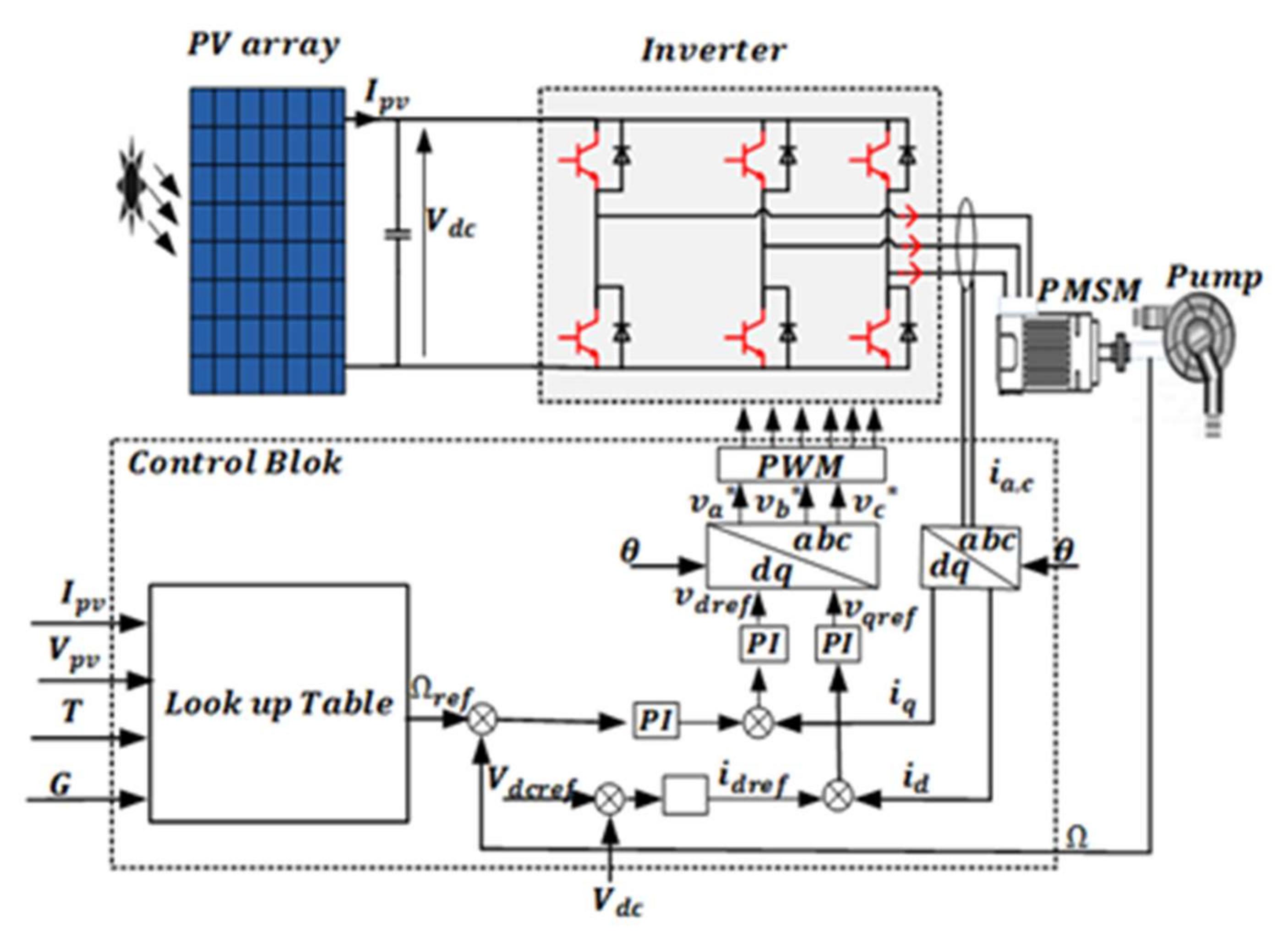
Photovoltaic (PV) power systems are one of the most economical sources for water pumping in rural areas. The importance of PV power systems is due to their affordability, reliability, and maintenance. However, photovoltaic systems’ complexity comes from photovoltaic modules and switching-mode converters possess nonlinearity and time-variant characteristics. Generally, a PV generation system consists of a photovoltaic array, maximum power point tracking (MPPT) controller, DC/AC converter, and the associated controllers. Hence, the entire model is a nonlinear multivariate system, and its performance depends on weather conditions.
PV generators could be coupled directly to the pumping systems, standalone, or connected to the battery. The latter is an optimal choice from the stability point of view as it provides a fixed amount of power. Meanwhile, the stored energy would be available at nighttime. However, although researchers have been working to tackle such a problem, energy storage is an expensive option. In contrast, a direct connection to the pumping system is preferable since it saves some money. However, delivered power is subject to fluctuation and loss due to the susceptibility of PV energy.
MPPT is a common problem in PV energy systems to increase power extraction efficiency. It is crucial for any PV generator system, such as a PV pumping system, to minimize losses and to improve the entire system performance [1,2,3,4]. Even though MPPT is an efficient technique to harvest energy, the stability of the electromechanical part of the pumping system will be affected by power operating points. The electromechanical part is composed of an electric motor and pump. For each of them, the meaning of stability must be well defined. For the latter, usually, water pressure and flow rate should be within a certain limit. In contrast, the stability of the former is based on current, voltage, and motor angular speed. Consequently, the stability of the coupled system, motor and pump, should be consistent with PV operating points. For instance, the paper [5] developed a PV drip irrigation system that has many orifices fed by a pump controlled by a motor to keep pressure and flow at some values. Therefore, motor angular speed should be governed by choosing desired voltage operating point. On the other hand, the optimal voltage that runs the system at MPP might affect pump stability in terms of pressure and flow. Thus, possible improvement of system performance could be achieved if the system is studied from a wide-angle and considers the said points. To understand all components’ effects on the system stability, the authors calibrated the motor voltage and the pump pressure in a standalone PV drip irrigation system. They analyzed the system performance under different environmental conditions. The results showed that the stability of the hydraulic system is affected by fluctuation of PV generator environmental parameters, irradiance and temperature. Many studies have been performed in the literature based on tracking MPP through power electronics converters, DC/DC or DC/AC, such that the global system is stable at some operating points [6,7,8]. However, the tradeoff between MPP and stability should be optimized.
The relationship between MPP and stability under the effect of different parameters should be well understood. Analytically, it is not simple to find such a relationship, as there is no easy analytical solution for such a complicated system. Therefore, studying system behavior under varying parameters, bifurcation, is of interest for many researchers as different system characteristics can be presented. For instance, the papers [9,10,11] investigated how parameter variation can affect stability, and they design controllers accordingly. Moreover, in complicated power conversion systems, they are usually connected to multi-input energy sources, and they can work in a different mode with different structures. Consequently, the dynamics of the overall system are complicated, and the effect of changing parameters might be investigated to determine stable operating points for each structure and operation mode [12,13,14].
In pumping systems, we need to evaluate the behavior of the overall system under varying parameters, temperature and irradiance, to find optimal operating points that jointly achieve MPP and optimized stability. Therefore, we proposed a new control strategy based on stability-constraint power maximization problem. The proposed optimization problem is formulated as a minimization cost function of photocurrent. Precisely, the cost function is the product of output power, between critical points, by the real part of dominant eigen values of the entire system at each instant of photocurrent. This cost function must be continuous in photocurrent to ensure the existence of local minima. The photocurrent that achieves local minima of such a function is the optimal operating point that ensures MPP and reasonable stability simultaneously. Our contribution can be summarized in the following steps:
  • We investigate the parameter dynamics of the global system.
  • We introduced a power bifurcation diagram based on the PV output current and voltage plane analysis.
  • By a novel proposed algorithm, we determine the system optimal operating points that jointly achieve MPP and stability.
This paper starts with the subsystem models to formulate the global system model with the problem formulation in Section 1. We identify and discuss parametric singularities in parameter planes of the PV output current and voltage in Section 2. In Section 3 we present the set of operating points on power bifurcation diagrams. Section 4 proposes an algorithm to search for operating points that achieve optimal tradeoff between MPP and stability. Finally, we conclude this paper by comparing our proposed method and P&O algorithm results in Section 5.

2. System Modeling

2.1. Mathematical Formulation

Typically, the integrated PV pumping system consists of photovoltaic modules, a boost converter, inverter, PMSM, and centrifugal pump, as shown in Figure 1.
Physically, a simple PV generator can be modeled with a diode, two resistors, and a current generator, as shown in Figure 2. Mathematically, Equations (1)–(3) represent the generated current by a single PV cell [15,16].
I p v = I L I 0 e x p V d c + R s p v I p v A 1
I p v is the solar-generated current, which can be solved implicitly with a numerical iterative method, Newton–Raphson, for example, knowing that:
I L = G G r e f I L , r e f + μ I s c T c T r e f
I 0 = I 0 , r e f T T r e f 3 e x p n s E q A 1 T c , r e f T c
Indeed, PV-generated current is affected by irradiance variability. Consequently, DC voltage might be subject to fluctuations, required to be regulated at a certain level. Therefore, a simple proportional controller can be used for reference current tracking as in Equation (4), resulting in controlled DC voltage:
i d r e f = k p d c v d c r e f v d c
where i d r e f is the d-axis reference current of the inverter, k p d c is the proportional control gain, and Vdc is DC-link capacitor voltage which is, according to the power balance principle, equivalent to the generated voltage, Vdc = Vpv, and expressed as follows:
C d v d c d t = i p v 3 2 v d v d c i d
where v d and i d are the d-axis PMSM voltage and current, respectively. PMSM is modeled with a smooth air gap so that d-q winding inductances are equal. The following mathematical model describes the dynamics of PMSM itself:
d i d d t = R s L d i d + p L q L d i q Ω + 1 L d v d d i q d t = R s L q i q p L d L q i d Ω p ϕ f L q Ω + 1 L q v q d Ω d t = f J Ω + p . m L d L q 2 J i d i q + p . m ϕ f 2 J i q T r J
If PMSM is designed at a low-rated voltage level, the PV array can be directly connected to the DC/AC inverter, and the MPPT is achieved by adjusting motor speed and current. The adjustment of motor velocity and its current can be made by the PWM switching technique that drives the DC-AC inverter with modulation index M [16]. Thus, the fundamental motor voltage, Vm, is given as:
V m = M V 2
The modulated waveform results from subtracting control signal from constant number, usually one, that eventually compared with the carrier wave and triangle wave, to generate pulses as drivers of DC/AC inverter gates. On the other hand, the control signal is the signal that is sent by the controller to correct the difference between actual and reference values. The PI controller is a popular controller that can be used for this purpose, which is defined as follows:
C P I t = k p ε t + k i 0 t ε t d t
where ε t = x r e f x (t), is the control error, x r e f is the reference value, and x (t) is the vector of machine state variables. In the light of this equation, d-q reference voltages, V = ( v d r e f ,   v q r e f ) , are generated by three PI regulators as follows:
v d r e f = k p i d r e f i d + k i I i d
v q r e f = k p i q r e f i q + k i I i q
With:
I i d = 0 t i d r e f i d d t
I i q = 0 t i q r e f i q d t
where Iid and Iiq are the current regulators, and the PI regulator of angular speed can obtain the reference current as in Equation (13):
i q r e f = k p w Ω r e f Ω + k i w 0 t Ω r e f Ω d t
Now, let’s define the integral speed regulator of the system as follows:
I w = 0 t Ω r e f Ω d t
Then substitute Equations (5), (11), (12) and (14) into Equations (9), (10) and (13), yields:
v d r e f = k p k p d c v d c r e f v d c i d + k i I i d
v q r e f = k p k p w Ω r e f Ω + k i w I w i q + k i I i q
i q r e f = k p w Ω r e f Ω + k i w I w
Differentiating Equations (11), (12) and (14) to t, results in the following differential system:
d I i d d t = k p d c v d c r e f v d c i d
d I i q d t = k p w Ω r e f Ω + k i w I w i q
d I w d t = Ω r e f Ω
Eventually, the output d,q motor voltages V m = v d ,   v q become:
v d = M 2 v d r e f
v q = M 2 v q r e f
The last part of our integrated system is the centrifugal pump, which is characterized by its load torque Tr. The load torque is proportional to the square of motor rotor speed:
T r = A p ω r 2
where ( A p = P n ω n 3 ) is the torque constant, P n is the nominal power of the PMSM, and ω n is the rotor nominal speed. Putting everything together results in the global mathematical model, which is described by seven differential equations and one algebraic equation as follows:
{ d i d d t = R s L i d + p i q Ω + M 2 L k p k p d c v d c r e f v d c i d + k i I i d d i q d t = R s L i q p i d Ω p ϕ f L Ω + M 2 L k p k p w Ω r e f Ω + k i w I w i q + k i I i q d Ω d t = f J Ω + K T i q A p Ω 2 J d I i d d t = k p d c v d c r e f v d c i d d I i q d t = i q k p w Ω + k i w I w + k p w Ω r e f d I w d t = Ω r e f Ω C d v d c d t = I p v 3 M 2 2 k p k p d c v d c r e f V d c i d + k i I i d v d c g I L , I 0 , V d c , R s p v , A = I p v = I L I 0 e x p V d c + R s p v I p v A 1
The entire system in Equation (24) is highly nonlinear; to study its behavior under parameters variation, we first find the equilibrium points by equating the right-hand sides of Equations (24) to zero, resulting in Equation (25):
{ I i d e = 2 L M k i p A p Ω r e f 2 + f Ω r e f J K T Ω r e f I i q e = 2 L M k i p ϕ f L Ω r e f + R s L A p Ω r e f 2 + f Ω r e f J K T i q e = A p Ω r e f 2 + f Ω r e f J K T i d e = 0 I w e = A p Ω r e f 2 + f Ω r e f k i w J K T Ω =   Ω r e f   I p v e = 3 M 2 2 k i v d c r e f 2 L M k i p A p Ω r e f 2 + f Ω r e f J K T Ω r e f   I L e = I p v e + I 0 e x p v d c r e f + R s p v I p v e A 1 v d c = v d c r e f
The next step is to investigate the parameters such as index modulation, current, voltage, temperature, and rotor speed on system stability. The following section provides a comprehensive analysis of parametric singularities and bifurcation sets.

2.2. System Analysis

In nonlinear dynamical systems, sometimes, it is not easy to find an explicit solution. Instead, we study the equilibrium point’s stability, periodicity, and topological structure in the parameter plane. For instance, the complete system in Equation (25) might be subject to irradiance and temperature fluctuations leading to a readjustment of the controller signal to get the suitable driving pulses that ensure reference tracking. However, good tracking depends on controller design and operating points. If the former is perfect, then the chosen operating points should be stable and far enough from critical points to assure system stability with smooth tracking. Therefore, we represent the effect of modulation index variation on motor angular velocity in Figure 3. The setpoint of angular speed must be between two stable boundary points with enough distance to maintain system safety. From the figure, bifurcation occurs at points LP1 and LP2 with corresponding modulation indices M1 = 1.11 and M2 = 0.13, respectively, to create the boundaries for stability.
In a PV solar system, ambient temperature plays an essential role in the amount of output power and its stability. Output current is a function of photovoltaic current, voltage, and other variables. Unfortunately, not all operating points under different temperatures are stable, resulting in unstable current, voltage, and power. Therefore, to determine hazardous regions of photovoltaic current and DC voltage to temperature variation, we varied the ambient temperature and drew the corresponding current and voltage in the plan, as shown in Figure 4. From the figure, stability regions were separated by one saddle-node, LP, at T = 2.32 °C with eigenvalues λ 1 , 2 = 4260.96 ± j 615.99 ,   λ 3 = 331.15 ,   λ 4 = 0 .
To set the voltage at desired nominal value, it should be in the stable region, which decays exponentially with increased temperature, as shown in Figure 4a. On the other hand, the stable photovoltaic current must be increased proportionally with higher temperature to preserve system stability, as shown in Figure 4b.
The maximum power point tracking was done by adjustment of PV parameters, current or voltage control. Therefore, proportional control gain varied to define stability boundaries, as shown in Figure 5 The control gain profile splits DC voltage curve into stable and unstable segments within small intervals. The saddle-node LP was obtained at k p d c = 0.971 with associated eigenvalues λ 1 , 2 = 4170.14 ± j 615.42 ,   λ 3 = 131.19 ,   and   λ 4 = 0 . Hopf bifurcation point, H , occurred at k p d c = 1.1 with associated eigenvalues λ 1 , 2 = 4497.46 ± j 620.73 , and one conjugate pair of purely complex roots at λ 3 , 4 = ± j 130.9 .
Moreover, Figure 6 shows that Hopf bifurcation occurred under varying temperatures from low to high with a slight change of proportional controller gain.
Bifurcation diagrams of Figure 5 and Figure 6 confirm that the proportional controller kept voltage stable everywhere except at two boundary points. On the other hand, lower proportional gain resulted in higher output voltage and vice versa. Therefore, these observations should be considered when designing the controller.

3. The Proposed Algorithm

The main goal is to select operating points that achieve an optimal tradeoff between delivering the maximum power and stability. If the objective controller is only extracting maximum power, then operating points that achieve this goal might be on the boundary of system stability, leading to impaired reliability. In contrast, strong stable points may compromise the amount of delivered power. Therefore, we propose a new methodology to select operating points midway between the points that maximize output power and achieve strong stability. Let’s define three types of operating points:
  • The maximum power operating point (MPP) at which the maximum power is delivered by the PV system, regardless of stability.
  • The operating point (OP) is placed equidistant from the closest critical points, regardless of the power level.
  • The optimal operating point (MPOP) is placed midway between the MPP and OP points to ensure both stability and delivering sufficient power.
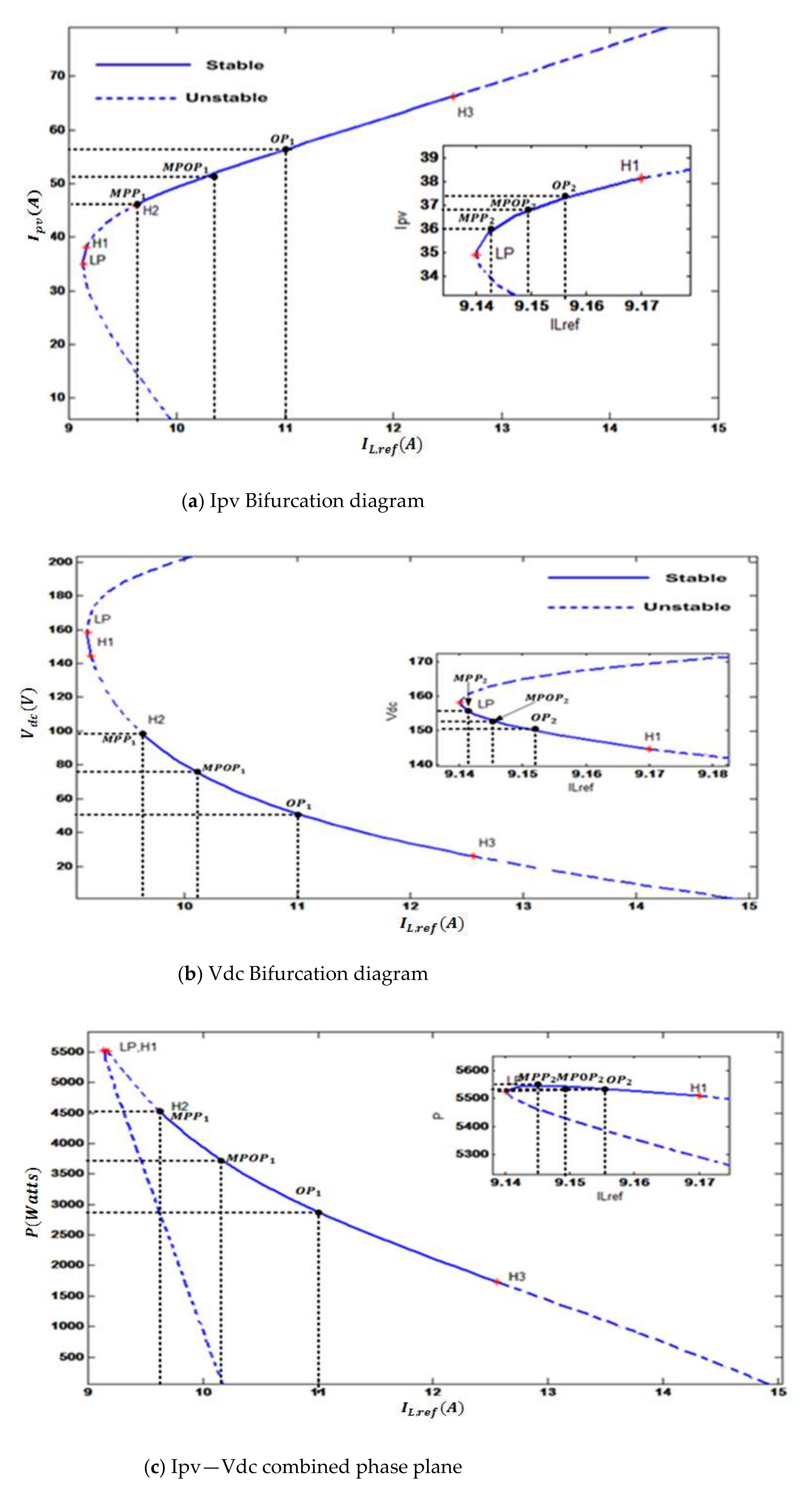
A stability assessment of the entire system needs eigenvalues estimation, which is often computationally expensive for multiple parameters. Therefore, few effective parameters are selected to investigate the parametric singularities and to inspect the anomalous behaviors. We mainly studied the photocurrent on stability and produced power as it is the control parameter that was considered in this work. In other words, we varied output current and observed the change in the output voltage, as shown in Figure 7 To elaborate, assume Figure 7b, at temperature T = 25° and irradiance G = 200 watt/m2, we have one saddle-node, LP, and three critical Hopf points, H1, H2 and H3, with an associated dominant pair of complex conjugate eigenvalues. To find the optimal operating point, MPOP, we must find OP and MPP first, then MPOP will be placed midway between them to ensure that the system works far enough from critical points and outputs a fair amount of power. The figure shows two stable regions bounded by pairs of critical points (LP, H1) and (H2, H3). Possibly, MPOP could be in either region. Therefore, two points of OP (OP1, OP2) and two MPP (MPP1,MPP2) points should be determined for region1 and region2, respectively. OP points in both regions are placed far enough from critical points, namely, midway of each pair of critical points, so that the system won’t be subject to a harmful response. Consequently, MPOP in each region (MPOP1, MPOP2) were chosen to be midway between the pairs of (OP1, MPP1) and (OP2, MPP2), respectively, as shown in Figure 7b.
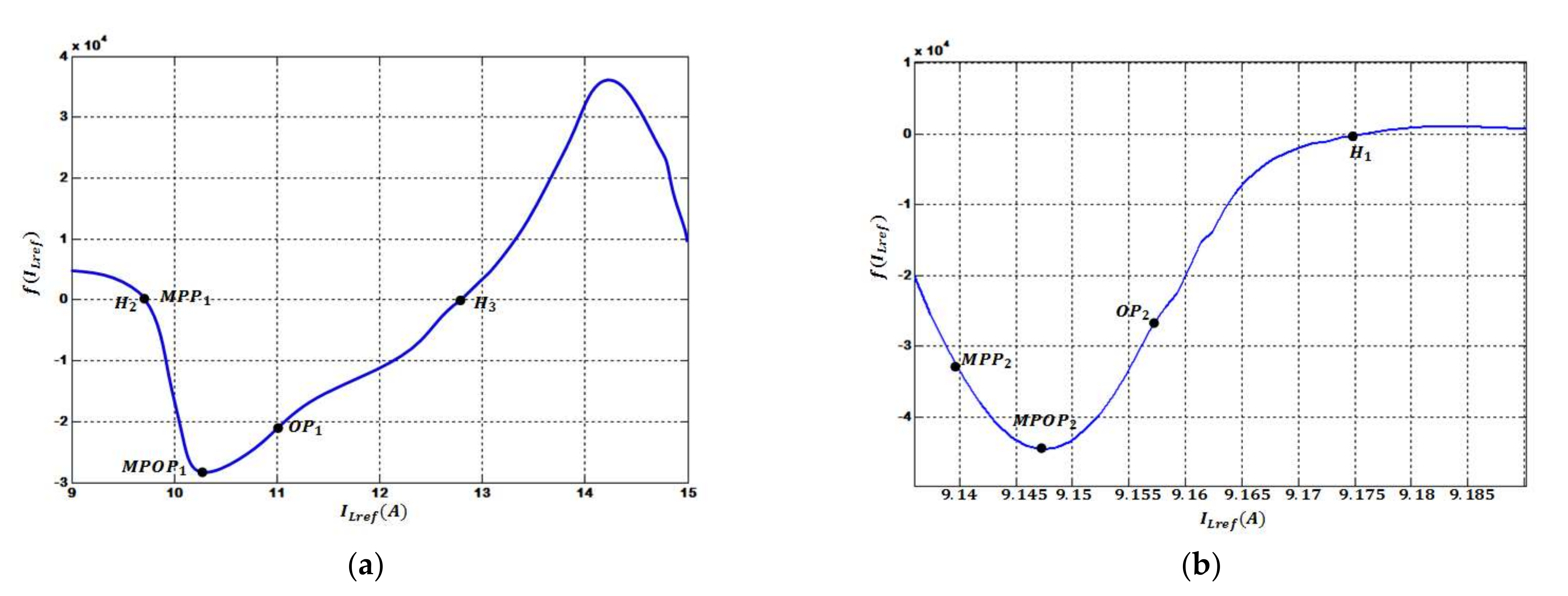
We claim that this methodology of selecting MPOP results in optimal trade-off between stability and maximum power delivery. To validate our claim, MPOP can be estimated speculatively as local minima of the cost function. Such a function is the product of all instant amount of power between critical points by the real part of the dominant eigenvalue of states 2 and 4, iq and id, respectively, in Equation (24), which are denoted as λ 2 , 4 . In other words, the cost function for each stable region is computed by varying photocurrent. At each instant photocurrent, we found corresponding power, the dominant eigenvalues λ 2 , 4 , and the product of power by the real part of dominant eigenvalues λ 2 , 4 . This cost function must be continuous in photocurrent to ensure the existence of local minima. In our system, cost function in the first region, J1, was computed by taking the instant output power between critical points H2 and H3 and multiplying it by the corresponding real part of λ 2 , 4 . Samwise, in the second region, instant output power between critical points H1 and LP were multiplied by the real part of dominant eigenvalue λ 2 , 4 to form cost function, J2. The general form of this minimization cost function is as follows:
J i = f   I L k = min k = n m P ( I L k )   .   r e a l   λ 2 , 4   k   i = 1 , 2
Such that
I L c 1     I L k     I L c 2
where I L k is the photocurrent at time k, P ( I L k ) is the corresponding output power at a given photocurrent, I L c 1 and I L c 2 are lower and upper bounds, respectively, of photocurrent at both critical points. Figure 8 represents both cost functions (f(IL1), f(IL2)) for region1 and region2, respectively. MPOP1 and MPOP2 label local minima for both functions at IL1 = 10:4 A and IL2 = 9:15 A, respectively, which can be easily verified from Figure 9c.
The result that we concluded is based on a specific amount of temperature and irradiance, T = 25° and G 200 watt/m
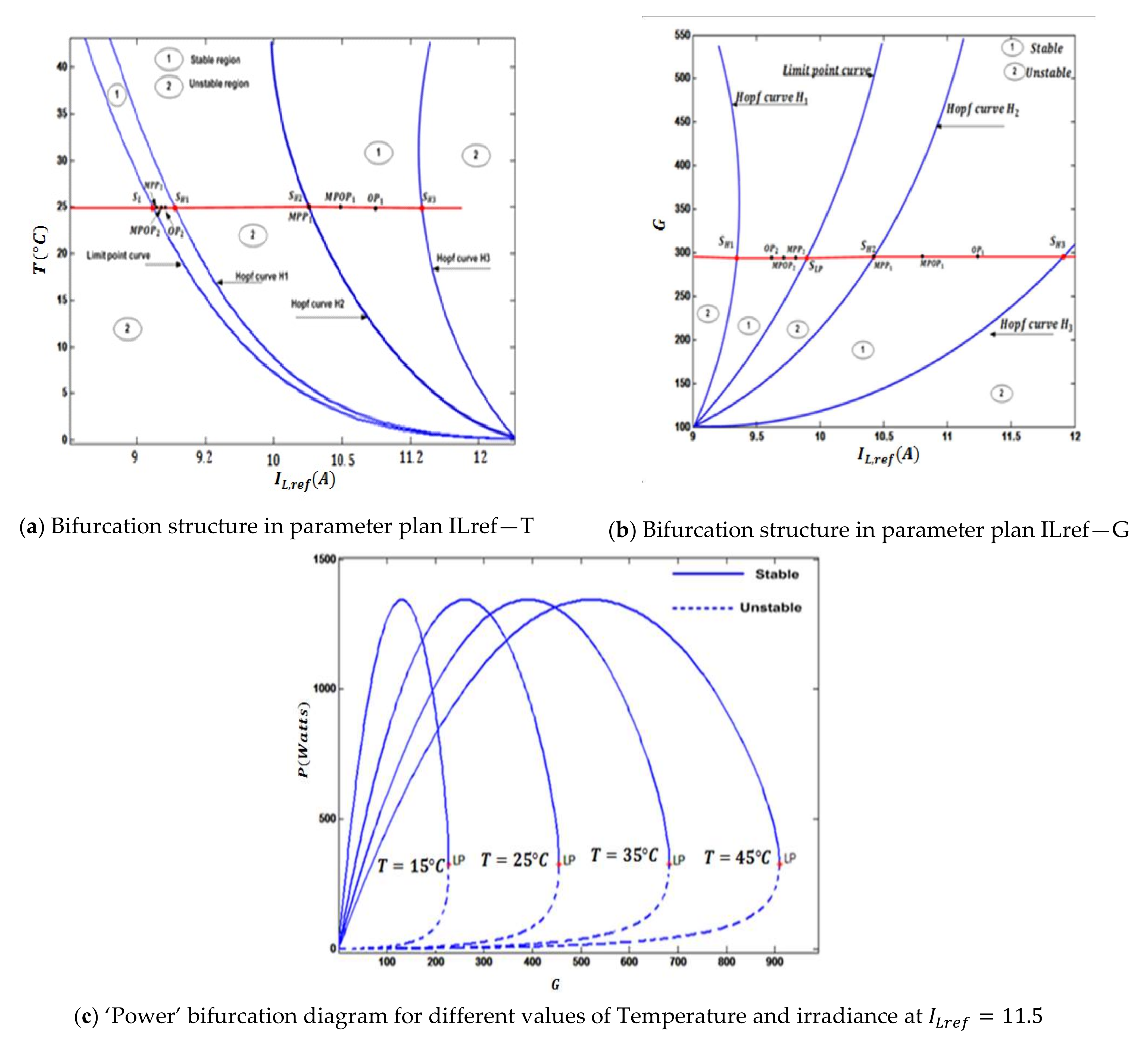
2. However, those parameters are varying over time, and they could be any different combination. Consequently, stable regions and corresponding cost functions were subject to change, resulting in varying local minima and, hence, different MPOP placement. Therefore, we repeated the procedure of selecting MPOP under temperature and irradiance variations, and the results are shown in Figure 9. Figure 9a, and Figure 9b show curves split regions into stable, labeled with the number 1, and unstable, labeled with the number 2. Finding MPOP was achieved using the same explained technique at each instant amount of temperature and irradiance in stable regions. For example, to help find MPOP at T = 25° and G = 300 watt/m2, red lines were drawn horizontally. Their intersections with curves determine corresponding critical points and associated eigenvalues that contribute to cost function implementation. Temperature degrees and the strength of irradiance directly affected operation regions. Increasing those parameters results in critical points spacing and distinguishable regions that help to decide MPOP positioning. For instance, at each instant of temperature and irradiance, the system displayed more than one stable region, resulting in multiple MPOP placements in each region. Only one of them should be nominated to be the optimal operating point. In our proposed method, the one associated with a widen stable region, with enough distance between two critical points, was selected for safety assurance.
At a specific photocurrent, the right combination of temperature and irradiance led to analogous output power. In Figure 9c, photocurrent was fixed at 11.5 amperes, and the output power was a function of temperatures and irradiance. At low degrees of temperature, maximum power could be reached with a minimal amount of irradiance. On the other hand, with increased temperature, a higher amount of irradiance was required to achieve the same amount of output power, which is reasonable by the principle of PV power generation. Unfortunately, such parameters are uncontrollable, and the right choice of MPOP requires knowing the effect of parameters variation on the complete range of photocurrent. In other words, Figure 9c should be recreated for each instance of current and ILref; MPOP was determined based on the actual reading of irradiance, temperature, and the optimal current that balanced between MPP and reliable stability. In real-time, MPOP should be determined at any combination of PV parameters. Therefore, a dataset might be collected experimentally, and then an online solution can be found using machine learning tools.
To recap, our proposed methodology of finding MPOP passes through the following steps:
  • Step 1: Define the basic design parameters, I L r e f ,   I o r e f ,   T r e f ,   T c ,   T c , r e f ,   I m p , r e f ,   V m p , r e f ,   V o c , r e f ,   T ,   G r e f ,   and   G , see Table 1.
  • Step 2: Using the PV pumping system model (24), compute the equilibrium points and their eigenvalues.
  • Step 3: based on step 2, find phase planes, and identify stable regions for IPV and Vdc according to ILref variation.
  • Step 4: from IPV and Vdc phase planes, draw the output power phase plane.
  • Step 5: Define the MPP and the OP points on the power bifurcation diagram and derive the MPOP. The corresponding DC voltage value is chosen from ILrefVdc Phase plane as in Figure 8.
  • Step 6: For DC voltage regulation, the corresponding proportional gain can be defined from the k p d c v d c phase plane as in Figure 5.

4. Validation and Results

To validate our proposed algorithm, we compare our proposed algorithm against Perturb and Observe algorithm, P&O, in terms of stability and extracted power. Use of this algorithm is a common technique to track maximum power point in the PV system. P&O only extracts MPP by adjusting the output voltage at the DC/DC converter regardless of the other system components. Although P&O is an efficient algorithm for power extraction, it does not consider system stability. The simulation results show that our proposed algorithm offers a good alternative that balances power extraction and system stability.
We set up MATLAB/Simulink with shown parameters in Table 1 [17]. We assumed a fixed amount of temperature, T = 25°, as the change in temperature was slow compared to the change in the light intensity, which might fluctuate rapidly. Therefore, simulation started with initial illumination, G = 30 watt/m2, and changed to 500, 100, and 800 watt/m2 at the 1st, 3rd and 6th second, respectively. According to these values, motor velocity should be set at 150, 50 and 180 rad/s to track maximum power point. Performance of tracking control was evaluated under three different operating points, OP, MPP, and MPOP, in each stable region. With the current considered scenario, we found two stable regions, see Figure 7c, where we needed to evaluate our system performance with proposed operating points in both regions.

4.1. Evaluation of Operating Points in Stable Region #1

This region was sandwiched between two critical points. The operating points could be controlled with an IL current in the range of 9.6 and 12.7 A. Particularly, the maximum change of IL current in this region was 3.1 A, which is a fair amount that ensures optimal operating point placement based on the cost function explained earlier. Starting from 
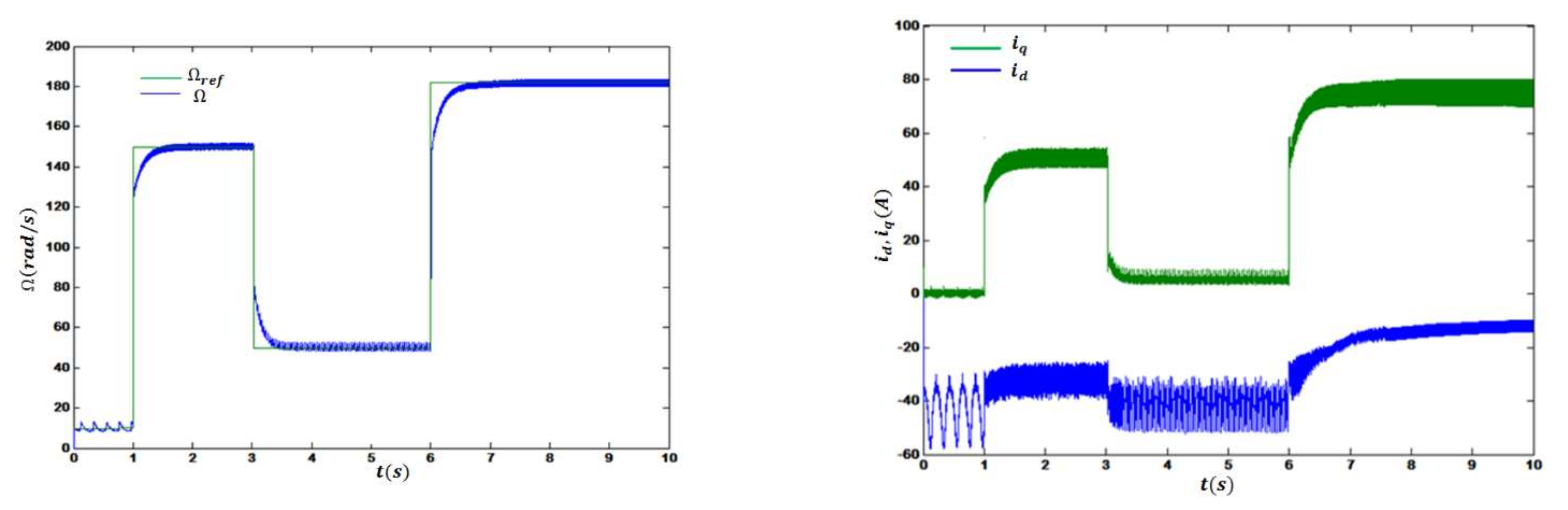
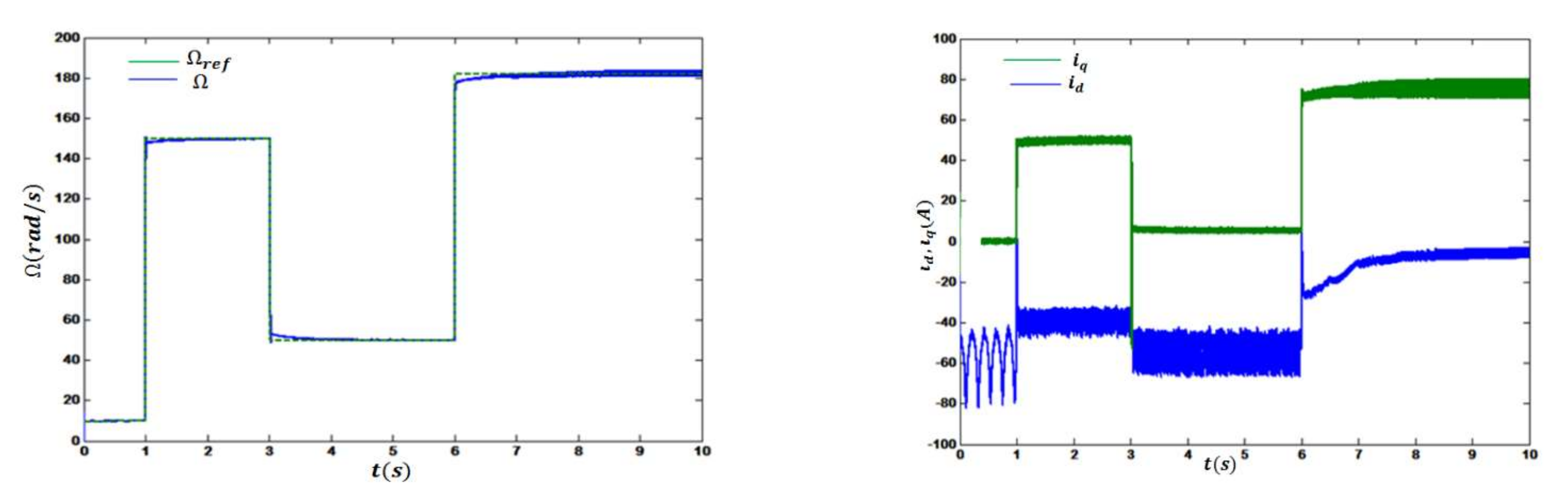
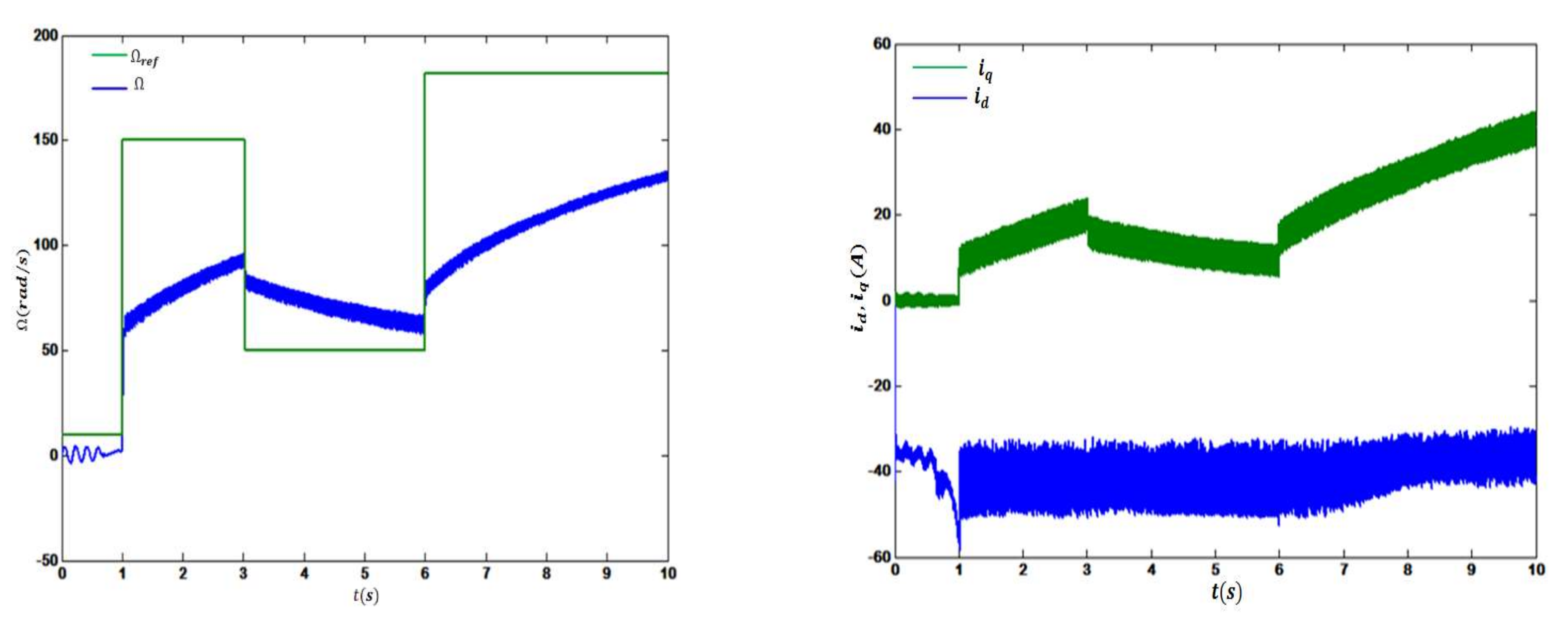
Figure 10 the PV PMSM system operates at the point OP1. The transitions of the motor speed and stator currents are shown in this figure. At the third second, the iq current of the PMSM was negative when the speed changed from 150–50 rad/s because PMSM operates in generator mode. Moreover, the stator currents were reduced because of vector control with the q-axis reference current, Iq. The figure shows that dynamics with OP1 were acceptable in terms of oscillation because of its distance from critical points. However, results showed a loss of some amount of delivered power.
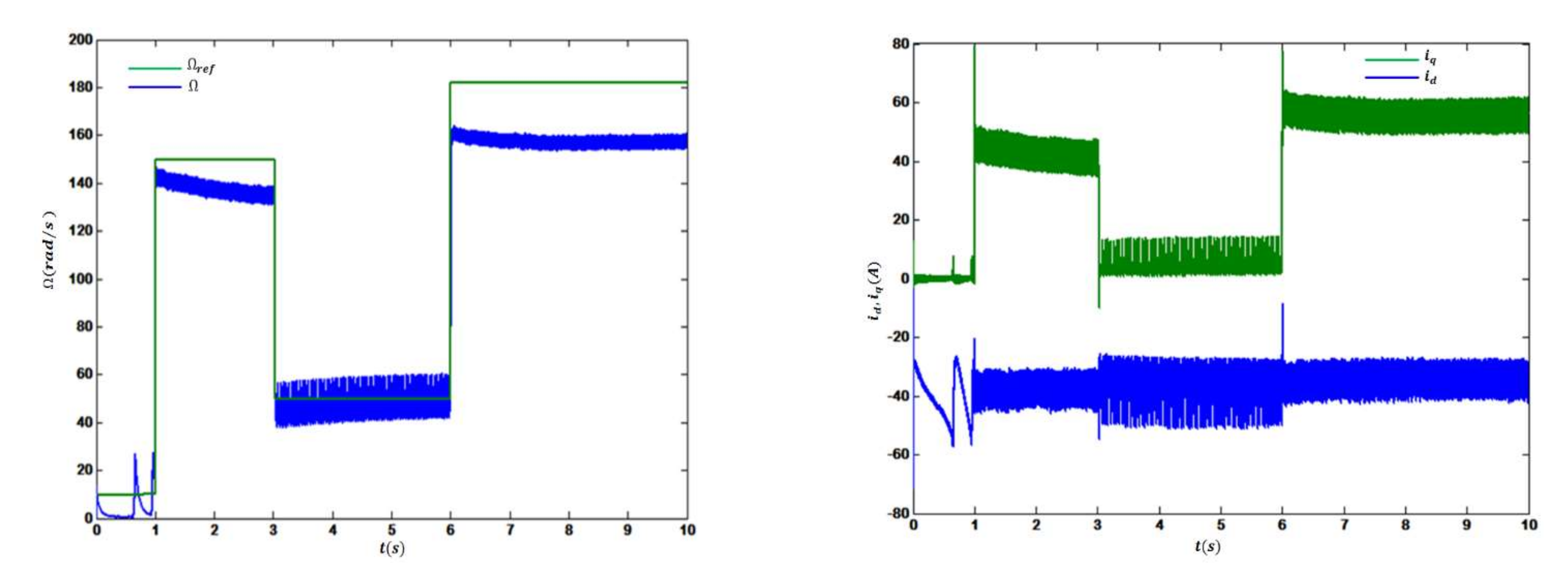
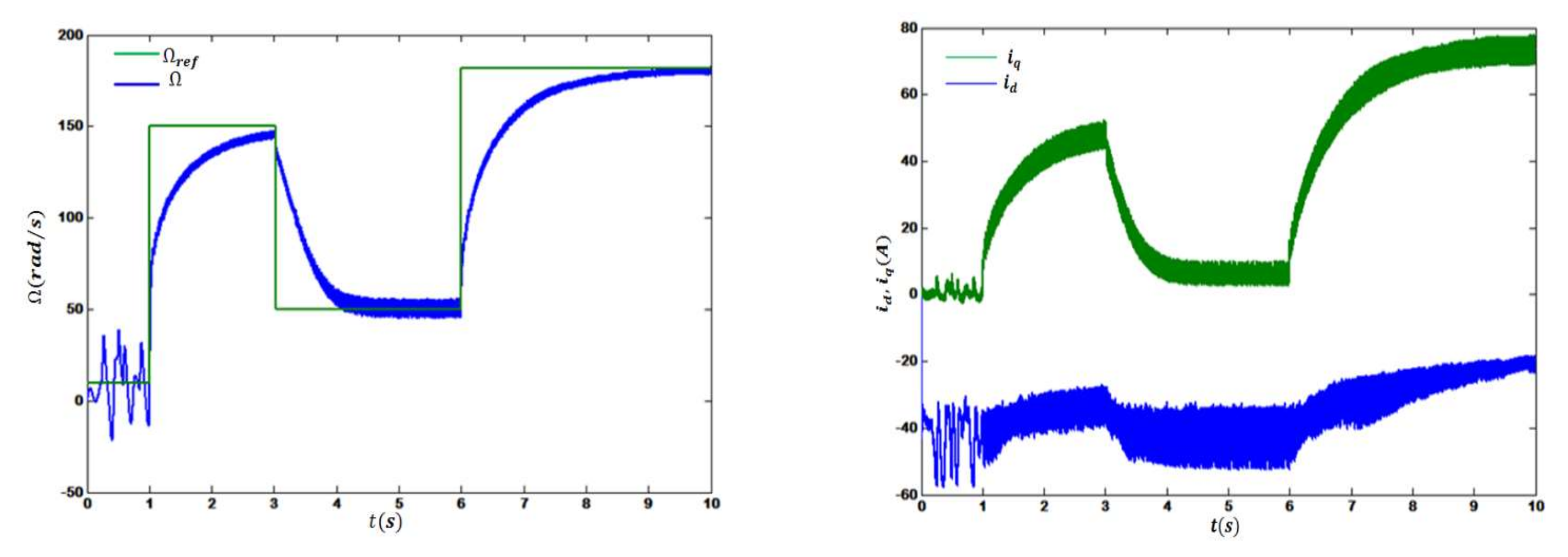
Figure 11 explains that, by changing the operation point to MPOP1, the system’s performance could be ameliorated. System dynamics associated with the operating point MPOP1 were optimal in terms of stability and maximum delivered power, reducing oscillation, and better reference tracking. The effect of the operating point location was obvious on the stator current, where little variation in rotor speed showed a significant impact on it. In contrast, dynamics with MPP1 resulted in a tolerant amount of delivered power, although oscillation increased due to the location of the point MPP1, see Figure 12. Comparing part b of Figure 10, Figure 11 and Figure 12 tells us that closeness of operating point from critical points resulted in distortional current.

4.2. Evaluation of Operating Points in Stable Region #2

In this narrow region, the transient system from stable to unstable state was susceptible to change in IL current. In other words, little change in IL, at a scale of milliampere, or even slight perturbation in initial conditions, might lead to destabilized system dynamics. Therefore, work in this region is risky and may result in unpleasant performance. As shown in
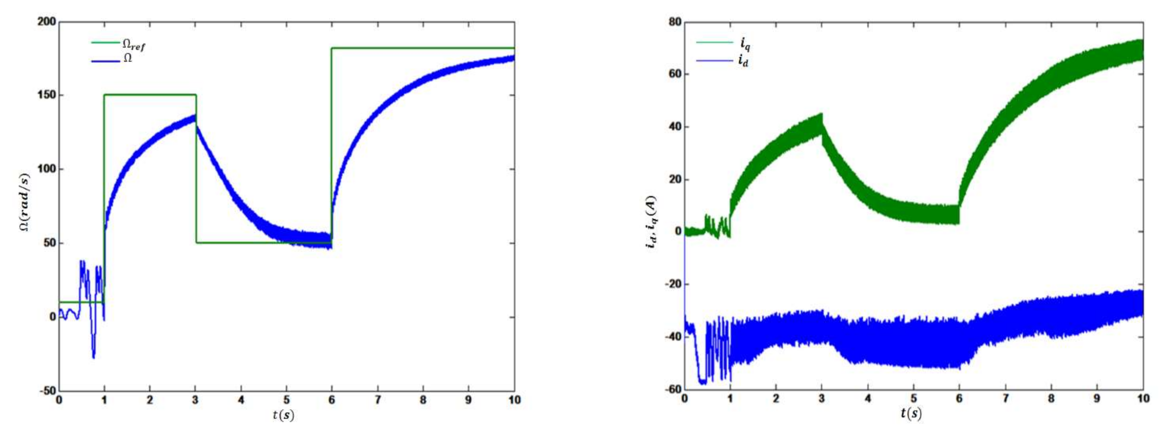
 Figure 13 and Figure 14, both operating points, OP2 and MPOP2, showed a similar effect on reference tracking control and the consequent stator current. However, due to its location midway between two critical points, OP2 was located at the furthest possible distance from those points. Consequently, running the system at this operating point improved tracking control slightly, although general performance was imperfect compared to running the system at OP1 in region1. In contrast, MPOP2 was placed midway between MPP2, which is close to the critical point, and OP2, causing MPOP2 to be pushed up toward the stability boundary. Therefore, it is not surprising to have found a worse control performance than when the system runs at OP2. The worst-case scenario is when MPP2 is chosen to be operating point wherein the quality of reference tracking is inferior, resulting in wasting delivered power and undesirable system vibration, as shown in Figure 15. In all cases, the points OP2, MPOP2, and MPP2 were located in distances of milliampere from each other. Such an arrangement causes the validation of our proposed algorithm to be difficult in this region. Hence, no optimal tradeoff solution could be found.
In conclusion, if we possess a system with multiple stable regions, and to get the best of our proposed algorithm, the region that guarantees placement of MPOP at enough distance from critical points is selected where the sensitivity of stability to the current variation in this region is minimal.

4.3. Comparison between Conventional MPPT and Proposed Algorithm

In this subsection, we need to study the system behavior when tracking maximum power with two different approaches, 1—using conventional P&O algorithm to track MPPT regardless of stability, 2—using our proposed algorithm that balances stability and maximization of delivered power. Initially, simulation starts with assumed light intensity G = 530 watt/m2 and changes to G = 550 watt/m2 and G = 510 watt/m2 at the third and 6th second with corresponding generator speeds that achieve maximum power extraction, 100, 110, and 90 rad/s, respectively. 
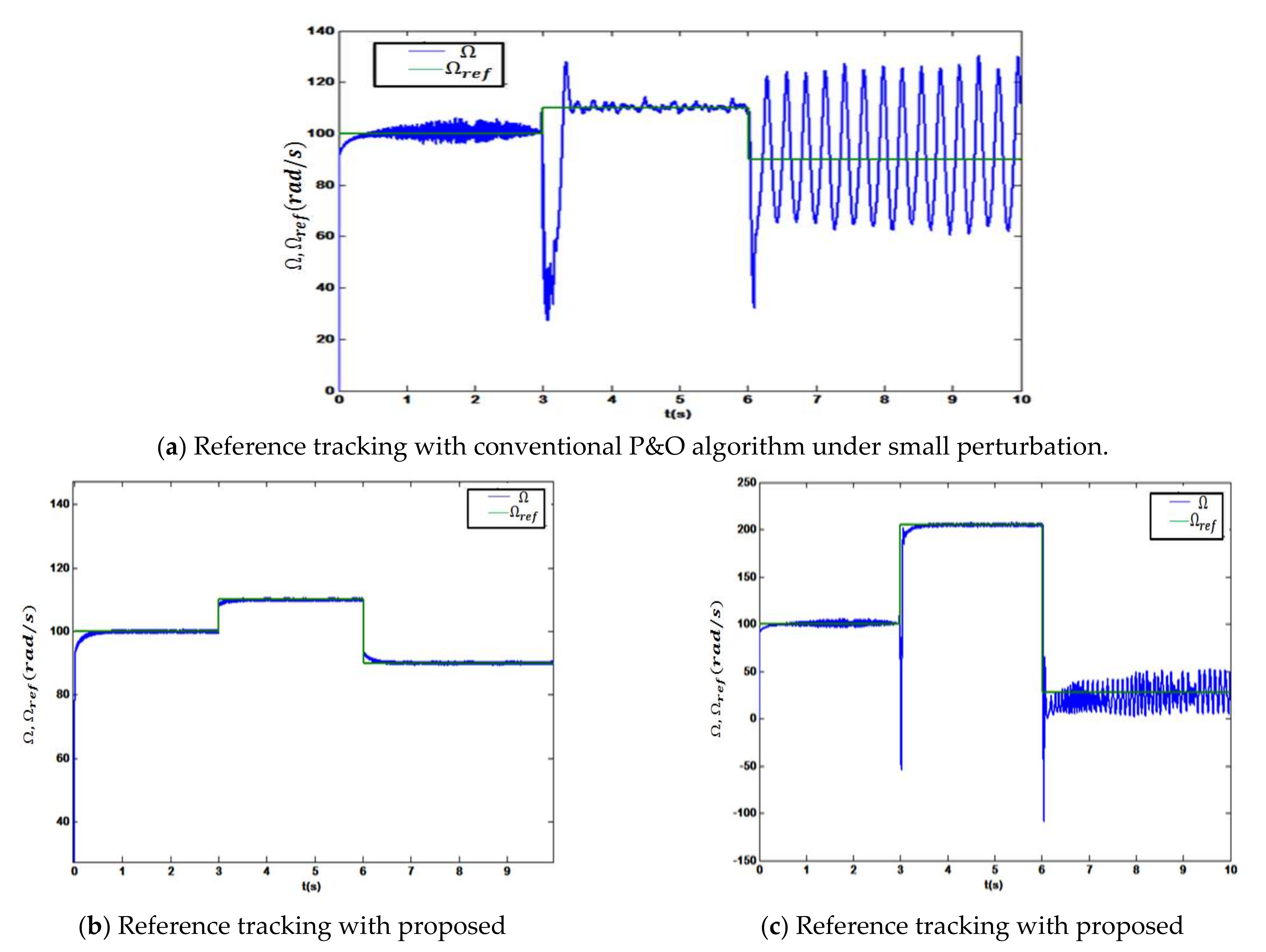
Figure 16a shows generator velocity tracking with the conventional MPPT algorithm, wherein the operating point chosen by this algorithm, MPP1, is close to the critical point. Therefore, the system starts tracking velocity at 100 rad/s, initially, with rapid swinging around the reference signal. The first perturbation occurred at the 3rd s when the reference speed changed from 100 up to 110 rad/s. Even though the change in generator speed was slight, 10 rad/s, it caused a big undershoot, and the system took about 0.5 s to catch up with the reference speed. Tracking became worse when the second perturbation occurs at the 6th second. Reference speed changed from 110 down to 90 rad/s, which was a bigger change than the first perturbation. In this case, the system become closer to the critical point associated with pure complex conjugate eigenvalues. Therefore, the system started oscillating between those values; any further change in the same direction might have led to unstable operation.
In contrast, with our proposed algorithm, the operating point, MPOP1, was far enough from the critical point. When a minor disturbance occurred, it was rejected faster with desirable transience, as shown in Figure 16b. To investigate the impact of significant disturbance on the system behavior, we repeated simulation with G = 530, 830, and watt/m2 with the corresponding generator speeds 100, 200, and 25 rad/s, respectively, as shown in Figure 16c. The first change occurred at the 3rd second with the difference of 100 rad/s about the initial speed. In this case, the control system can still mitigate the effect of this big jump. The figure showed perfect tracking of the generator speed, which means that the system was delivering maximum power steadily. Generator speed fell from 200 down to 25 rad/s at the 6th second, with 175 rad/s about the previous speed. Indeed, this was a huge difference, and may have drug operating points away from equilibrium points and, hence, avoided linear control functionality. However, the proposed algorithm ensures that the huge perturbation effect will be mitigated due to a good selection of operating points, as shown in the same figure.

5. Conclusions

We introduced a novel approach for delivering maximum power within optimal operating points. We started with global system modeling and studying its dynamics around equilibrium points. We were able to construct a power phase plane based on current and voltage bifurcation diagrams. We determined stable regions. We took the real parts of dominant eigenvalues between critical points in the power phase plane and multiplied them by the output power to construct a cost function that needed to be minimized. We showed that the minimum value of cost function was the optimal operating point that achieved a tradeoff between maximization of delivered power and stability. The proposed algorithm was validated in different operating regions, and a comparative study was conducted between conventional MPPT and our proposed algorithm. The results showed that our algorithm provided a better solution for power extraction and system stability simultaneously.

Author Contributions

Conceptualization, W.S. and S.A.; methodology, W.S. and H.K.; software, W.S.; validation, S.A., W.S. and H.K.; formal analysis, S.A.; investigation, S.A. and H.K.; resources, W.S. and I.A.; data curation, I.A.; writing—original draft preparation, S.A., W.S. and H.K.; writing—review and editing, I.A.; visualization, W.S.; supervision, H.K. and I.A.; project administration, S.A. and H.K.; funding acquisition, S.A. All authors have read and agreed to the published version of the manuscript.

Funding

This work was supported by Taif University Researchers Supporting Project number (TURSP-2020/348), Taif University, Taif, Saudi Arabia.

Institutional Review Board Statement

Not applicable.

Informed Consent Statement

Not applicable.

Data Availability Statement

Not applicable.

Acknowledgments

The author would like to thank Taif University for supporting this research.

Conflicts of Interest

The authors declare no conflict of interest.

Nomenclature

I p v PV generatorcurrent (A)
I L Photocurrent (A)
I L , r e f photocurrent at standard rating conditions (A)
I 0 reverse saturation current (A)
I 0 , r e f reverse saturation current at standard rating conditions (A)
V d c Output generator dc voltage (V)
v d c r e f Dc voltage reference (V)
R s p v Cells resistances of PV (Ω)
L d d -axis self-inductance of the stator (H)
L q q -axis self-inductance of the stator (H)
R s Stator resistance per phase (Ω)
M Modulation index
ω = p Ω Motor angular speed (rad/s)
Ω r e f Angular reference speed(rad/s)
T temperature of the PV cell (K)
T r e f temperature of the panel at standard rating conditions (25 °C–298.15 K)
T c temperature of the photovoltaic device (K)
T c , r e f photovoltaic device temperature at reference condition
G Solar irradiance (W/m2)
G r e f solar irradiance at standard rating conditions (1000 W/m2)
A the diode quality factor
n s Number of cells in series
E q the band gap energy of the semi-conductor (eV)
I m p , r e f current at the maximum power point at standard rating conditions (A)
V m p , r e f voltage at the maximum power point at standard rating conditions (V)
V o c , r e f open circuit voltage of the panel at standard rating conditions (V)
μ V o c thermal coefficient of the open circuit voltage (V/°C)
μ I s c thermal coefficient of the shortcircuitcurrent (A/°C)
k p Proportional regulator of PMSM current
k p w Proportional regulator of PMSM speed
k p d c Proportional regulator of PV dc voltage
k i Integral regulator of PMSM current
k i w Integral regulator of PMSM speed

References

  1. Talbi, B.; Krim, F.; Rekioua, T.; Mekhilef, S.; Laib, A.; Belaout, A. A high-performance control scheme for photovoltaic pumping system undersudden irradiance and load changes. Sol. Energy 2018, 159, 788–795. [Google Scholar] [CrossRef]
  2. Al-Hindawi, M.; Abusorrah, A.; Al-Turki, Y.; Giaouris, D.; Mandal, K.; Banerjee, S. Nonlinear Dynamics and Bifurcation Analysis of a Boost Converter for Battery Charging in Photovoltaic Applications. Int. J. Bifurc. Chaos 2014, 24, 1450142. [Google Scholar] [CrossRef]
  3. Khaehintung, N.; Kunakorn, A.; Sirisuk, P. A Novel Fuzzy Logic Control Technique tuned by Particle Swarm Optimization for Maximum Power Point Tracking for a Photovoltaic System using a Current-mode Boost Converter with Bifurcation Control. Int. J. Control. Autom. Syst. 2010, 8, 289–300. [Google Scholar] [CrossRef]
  4. Xiong, X.; Tse, C.; Ruan, X. Smooth and Non-smooth Bifurcations in Multi-structure Multi-operating mode Systems: Case Study of a Power Conversion System with Two Energy Sources. Fifth Int. Workshop Chaos-Fractals Theor. Appl. 2012, 23, 1350094. [Google Scholar]
  5. El Khazane, J.; El Houssaine, T. Achievement of MPPT by finite time convergence sliding mode control for photovoltaic pumping system. Sol. Energy 2018, 166, 13–20. [Google Scholar] [CrossRef]
  6. Caracas, J.; Farias, G.; Teixeira, L.; Ribeiro, L. Implementation of a High Efficiency, High-Lifetime, and Low-Cost Converter for an Autonomous Photovoltaic Water Pumping System. IEEE Trans. Ind. Appl. 2014, 50, 631–641. [Google Scholar] [CrossRef]
  7. Feraga, C.; Bouldjedri, A. Performance of a Photovoltaic Pumping System Driven by a Single Phase Induction Motor Connected to a Photovoltaic Generator. Automatika 2016, 57, 163–172. [Google Scholar] [CrossRef] [Green Version]
  8. Haroun, R.; El Aroudi, A.; Cid-Pastor, A.; Garıca, G.; Olalla, C.; Martınez-Salamero, L. Impedance Matching in Photovoltaic Systems Using Cascaded Boost Converters and Sliding-Mode Control. IEEE Trans. Power Electron. 2015, 30, 3185–3199. [Google Scholar] [CrossRef]
  9. Deivasundari, P.; Uma, G.; Poovizhi, R. Analysis and experimental verification of Hopf bifurcation in a solar photovoltaic powered hysteresis current-controlled cascaded-boost converter. IET Power Electron. 2013, 6, 763–773. [Google Scholar] [CrossRef]
  10. Dubey, M.; Sharma, S.; Saxena, R. Single stage PV system based Direct Torque Controlled PMSM drive for pump load application. In Proceedings of the 2016 IEEE International Conference on Power Electronics, Drives and Energy Systems (PEDES), Kerala, India, 14–17 December 2016. [Google Scholar]
  11. Wen, X.; Ajjarapu, V. Critical Eigenvalue Trajectory Tracing for Power System Oscillatory Stability Assessment. IEEE Power Eng. Soc. Gen. Meet. 2004, 2, 1883–1889. [Google Scholar]
  12. El Aroudi, A. Out of Maximum Power Point of a PV system Because of Subharmonic Oscillations. In Proceedings of the 2017 International Symposium on Nonlinear Theory and Its Applications. NOLTA 2017, Cancun, Mexico, 4–7 December 2017. [Google Scholar]
  13. Xiong, X.; Tse, C.; Ruan, X. Bifurcation Analysis of Standalone Photovoltaic- Battery Hybrid Power System. IEEE Trans. Circuits Syst. 2013, 60, 1354–1365. [Google Scholar] [CrossRef]
  14. Betka, A.; Moussi, A. Performance optimization of a photovoltaic induction motor pumping system. Renew. Energy 2004, 29, 2167–2181. [Google Scholar] [CrossRef]
  15. Erkan Deniz, E. ANN-based MPPT algorithm for solar PMSM drive system fed by direct-connected PV array. Neural Comput. Applic 2016, 10, 3061–3072. [Google Scholar]
  16. Nabipour, M.; Razaz, M.; Seifossadat, S.; Mortazavi, S. A new MPPT scheme based on a novel fuzzy approach. Renew. Sustain. Energy Rev. 2017, 74, 1147–1169. [Google Scholar] [CrossRef]
  17. Aissa, B.; Borni, A. Improvement of synchronous and asynchronous motor drive systems supplied by photovoltaic arrays with frequency control. J. Electr. Eng. 2008, 59, 169–177. [Google Scholar]
Figure 1. PV motor pumping system.
Energies 15 01106 g001
Figure 2. Solar cell equivalent circuit.
Energies 15 01106 g002
Figure 3. Modulation index bifurcation diagram.
Energies 15 01106 g003
Figure 4. Saddle-Node bifurcation due to temperature changes. L P : x = 99.4 , 0.23 , 204.9 , 120.6 ,   T = 2.32 , λ 1 , 2 = 4260.96 ± j 615.99 ,   λ 3 = 331.15 ,   λ 4 = 0 .
Energies 15 01106 g004
Figure 5. Bifurcation diagram in the plane ( k p d c , v d c ).
Energies 15 01106 g005
Figure 6. Hopf bifurcation curve in the parameter plane T k p d c .
Energies 15 01106 g006
Figure 7. Bifurcation diagrams at G = 200 , T = 25   ° C .
Energies 15 01106 g007
Figure 8. Evolution of function f(ILref) and stability analysis of operating points. (a) cost function for region 1; (b) cost function for region 2.
Energies 15 01106 g008
Figure 9. Bifurcation structure in varying parameter plan.
Energies 15 01106 g009
Figure 10. PMSM performance for different reference speed ω r e f = 10 ,   150 and 180 r a d / s for the operating point O P 1 , and for T = 25   ° C .
Energies 15 01106 g010
Figure 11. PMSM performance for low, middle and high reference speed for the maximum power operating point M P O P 1 , and for T = 25   ° C .
Energies 15 01106 g011
Figure 12. PMSM responses for the maximum power point M P P 1 , and for T = 25   ° C .
Energies 15 01106 g012
Figure 13. PMSM performance for different reference speed ω r e f = 10 ,   150 and 180 rad / s , for the operating point O P 2 , and for T = 25   ° C .
Energies 15 01106 g013
Figure 14. PMSM performance for low, middle and high reference speed for the maximum power operating point M P O P 2 , T = 25   ° C .
Energies 15 01106 g014
Figure 15. PMSM responses for the maximum power point M P P 2 , and for T = 25   ° C .
Energies 15 01106 g015
Figure 16. Comparison of Performances of PV system between MPPT with P&O and the proposed algorithms (algorithm under tolerable perturbation. algorithm under higher perturbation).
Energies 15 01106 g016
Table 1. System parameter values.
R s p v Ω I L r e f A I 0 , r e f A v d c r e f V J L (H) R s Ω Ω r e f ( rad / s ) T r e f ( ° C ) T c ( ° C )
41510104000.0060.0111.22003050
T c , r e f ° C ) G r e f W / m 2 n s E q e V I m p , r e f V m p , r e f V o c , r e f V μ V o c V / ° C μ I s c V / ° C k p
45500111.24.2516.9 V21.5 82.10 3 3.10 3 1.1
k p w k p d c k i k i w
0.71.3210
Publisher’s Note: MDPI stays neutral with regard to jurisdictional claims in published maps and institutional affiliations.

