1. Introduction
One hundred and eighty countries of the Paris Agreement set the goal to reduce CO
2 emissions and achieve near climate neutrality [
1]. The countries aim to reach a balance between greenhouse gas emissions and their removal by sinks (greenhouse gas neutrality) in the second half of the century.
In Germany, approximately 72% of the primary energy consumption of commercial buildings and 80% of residential buildings is used for heating or cooling [
2], while globally, residential and commercial buildings including the building construction sectors “are responsible for over one-third of the global end energy consumption” [
3]. Therefore, these types of buildings are of special interest in the context of sustainability [
4], and in order to achieve the previously mentioned goals, new approaches are needed. The European Energy Performance of Building Directive (EPBD) supports, for example, buildings that will be equipped with new control devices to monitor and control the indoor air quality (IAQ) [
5].
Thermal comfort and the behavior of building occupants play a crucial role in the energy balance of buildings. Buildings are often maintained with a tight “deadband” in a narrow range, in order to sustain a thermally comfortable state. However, in reality, the building occupants are often unsatisfied with these predefined conditions, and a tight deadband does not really improve comfort compared to a “wide” deadband [
6]. Furthermore, maintaining a narrow deadband frequently leads to higher energy consumption [
7], and too-cold or too-hot conditions at the workplace could lead to building-related illnesses such as sick building syndrome [
8,
9]. Besides that, the indoor environmental quality influences the productivity of employees to a large extent [
10]. It is difficult to define a perfect temperature befitting all occupants as human perception varies greatly between individuals [
11].
Thermal comfort is driven by different factors such as the personal factor of activity level (metabolic rate); the clothing insulation (winter/summer clothing); and environmental conditions such as air temperature, radiant temperature, air velocity, relative humidity, and direct solar influence. Besides clothing and activity level, the cultural and climatic backgrounds also influence thermal perception [
4]. The “Adaptive Comfort Model” [
12], which is the global standard for designing and operating naturally ventilated buildings and which is included in the ASHRAE Standard 55 [
13], considers the thermal history and climatic background of building occupants.
For the design and operation of energy-efficient buildings the occupant behavior in terms of the opening and closing of windows and behavior relating to heating and cooling (operating with heating and cooling setpoints, duration of heating/cooling phase, etc.) have a great impact on the building energy use and the indoor environment. These circumstances were studied within the Annex 66 [
14] of the International Energy Agency (IEA) and the follow-up Annex 79 [
15] for “Occupant-centric Building Design and Operation”.
To take the energy demand of buildings into account, environmental influences need to be considered in the planning process of the building and the plant systems. Often, building simulation software is used for the planning process. Some standards such as ISO 17772-1 [
16] and DIN EN 16798 [
17] specify input parameters for the design of the building envelope, heating/cooling, ventilation, and lighting calculations.
For a simplified consideration of thermal comfort aspects, thermal comfort is usually defined by the operative temperature or with Fanger’s PMV model [
18] as defined within different standards [
19,
20]. Although these are the most widely used parameters to predict comfort conditions, they do not allow detailed consideration of asymmetric conditions (e.g., solar influence via large reflective surfaces) or local (dis)comfort of humans, which affect the overall comfort [
21].
From both the thermal comfort aspect and the energy efficiency aspect, more consideration should be taken for individual body parts as the discomfort of individual body parts can determine the overall discomfort [
22,
23]. In this context, the application of decentralized heating and cooling systems in offices is interesting, as they act on the people’s immediate environment and take individual body parts into consideration. Furthermore, these systems react very fast, which solves another typical user complaint [
8,
24].
The study from Liu et al. showed that building occupants shape their working environment as a response to discomfort [
8,
25], and user satisfaction can be increased with the ability to control the direct environmental conditions around a person [
26]. The EVA project from Sommer et al. studied the “Evaluation of visionary architectural concepts—state of the art” and came to the conclusion that for 66% of the considered projects, comfort was achieved because the occupants had control over the temperature [
27].
The energy-saving effects of decentralized systems have been demonstrated in various studies [
28]. Decentralized systems are, for example, office chairs [
29,
30,
31,
32,
33,
34], fans [
35], or a thermoelectric cooling wall [
36,
37,
38]. Other systems are foot warmers [
39], heated and cooled wristpads [
40], localized floor heating [
41], desktop task conditioning systems (DTC) [
42], personalized ceiling ventilation [
43,
44,
45], and task-ambient conditioning systems consisting of palm warmers and heated keyboards [
46]. Another approach presented by Carlos Rotti [
47] includes local infrared heating elements at the ceiling combined with human presence control via motion tracking. By this, a thermal heating “cloud” could follow the human “through the space” with the aim of saving energy.
These systems are receiving more and more interest in the market, but there is a lack of planning tools. This article presents an approach using a virtual adaptive building controller, which considers detailed transient thermal comfort values of a manikin while controlling decentralized heating and cooling systems as well as the central heating and cooling system. The objectives of this development are twofold: (1) To provide a numerical tool to investigate the potential of decentralized systems to improve thermal comfort and reduce energy consumption, and (2) to encourage the use of these systems and their integration in new and innovative control strategies in buildings.
2. Decentralized Heating and Cooling Systems
ASHRAE Standard 55 defined a target of 80% occupant satisfaction. However, in practice, this is often missed because the sole use of central heating and cooling systems is not sufficient to offer all building occupants thermally comfortable conditions. Furthermore, controlling the temperature of an entire room volume to, e.g., 24 °C is highly energy-consuming.
In summary, a central heating and cooling system cannot address the following factors:
An approach that incorporates the above factors is the use of decentralized heating and cooling systems, or “Personal Comfort Systems” (PCS) [
31] or “Personal Environmental Comfort Systems” (PECS), to provide direct and personalized temperature control for occupants.
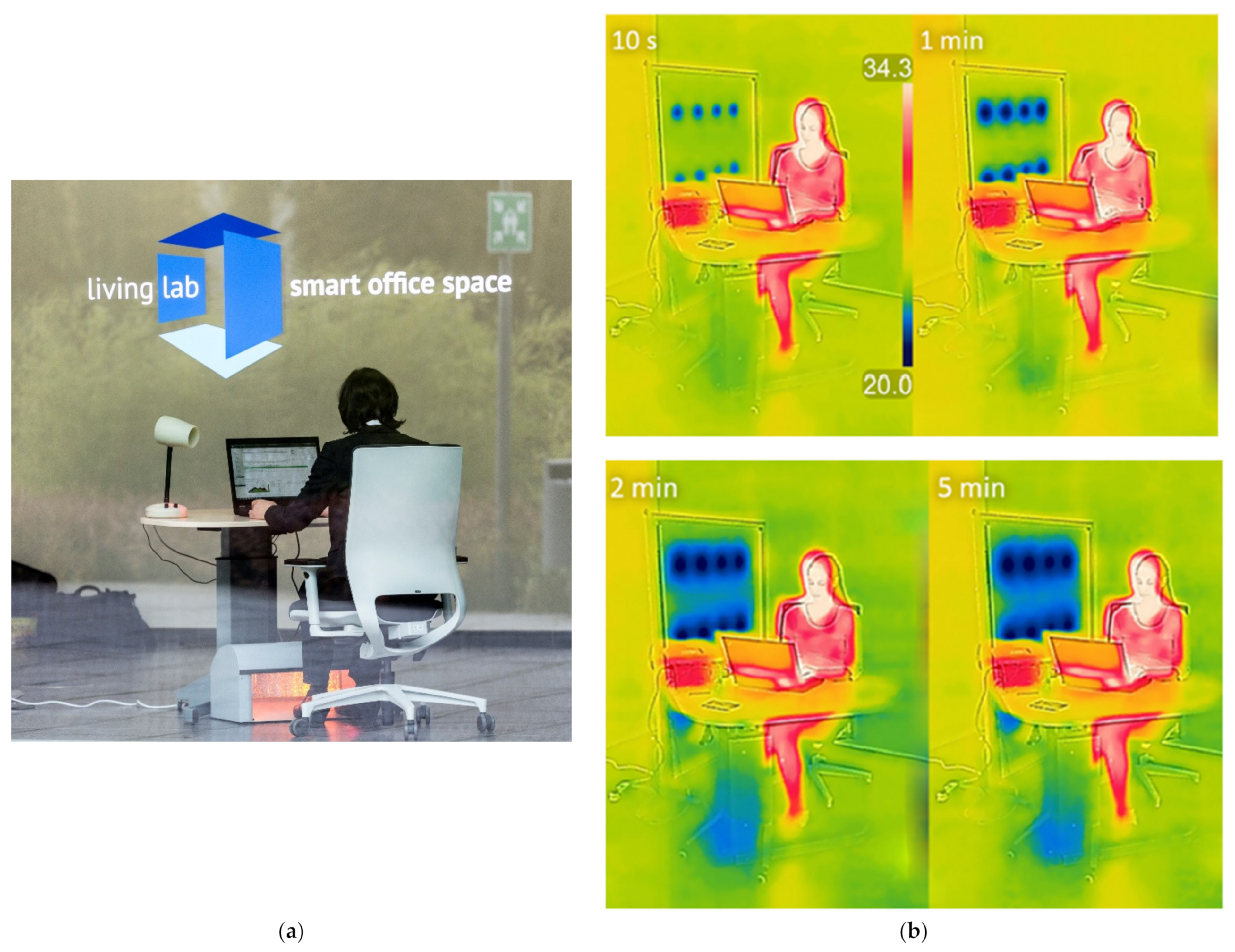
Figure 1 demonstrates a few of the previous mentioned decentralized systems that are used in the Living Lab smart office space in Kaiserslautern. The left image shows a footwarmer, a desk fan, and an office chair with a heating and cooling function, whereas the right image displays the function of the thermoelectric cooling partition directly after switching it on and after a few minutes of using the cooling function.
Advantages of Decentralized Heating and Cooling Systems
Decentralized heating and cooling systems usually have a low energy demand and address specific body parts [
33,
34,
50]. In this way, they can additionally increase the comfort of individual users and allow the range of comfortable room temperatures to be increased, which in turn helps to save energy for the central heating and cooling system [
28,
29].
The effect of “self-influence” or personalized control on the direct thermal environment also has a great psychological significance [
31]. When people have the possibility to influence the control process [
41], they experience greater comfort, by the ability to change something on their own.
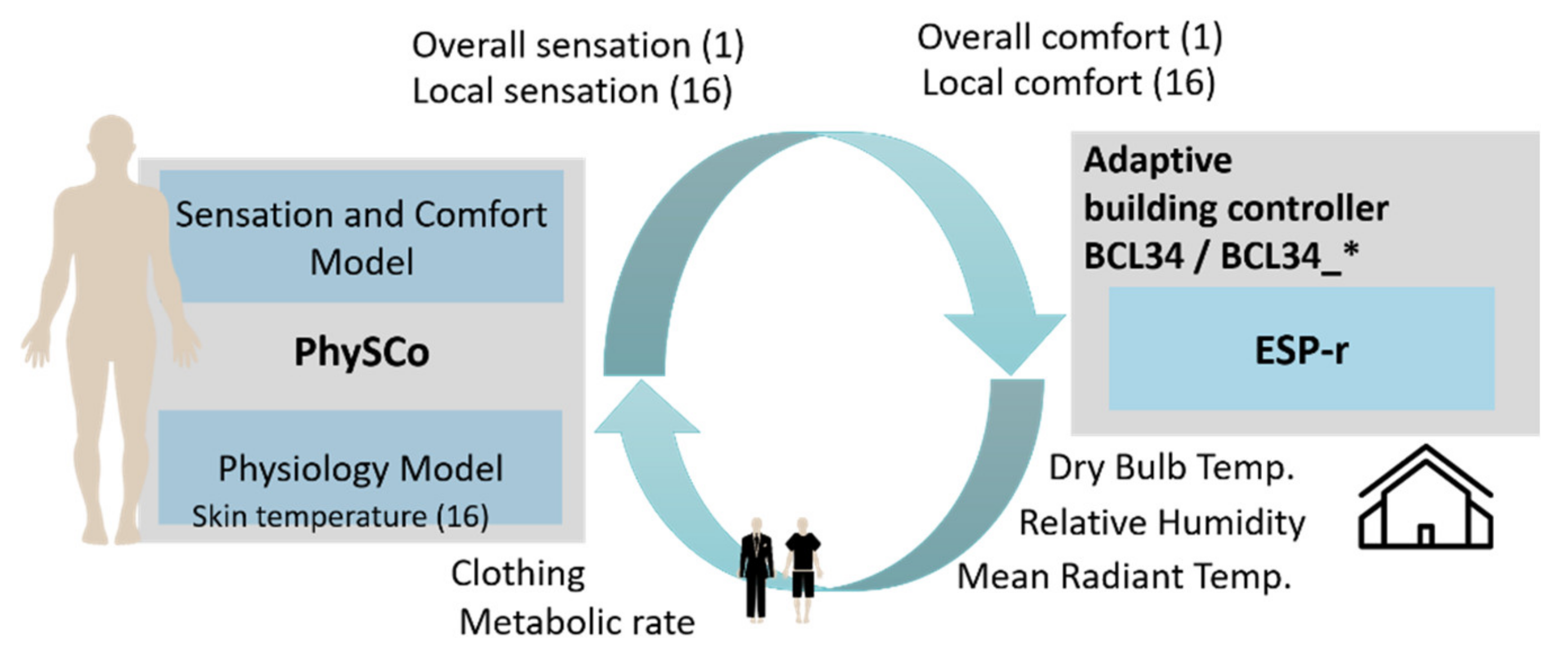
For the planning of decentralized systems and their effect on thermal comfort and, accordingly, to the energy demand of buildings, it is necessary to consider—in addition to the decentralized heating and cooling systems—detailed thermal sensation and comfort values in the building simulation software. An adaptive building controller [
51,
52] was developed within the building simulation software Esp-r [
53] for this purpose. The first step in the development of the adaptive building controller was the coupling of the dynamic PhySCo Model, a “Physiology, Sensation, and Comfort” model, with the building simulation software Esp-r. PhySCo takes transient behavior into account and considers asymmetric conditions. The adaptive controller allows the consideration of decentralized heating and cooling systems and the calculation of detailed sensation and comfort values within the building simulation software [
51].
3. PhySCo (Physiology, Sensation, and Comfort Model)
The PhySCo model can be used as a stand-alone version or for the coupling, which is presented in this article using the building simulation tool ESP-r [
53].
The “Physiology Model” is based on the studies of Stolwijk et al. [
54], Tanabe et al. [
55], Huizenga et al. [
56], and Hoffmann et al. [
57]; the thermal “Sensation and Comfort Model” is based on the equations from Hui Zhang et al. [
22,
48] and Zhao et al. [
58].
The “Physiology Model” uses the values of room temperature, mean radiant temperature, air velocity, relative humidity, and solar radiation, as well as personal parameters such as clothing insulation and activity level (metabolic rate). The model calculates skin and core temperatures for 16 individual body parts under consideration of thermophysiological control mechanisms such as sweating, shivering, as well as vasodilatation and vasoconstriction of the blood vessels. These values are then used to calculate local and overall sensation and comfort values. Within the adaptive building controller, the local and overall sensation and comfort values are used to control the setpoint temperatures of the central heating and cooling system, as well as to regulate the decentralized heating and cooling systems.
Since body temperature increases with increasing activity level and clothing insulation, which in consequence has a significant influence on the thermal sensation [
58], adjustments were made for the “Sensation and Comfort Model” in the form of newly calculated setpoint temperatures (Ts, i, set) for the calculation of thermal sensation [
41].
4. Coupling of PhySCo with Building Simulation Software Esp-r
The basis of this coupling was presented in 2016 by Boudier et al. [
59] and further developed [
21,
51,
52]. To calculate the 16 skin and core temperatures, the “Physiology Model” requires the measured values of the following environmental conditions: mean radiant temperature (MRT), dry bulb temperature (DB), relative humidity (RH), air velocity, and solar radiation (see
Figure 2).
The mean radiant temperature, air temperature, and relative humidity were determined for each timestep in Esp-r (
Figure 2) and are directly used within the “Physiology Model.” The air velocity was taken as a constant value of 0.1 m/s per body part but could be changed according to a time schedule or other environmental changes. Solar radiation was considered in this study only in the context of room temperature and mean radiant temperature. However, it can also be considered and implemented in the framework of the “Physiology Model” of PhySCo [
60].
For air temperature and relative humidity, one value per building zone was applied for all body parts, whereas 16 individual values were considered for each body part for the mean radiant temperature (MRT). Within the building simulation software, PhySCo uses a new approach in order to calculate 16 detailed MRT values of a manikin, which is called “(Wo)Man in Cube” [
21].
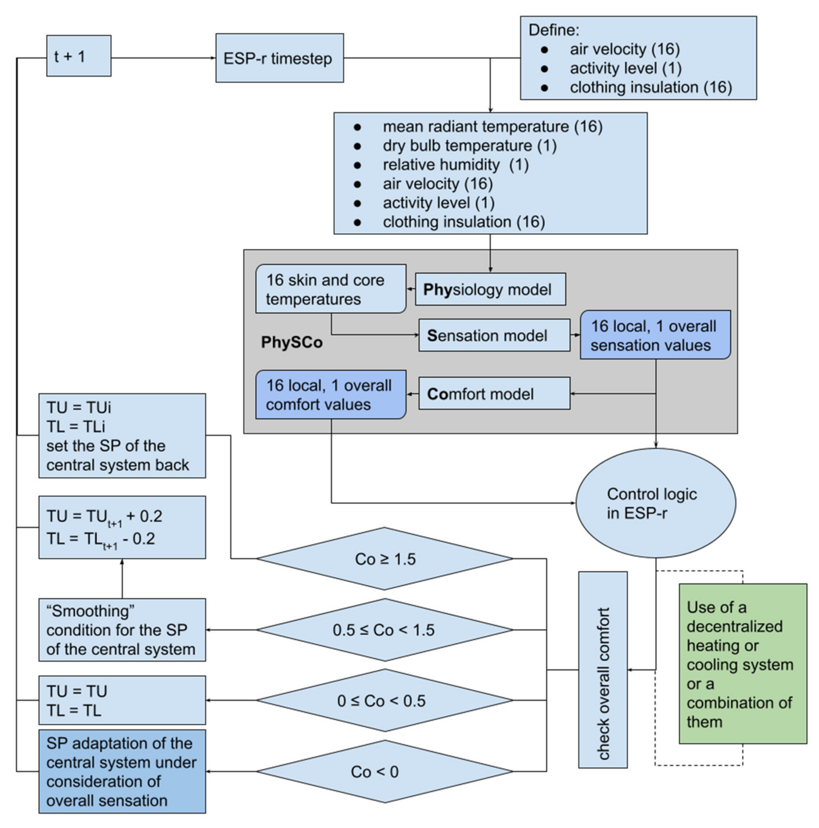
The calculated skin and core temperatures from the “Physiology Model” and the values for thermal sensation and thermal comfort from the “Sensation and Comfort Model” were read into the building simulation software (
Figure 3). The latter were used to adapt the heating and cooling setpoints of the central heating and cooling system. The setpoint adjustment of the adaptive building controller has a direct influence on the indoor conditions and thus on the input values of the “Physiology Model” in the next timestep (
Figure 3).
The “Physiology Model” uses these new environmental conditions to calculate the body’s thermal responses and the 16 skin and core temperatures. These values are then passed to the “Sensation and Comfort Model.” The model calculates the local (16 values) and overall sensation (1 value) as well as the local and overall comfort values for the next timestep (
Figure 3).
The control logic of the adaptive building controller decides according to the values of overall sensation S
o and overall comfort C
o (
Figure 3) to adjust the setpoint of the central heating and cooling system. During the next timestep, the heating and cooling capacity is adjusted accordingly.
In general, the controller can use further adaptive approaches, which are not considered in the presented simulation study to focus purely on the influence of the decentralized systems. The approach, mentioned by Rida and Hoffmann [
61], allows to select a suitable clothing set for the daily outdoor climate and the indoor operative temperature at 6:00 a.m. Furthermore, it considers the overall sensation history of the previous day for the prediction of the clothing model. During the day, the clothing insulation can be adjusted by putting on and taking off other typical clothing items (e.g., a suit jacket) based on the thermal sensation values.
4.1. MRT Calculation with the “(Wo)Man in Cube” Approach
To calculate the mean radiant temperature, the surface temperatures and the view factors were weighted. For a detailed calculation of mean radiant temperature values, it is necessary to use a detailed view factor calculation approach. A view factor defines the percentage of a geometrical view between a person and a surface.
The mean radiant temperature (
) was calculated using the surface temperatures
of the surrounding surfaces (
N) and the view factors
between the surface areas and the manikin with the following equation:
The applied “(Wo)Man in Cube” [
21] approach uses two different view factor calculation methods. It consists of a precalculated set of view factors Vf2 (
Figure 4) and the view factor calculation set Vf1 between the building zone and the MRT sensor boxes. The open-source software View3D [
62] was used first to calculate the view factor set Vf2, which was subsequently implemented in the building simulation software Esp-r. View3D is a verified tool, which is also used within other building simulation software like EnergyPlus [
63]. If the distance between the manikin and the boxes or the pose (standing/sitting) is changed, a new set of view factors must be calculated.
With this method, the view factor set Vf2 stays constant, and the manikin can be randomly moved in the building zone. This approach only requires the calculation of the view factor set Vf1 for each timestep and can deliver accurate MRT values in a short time.
Esp-r uses the individual “surface temperatures” of the MRT boxes and the precalculated view factor file Vf2 to calculate a MRT value per body part. These values are then delivered to the “Physiology Model” within the Esp-r simulation [
51].
4.2. Control Logic for the Adaptive Building Controller
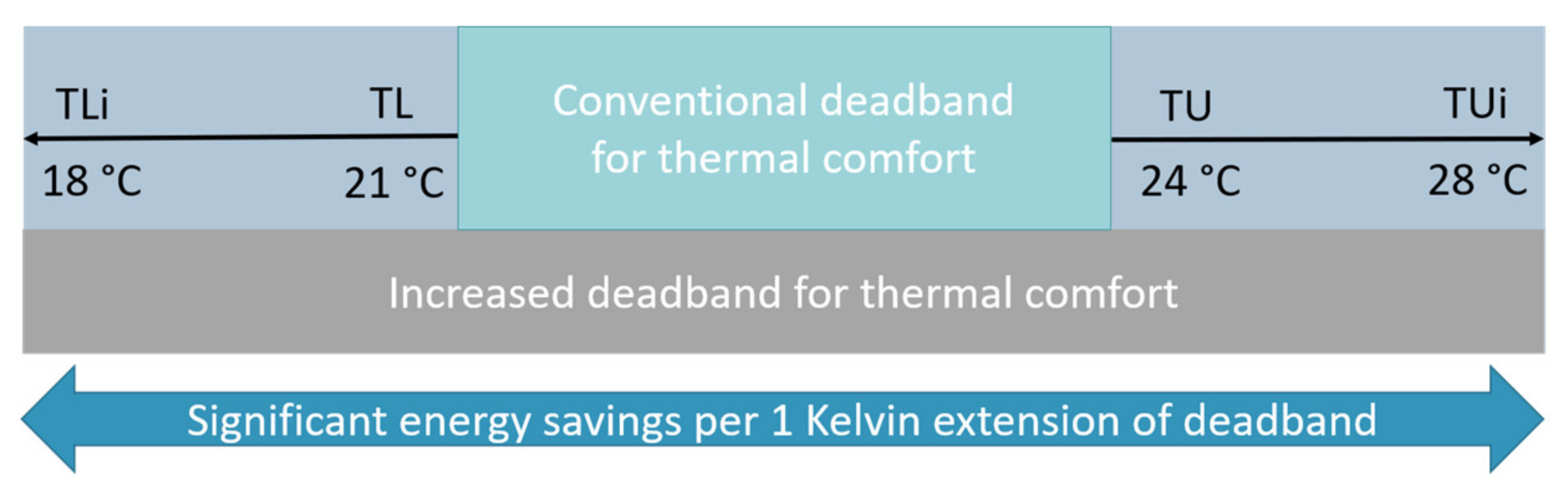
The main goal of the adaptive building controller is to maintain comfortable conditions for the building occupants. At the same time, the controller widens the deadband whenever comfortable conditions are achieved. This reduces the lower setpoint temperature TL (heating setpoint) while increasing (
Figure 5) the upper setpoint temperature TU (cooling setpoint). Initially, the wide deadband is defined with the initial setpoints (TLi, TUi).
The building simulation program Esp-r contains predefined building controllers (BCL) in the main routine (Bcfunc.F). The new controller is assigned the designation BCL34 during the processing and is based on the basic controller BCL00, which takes the area-weighted mean radiation temperature fraction into account. Additionally, the indoor air temperature is included as a convective component. The percentage ratio C between the air temperature θ
a and the mean radiant temperature θ
r can be specified separately for the sensor and the actuator. The mixed sensed temperature θ
s is calculated as follows:
If the sensed temperature
exceeds the upper setpoint TU, heating energy is dissipated (Equation (3)).
represents the heating and cooling demand of the next timestep. If the temperature falls below the lower setpoint temperature TL, heat energy is supplied (Equation (4)).
The adaptive building controller uses the values for overall comfort (Co for “Overall Comfort”) and overall sensation (So for “Overall Sensation”). In the first step, it checks whether 1) the manikin feels comfortable/uncomfortable (
Figure 6) and 2) in case it feels uncomfortable, whether it feels cold/warm (
Figure 7).
If the manikin shows an overall comfort value (Co) greater than 1.5, the setpoints (TU, TL) are reset to the initial setpoints (TUi, TLi) (
Figure 6).
When the comfort value (Co) is between 0.5 to 1.5, the “smoothing” condition applies. This means that the heating and cooling setpoints are slowly returned towards the initial setpoints to save energy when the overall comfort value is within the comfort limits (between 0.5 to 1.5). A setpoint change, which is too fast, is not desired within the above comfort values. The step size to the initial setpoints is 0.2 K per timestep (
Figure 6).
If the manikin just feels slightly comfortable (comfort value between 0 to 0.5), the setpoints remain at their current value from the previous timestep of the simulation (TU = TU, TL = TL) (
Figure 6).
If the overall comfort (C
o) is below zero, it means that the manikin no longer feels comfortable; the overall sensation (So) is checked in the next step, and the setpoints are adapted (
Figure 7).
For example, if the overall comfort value (Co) is less than zero and the overall sensation (So) value is two (manikin feels warm), the upper setpoint TU is gradually decreased until the overall comfort reaches a value above zero (comfortable). If the operative room temperature (To) exceeds the upper setpoint TU, the central heating and cooling system starts and cools down the zone.
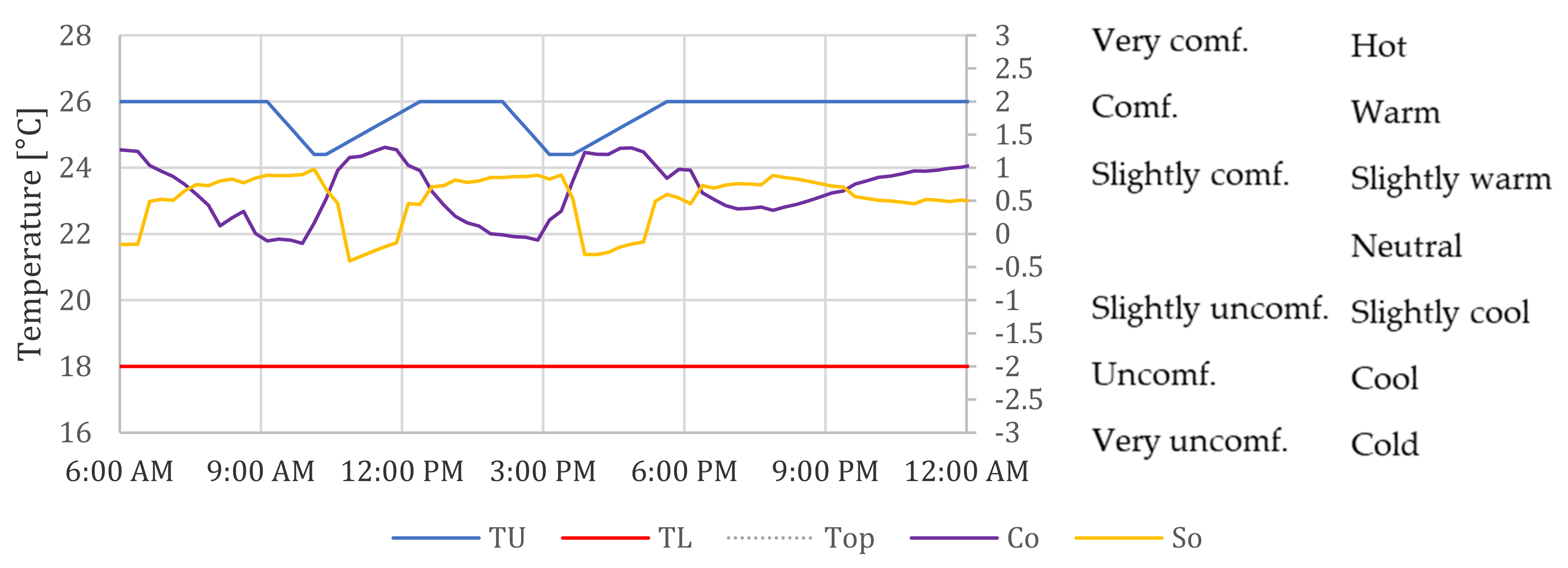
Figure 8 demonstrates a one-day simulation for August, where summer clothing (clo 0.5) was taken into account. Here, an adaptive adjustment of the upper setpoint TU (blue) took place between 9:00 a.m. to 6:00 p.m. The scale of overall sensation (S
o) and overall comfort (C
o) was reduced to the range from −3 to +3.
Around 6:00 a.m., the upper setpoint TU was at the initial setpoint of TUi = 26 °C, and the operative temperature Top was at 25 °C. Overall sensation (So) was in the neutral range at −0.15, and, as a result, the overall comfort value (Co) was in the positive range of 1.2.
During the morning, the So increased and the Co decreased. In the period from 6:00 a.m. to 9:00 a.m., the comfort level was between zero to 0.5, and the setpoints were kept at a constant level. Around 9:00 a.m., Top continued to rise and reached a value of around 26 °C. So reached a value of 0.9, and Co fell below zero. As a result, TU was lowered.
At 10:30 a.m., So dropped again, and subsequently, Co rose. Around 11:30 a.m., the “smoothing condition” became active, as Co was in the range of 0.5 to 1.5. As a result, TU was slowly returned to the initial setpoint TUi of 26 °C. Top rose again, which resulted in an increase in overall sensation (So). Around 2:00 p.m., overall comfort (Co) dropped below zero, and TU decreased again.
During the period from 3:00 p.m. to 4:00 p.m., Co increased continuously and, due to the “smoothing condition,” TU was again shifted towards the initial setpoint of TUi (26 °C). The initial setpoint TUi was reached around 6:00 p.m. and maintained until the end of the day, as the value of overall comfort (Co) ranged from 0.4 to 1.0.
4.3. Control Logic for the Adaptive Building Controller with Decentralized Heating and Cooling Systems
The control logic for the adaptive building controller with the decentralized systems (thermoelectric movable partition, office chair with heating and cooling function, and desk fan) is based on the adaptive control logic (
Figure 6).
The following equation to calculate
[
64] is essential for implementing the decentralized systems. The equation is part of the “Physiology Model”, and it calculates the equivalent temperature
for each of the 16 body parts for every timestep. It considers partially the air temperature
, the radiant temperature
, the air velocity
, and the clothing insulation factor
.
4.3.1. Implementation of the Movable Thermoelectric Wall (ThW)
The movable thermoelectric wall (partition) [
36,
37,
38] was implemented in the building simulation software Esp-r using the “(Wo)Man in Cube” approach [
51]. The thermoelectric wall has three different zones for the three body parts (areas): the head, the upper body, and the lower body, and these zones can be operated independently from each other.
The control logic of the adaptive building controller decides which zone will be used for heating or cooling according to the overall and local sensation values. Through the control logic, the “surface” temperatures of the MRT sensors are overwritten with a defined temperature for heating (35 °C) or cooling (18 °C) purposes.
During the first step the overall sensation value will be checked (
Figure 9). For sensation values greater than 1.0, all three zones will be used for cooling purposes. For sensation values less than −0.5, all zones will be used for heating. If the overall sensation value is in between these thresholds, the local sensation values will be checked (
Table 1).
The sensation values of the responsible body parts (head, arm, and pelvis) were checked. According to the thresholds, the zones of the thermoelectric wall are used for heating or cooling or no climate function is used (
Table 1).
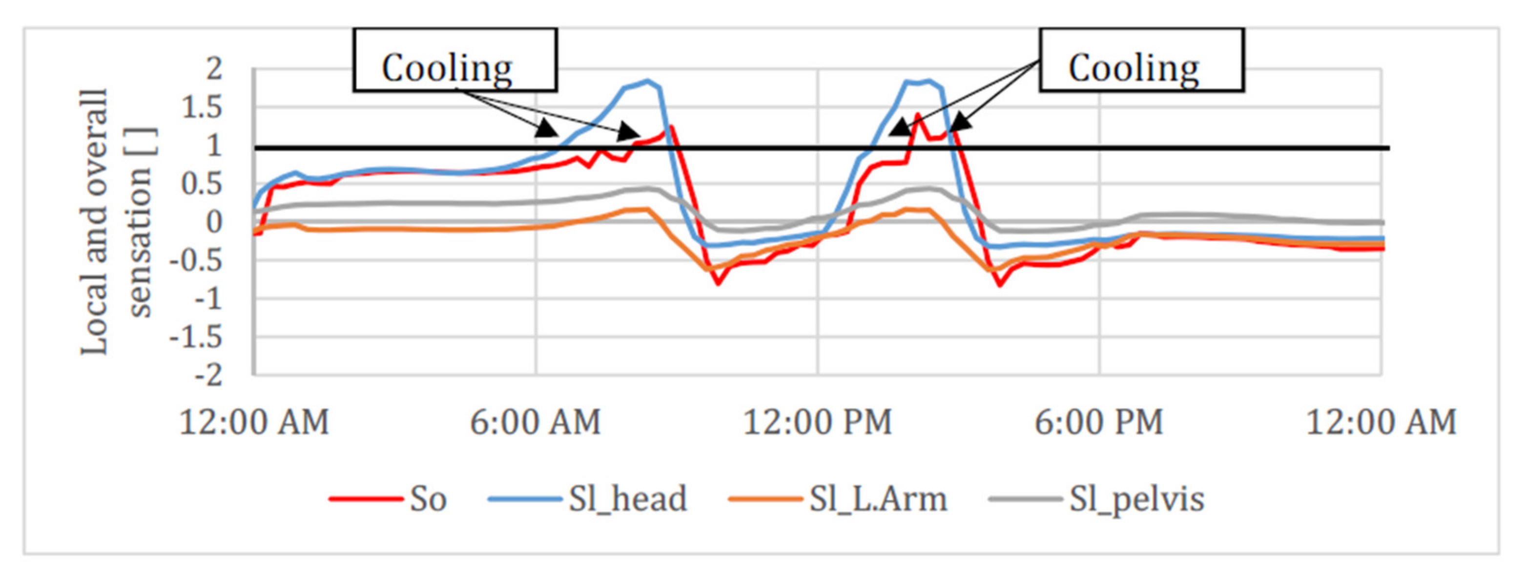
The following charts demonstrate a one-day simulation where the cooling function was used.
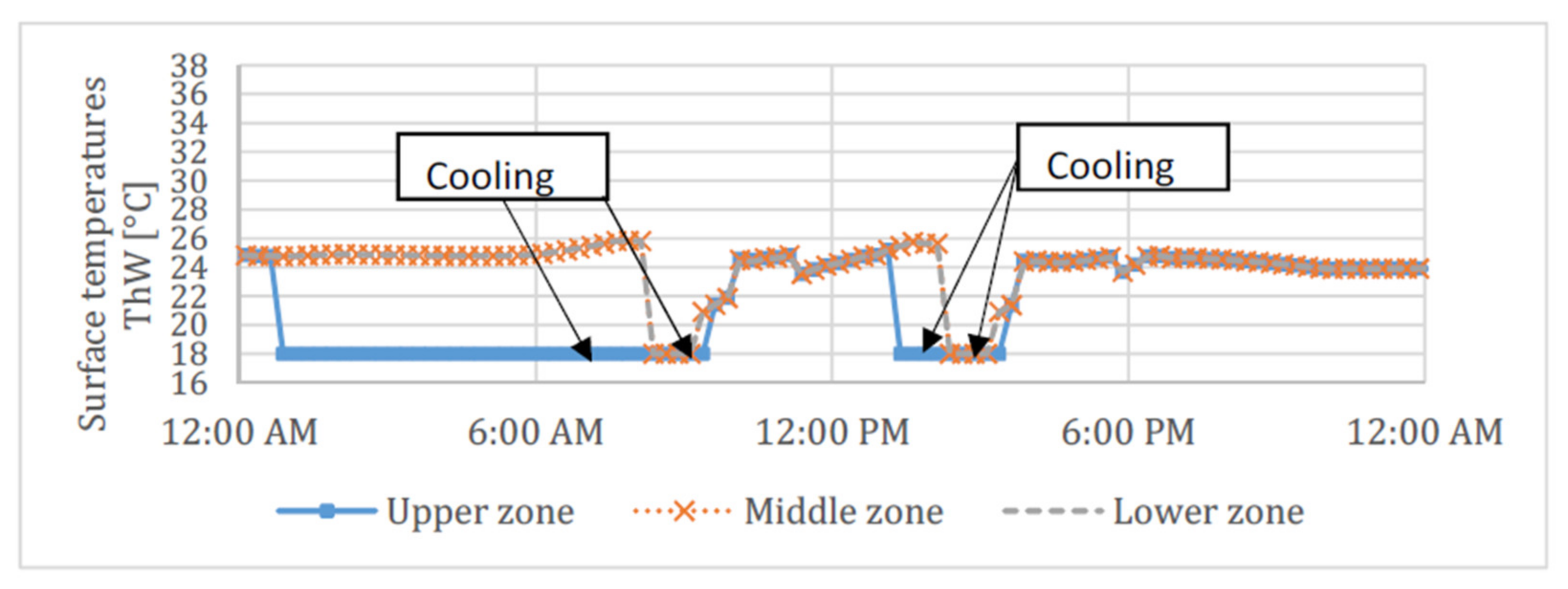
Figure 10 demonstrates the So and Sl values for a one-day simulation in August for Mannheim (Germany), whereas
Figure 11 demonstrates the controlled surface temperatures of the thermoelectric wall accordingly. The threshold of the overall sensation value for controlling the zones of the thermoelectric wall is marked with the black line.
Figure 11 illustrates that the upper zone, which was regulated by the sensation values of the head (Sl_Head), was used for cooling during the night at a constant surface temperature of 18 °C.
In the morning hours, both the local sensation of the head and the overall sensation increased significantly (
Figure 10), which led to the activation of the middle and the lower zones of the thermoelectric movable wall around 8:00 a.m. to start cooling with a surface temperature of 18 °C (
Figure 11). For this, the value of the overall sensation So, which exceeded the limit value of 1 (black line in
Figure 10), was responsible.
Around noon, all sensation values were within the limits of −0.5 to 0.5, so the three zones of the mobile thermoelectric movable wall were overwritten with the current dry bulb temperature. At 1:00 p.m., the local sensation of the head exceeded a value of 0.5 (
Figure 11), so the upper zone of the thermoelectric wall was used for cooling. Later on, the overall sensation exceeded a value of 1, and all three zones were used for cooling.
4.3.2. Implementation of the Office Chair with a Heating and Cooling Function
The second decentralized system within the adaptive building controller is the office chair with a heating and cooling function.
First, in the control logic the overall sensation So (
Figure 12) is checked. If the overall sensation level is greater than 1.0, the chair will be used for cooling. If the overall sensation value is less than −0.6, the chair will be used for heating. If the overall sensation value is in between these thresholds, the chair will not use any of the climate functions, and the chair temperature will be the same as the actual room conditions.
Changes to the surface temperature of the chair have a direct influence on the addressed body parts [
51]. This is expressed with basic Equation (5) for the t
eq of the “Physiology Model,” which will be used for body parts that are not in contact with the chair surfaces. Based on a lab experiment in the Living Lab smart office space in Kaiserslautern, a temperature difference of 4 K can be assumed for the heating and cooling cases. For using the climate functions, the basic equations are adjusted as follows:
Figure 13 demonstrates a one-day simulation with the adaptive building controller and the office chair with a heating and cooling function in January for Mannheim (Germany).
The climate function of the chair backrest and the seat were always used simultaneously and kept at the same surface temperature. The results show that the heating function of the office chair was used because the temperature of the backrest and the seat (ChairTemp_1, ChairTemp_2) increased by 4 Kelvin compared to the dry bulb temperature (DB). If the heating function was not used, the temperature corresponded to the dry bulb temperature (DB). The dry bulb temperature and the chair temperatures are mapped on the left primary axis in the figure.
The threshold value of 0.6 of the overall sensation (So) is shown with the black line. When the overall sensation fell below this limit, the heating function of the chair was switched on. The overall sensation is shown on the secondary axis (right) in the figure.
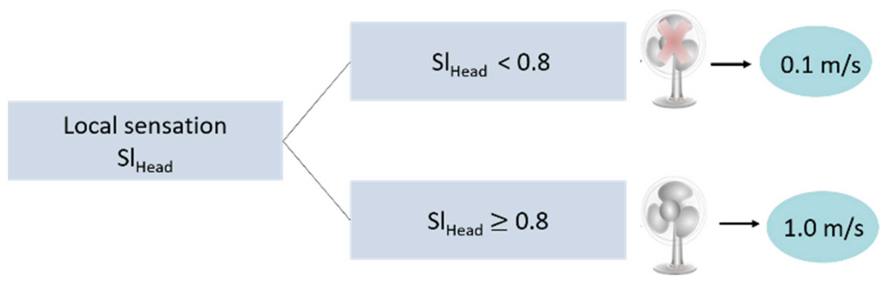
4.3.3. Implementation of a Desk Fan
A desk fan can also be considered in addition to the other decentralized systems. The desk fan is controlled by the local sensation value of the head. If the head sensation value exceeds a value of 0.8 on the sensation scale, the air velocity
increases from 0.1 m/s to 1.0 m/s in Equation (5) for the head in the “Physiology Model” (please see
Figure 14).
5. Simulation Results
The results, building model, and simulation parameters are presented in this section. The simulation results are divided into three parts for winter (15 October to 15 March), spring (15 March to 15 May), and summer (15 May to 15 October). These dates were obtained by considering previous simulations and the resulting clothing sets for these periods.
The results compare the adaptive controller (BCL34) or different combinations of the adaptive controller using decentralized heating and cooling systems (BCL34_*) with the basic controller (BCL00). The following
Table 2 demonstrates the possible combinations of the controller.
5.1. Building Model and Simulation Parameters
The simulations are based on a shoebox model representing an office room with a south-facing window (
Table 3). The “window-to-wall” ratio was 30%. The manikin was located in the center of the room, facing the window. In all cases in which the thermoelectric movable wall was used, it was located on the left side of the manikin.
For the simulations a weather file with temperate climate (Mannheim, Germany) was used. The file provides climate data as hourly values. The data include the outdoor temperature, relative humidity, solar radiation and wind direction and speed [
45].
Internal heat sources considered were a person, a computer and room lighting (
Table 3). The internal loads were constant during day and night and the manikin was located in the room throughout. No mechanical ventilation was taken into account but a 1.5-fold air exchange rate per hour was considered according to DIN 4108-2 for non-residential buildings [
65].
The three interior walls as well as the ceiling and floor were considered to be adiabatic. Thus, neither heat input nor heat loss occurred through these constructions. The U-values for the constructions are shown in
Table 4. The relevant impacts resulted from the outdoor climate and the south-facing exterior wall with the window.
Table 5 shows both the maximum heating and cooling capacity as well as the heating and cooling setpoints. For the adaptive controller, during the winter months for the (then not relevant) cooling setpoint TU higher temperatures and during the summer months for the (then non-relevant) heating setpoint TL, lower temperatures were allowed. The simulations were divided into four simulation periods, during which seasonally adjusted clothing sets were used (
Table 6).
5.2. Winter
5.2.1. Winter Results
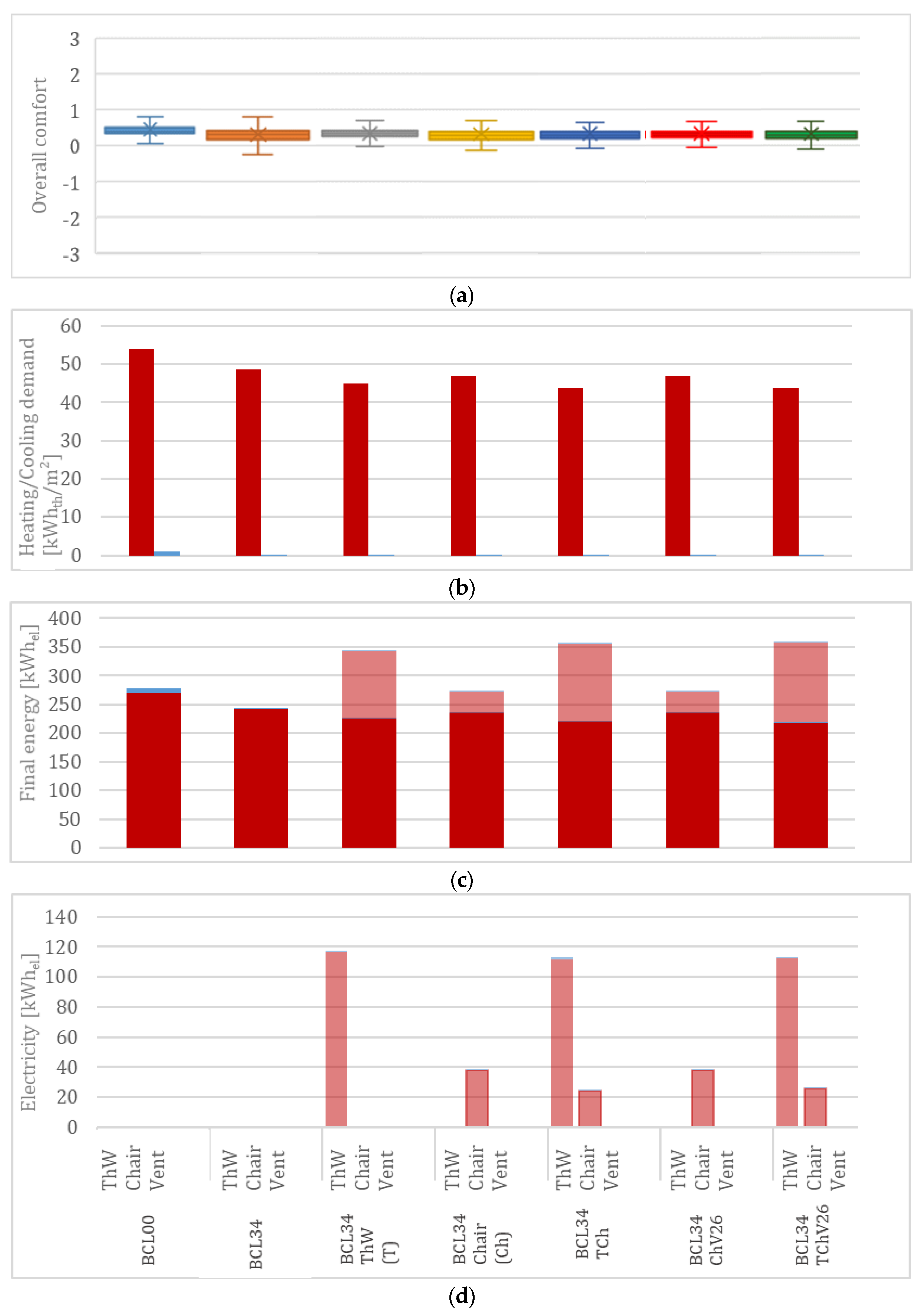
The winter results are shown in the
Figure 15 for (a) overall comfort, (b) heating/cooling demand, (c) the end energy with consideration of the used energy due to the decentralized systems, and (d) the used energy of the decentralized systems.
5.2.2. Overall Comfort
A summary of the comfort values of the controller variations for the winter period is shown in the form of a boxplot diagram in
Figure 15a. For all variations, the achieved peak values of the overall comfort reached a maximum of 1.3. This is due to the control logic: in the comfort range between 0.5 to 1.5, the “smoothing” condition is relevant, which slowly steered the adapted setpoint back towards the initial setpoints (TLi, TUi). If the heating setpoint (TL) or the cooling setpoint (TU) is changed, this has an immediate influence on the calculated comfort.
For better readability, the outliers, i.e., the values that lie above the whisker with 1.5 times the interquartile range, were removed. These outliers could be observed after an increase in the operative temperature Top to above 24 °C and occasionally when the temperature dropped from Top to below 20 °C. This is because the manikin was wearing winter clothing during this period, and it became uncomfortably warm when the temperature rose above 24 °C. Here, the control logic required several timesteps to return the comfort to a positive value. In the variations with decentralized systems, the outliers in the negative range could be reduced compared to the adaptive controller.
For all variations with adaptive building controllers, it can be seen that the median, as well as the interquartile range of the thermal comfort, were slightly below the values of the basic controller. The differences ranged from 0.07 to 0.11 in the median range and from 0.08 to 0.17 in the interquartile range. However, all the variations were predominantly in the positive range.
5.2.3. Heating and Cooling Demand, Used Energy, and End Energy
Figure 15b shows the heating and cooling demand of the different controller variations over the winter period. Additionally, the reduction in the heating demand compared to the basic controller is shown.
Figure 15d shows a comparison of the electricity consumption of the decentralized systems within the controller variations.
From an energy reduction point of view, the use of the adaptive controller variations with the decentralized systems has a positive effect during the winter period. Here, the heating demand could be noticeably reduced for all variations of the adaptive controller with and without decentralized systems. The most significant effects were achieved by the variations BCL34_ThW_Chair_Vent26 and BCL34_ThW_Chair, followed by BCL34_ThW (
Figure 15b). The variations with chair and with chair and fan showed similarly high savings. The adaptive controller can also achieve positive results in terms of heating demand savings compared to the basic controller.
When comparing the power consumption of the decentralized systems (
Figure 15d), it becomes clear that the controller with the thermoelectric movable wall (ThW), in particular, requires a significant amount of energy. This can be explained by its relatively high electrical power demand.
The office chair and the fan showed a very low consumption relative to the thermoelectric movable wall.
This indicates that the variations with thermoelectric heating and cooling wall (BCL34_ThW, BCL34_ThW_Chair, and BCL34_ThW_Chair_Vent26) require more end energy compared to the variations without the thermoelectric movable wall. Although these variations can reduce the heating demand of the central plant, due to the high power consumption of the thermoelectric heating and cooling wall, the end energy demand is not reduced compared to the basic controller (
Figure 15c). The adaptive variations BCL34, BCL34_Chair, as well as BCL34_Chair_Vent26 have a lower energy demand compared to the basic controller.
5.3. Spring
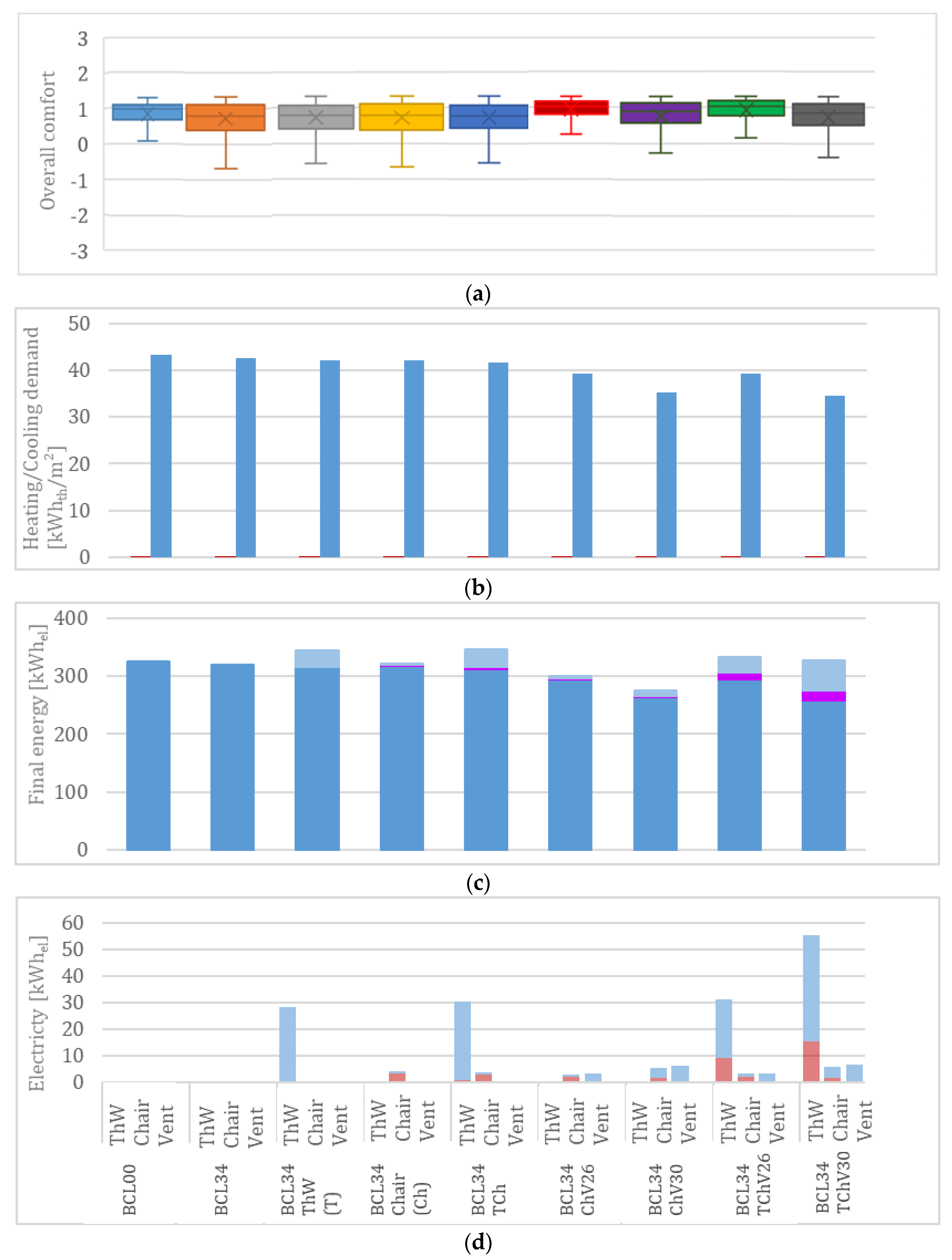
5.3.1. Spring Results
The spring results are shown in
Figure 16 for (a) overall comfort, (b) heating/cooling demand, (c) the end energy with consideration of the used energy due to the decentralized systems, and (d) the used energy of the decentralized systems.
5.3.2. Overall Comfort
It can be seen that during the spring period, the medians as well as the interquartile ranges for the variations with the adaptive building controller were above those of the basic controller (
Figure 16a). The differences varied from 0.24 to 0.47 for the median range and from 0.43 to 0.48 for the interquartile range. While the interquartile range of the basic controller was minimally in the negative range, the interquartile ranges of all variations of the adaptive controller remained in the positive area. The minimum values of the basic controller were above those of the variations. The minimum values of the variations were 0.1 to 0.3 below those of the basic controller (BCL00). The maximum values of all adaptive variations were somewhat above the maximum value of the basic controller of 1.3.
5.3.3. Heating and Cooling Demand, Used Energy, and End Energy
During the spring period, the adaptive controller required a slightly greater cooling demand compared to the basic controller However, all variations could reduce both the heating and the cooling demand. The greatest savings in heating and cooling energy demand were shown by the BCL34_ThW_Chair_Vent30 controller. This is explained by the setpoint adjustment to a higher setpoint of 30 °C (
Figure 16b).
When looking at the electricity consumption of the decentralized systems (
Figure 16d) as well as the end energy (
Figure 16c), it is noticeable that the variations were used differently with respect to the heating and cooling functions. Additionally, during the spring period, the thermoelectric movable wall showed the highest power consumption. It is evident that the power consumption of the thermoelectric movable wall increased further when additional decentralized systems are were (BCL34_ThW_Chair and BCL34_ThW_Chair_Vent). In contrast, the power consumption of the office chair with a heating and cooling function showed either a comparably high power consumption (BCL34_Chair_Vent) or reduced power consumption (BCL34_ThW_Chair and BCL34_ThW_Chair_Vent) for the combined variations with other decentralized systems. Here, the heating function of the chair was reduced if the thermoelectric movable wall was used at the same time.
When the thermoelectric movable wall was used alone, the power consumption was similar for both functions (heating and cooling). When the other decentralized systems were added, the power consumption due to heating predominated. In this case, the thermoelectric movable wall and the chair were used predominantly for heating. These two systems balanced the ventilation of the head and created unequal sensations locally (alliesthesia).
By using the ventilator, the local sensation of the head was affected to such an extent that the thermoelectric movable wall in the upper area was used for heating purposes.
By comparing the end energy consumption, it can be seen that many of the adaptive variations use more end energy than the basic controller. The variations with the thermoelectric movable wall were especially noticeable with a negative impact due to an increased end energy consumption, whereas the variations with the chair stood out positively.
The BCL34_ThW_Chair_Vent variations exhibited the highest consumption. Here, in addition to the heating and the cooling demand of the central system, a significant amount of energy was consumed in heating due to the thermoelectric heating and cooling wall. The end energy demand in relation to the basic controller was thus also the highest (
Figure 16c).
Besides the adaptive controller, the variations with the chair showed the lowest consumption. These variations (BCL34_Chair and BCL34_Chair_Vent26) required only slightly more end energy compared to the basic controller, because of the consideration of the electricity of the chair. The energy consumed by the chair (especially the heating energy) and the fan led to slightly higher consumption but at the same time to higher comfort values.
The variation with the chair and the fan and an increased upper setpoint (BCL34_Chair_Vent30) showed the greatest savings in end energy since both the fan and the chair used relatively little energy, but, at the same time, less cooling energy was used for the central system. Due to the fan, it was possible to increase the upper setpoint up to 30 °C and still offer thermally comfortable conditions. For these temperatures, the heat-sensitive head often dominates the overall comfort level and leads to an uncomfortable state. Maintaining a comfortable state with the fan during these high indoor temperatures helps to reduce the energy demand through the central cooling system. As the desk fan requires low electric power, the effect with the fan regarding comfort and reducing the energy demand is high.
5.4. Summer
5.4.1. Summer Results
The summer results are shown in
Figure 17 for (a) overall comfort, (b) heating/cooling demand, (c) the end energy with consideration of the used energy due to the decentralized systems, and (d) the used energy of the decentralized systems.
5.4.2. Overall Comfort
During the summer period (
Figure 17a), the medians, as well as the interquartile ranges for the adaptive variations (BCL34, BCL34_ThW, BCL34_Chair, BCL34_ThW_Chair, and BCL34S_Chair_Vent30), were below those of the basic controller. The differences ranged from 0.09 to 0.20 for the median and from 0.04 to 0.30 for the interquartile range. On the positive side, it is noticeable that for the two variations with a fan (BCL34_Chair_Vent26 and BCL34_ThW_Chair_Vent26), the median was 0.11, and the interquartile range was 0.28 above those of the basic controller. The variations with the fan and an increased upper setpoint of 30 °C showed similar interquartile ranges, while the median was slightly lower than that of the basic controller.
The increased airflow for the head, which is sensitive to heat, also showed a positive effect in the simulation, as already described in field and laboratory studies [
35,
46,
66,
67]. The comfort values could be optimally increased with the variations BCL34_Chair_Vent26 and BCL34_ThW_Chair_Vent26 compared to all other controller variations. The two variations with the increased setpoint to 30 °C also showed an increase in the interquartile ranges compared to the other adaptive variations and are on par with the comfort values of the basic controller (BCL00).
5.4.3. Heating and Cooling Demand, Used Energy, and End Energy
During the summer period, all adaptive variations reduced the cooling demand compared to the basic controller (
Figure 17b). The adaptive variations with fan showed the greatest reduction in cooling demand compared to the other controllers. The two variations with an increased upper setpoint of 30 °C (BCL34_*30) showed the greatest savings potential compared to the basic controller.
When comparing the end energy required (
Figure 17d), it is clear that the variation that achieved the greatest savings in cooling demand (BCL34_ThW_Chair_Vent30) required the most electricity for the thermoelectric movable wall. The consumption of the movable wall, as well as of the chair and of the fan, increased sharply under these conditions.
It is interesting to note that the thermoelectric heating and cooling wall and the chair require more energy for heating in the variations with the fan. The highest comfort was achieved by different thermal stimuli in this context according to the approach of “Alliesthesia” with the help of the decentralized systems (
Figure 17a). The thermoelectric movable wall was used for heating, while the fan was used for cooling. However, this effect was also obtained when the head was cooled by the fan, which achieved a lower sensation level. Thus, the upper area of the movable wall was used for heating.
Comparing the consumption of the different variations, it is clear that the variations with the chair only required very little power compared to the variations in combination with the thermoelectric wall. The fan requires little energy and is therefore a good solution for the summer months, as it can optimally support the thermoelectric movable wall as well as the office chair.
Figure 17c compares the required end energy of the different variations considering the use of a reversible heat pump in relation to the basic controller. It can be seen once again that the variations with the thermoelectric wall have an increased end energy demand compared to the basic controller and the adaptive controller as well as the other variations with chair. The adaptive variations BCL34, BCL34_Chair, as well as BCL34_Chair_Vent showed reductions compared to the basic controller. As it can be seen in
Figure 17d, the electricity consumption of these decentralized systems turned out to be relatively low and was hardly significant when considering the end energy. The highest reduction compared to the basic controller was achieved with variation BCL34_Chair_Vent30.
6. Discussion
The simulations show that the comfort level can be maintained in a positive range or increased with the help of the decentralized systems while simultaneously reducing the heating and the cooling demand.
Table 7 summarizes the end energy results of the above variations. The achieved reduction is shown with different colors. The limits are defined as follows: dark green (5% to 20%), light green (1% to 5%), and light (0% to −35%). A reversible heat pump was considered to calculate the end energy demand for heating and cooling. Depending on the specific heating and cooling system and the COP values for the reversible heat pump (COP heating = 3, COP cooling = 2), the values for the end energy of the central heating and cooling system may deviate from these results.
With regard to the comfort and the used energy, the adaptive controller, as well as the variations with the chair and with chair and desk fan, can be recommended for all seasons. These variations require somewhat more energy during the spring period, but this is compensated by an increased comfort compared to the basic controller. For this season, the usage of the adaptive clothing model is strongly recommended to show more reasonable results regarding the heating and cooling demand.
During the summer period, the fan should be used in combination with the office chair with a cooling function. The variation with an increased upper setpoint temperature TU of 30 °C significantly saves energy and, at the same time, increases comfort values compared to the basic controller. This setpoint extension to 30 °C regarding the comfort values is only possible with the fan. With the thermoelectric movable wall or the office chair alone, this increase in the comfort values could not be achieved during the summer months. It was possible to increase the comfort using the fan and consequently achieve a reduction in the cooling energy demand. This can be explained by the unique sensitivity of the head to heat influences, which has a significant influence on the overall comfort. In terms of the power consumption of the individual decentralized systems, the fan, as well as the office chair with a heating and cooling function, are much more efficient compared to the thermoelectric heating and cooling wall. That the fan has a greater influence can be explained by the fact that the body is in general more sensitive to the effects of cold influences than to warm ones [
67].
The savings in heating and cooling demand for the adaptive controller with any decentralized heating and cooling variation compared to the adaptive variation demonstrate that the thermal comfort initially increased for all the variations and was kept within the setpoints with the help of the decentralized systems. The adaptation took place in the direction of the initial setpoints, which in turn led to a reduction in the heating and the cooling demand of the central system compared to the adaptive controller.
The results presented here may differ for other building structures and climates. Moreover, the control logic has a strong influence on the comfort and the heating and the cooling demand. In this work, the focus was set on keeping the comfort level in a positive range while at the same time reducing the energy demand of the central heating and cooling system. The results arose from simulations in which comfortable conditions for the manikin were regulated continuously during the day and night, which is the most extreme scenario in terms of energy demand. If only the occupancy hours were considered, the heating and the cooling demand of the centralized system, but also the electricity demand of the decentralized systems, would be noticeably reduced. Furthermore, the activity level could be changed from 1 met to 1.2 met for office activities, according to the recommendations of the standards in this field. This will also influence the heating and the cooling demand. For this study, the focus was set purely on the decentralized systems, but for further studies, the usage of the adaptive clothing model for PhySCo is strongly recommended as this will influence the daily clothing insulation according to the outdoor temperature.
Limitations of the Study
The empirical results reported herein should be considered in the light of some limitations. The decentralized systems are assumed to be used by the occupants for personal conditioning and adjustment of the microclimate. This means that in reality, these systems would not be regulated automatically but controlled by the users themselves. Some scenarios, such as the use of the thermoelectric movable wall for heating while at the same time using the fan for cooling, could occur, but in reality, they would occur less often than shown in the simulations. Although the adaptive controller is useful to estimate the potential for the decentralized systems, it cannot precisely predict the reality.
The results refer to the use by a single person. If several decentralized systems are used, the consumption will increase accordingly. However, due to the different thermal sensitivities of people, the systems may not be used simultaneously. Nevertheless, the utilization of these systems should still be considered in order to create an optimal ambient climate for different room users.
Furthermore, thermal sensation is an individual matter, and certain characteristics could be personalized more in the future. However, it should be considered that the adaptive controller remains for numerical studies. This study used a simple one-zone model as the focus of this research was mainly set on the development of the controller. For further results, a whole building included the detailed HVAC system should be simulated, and ideally an experimental validation with a real building should be performed.
In this study, a thermoregulation model was considered in combination with a sensation and comfort model. These models are sensitive to certain input parameters, which can have a high influence on thermal comfort. The users should be aware of these input parameters and their correlations (e.g, clothing insulation and activity can influence neutral temperatures for thermal sensation).
The adaptive controller used setpoints for the regulation of the central and decentralized heating and cooling systems. So far, this is a pure numerical study, and human subjective studies are missing.
7. Conclusions
In this research work, the effects of different building controllers (a controller with fixed setpoints, an adaptive controller, and variations of the adaptive controller with decentralized systems) were investigated within the simulation software Esp-r with respect to the comfort of a virtual human being as well as to the energy demand of the central heating and cooling system and the end energy under consideration of the decentralized systems.
The simulation results of the adaptive controller, which adapts the setpoints based on the comfort calculation were compared with the results of the basic controller with fixed setpoints. Additionally, the adaptive controller with decentralized systems was tested. The simulation results of the adaptive controller (BCL34) were compared with the results of the following variations with decentralized systems:
The thermoelectric heating and cooling wall (BCL34_ThW),
The office chair with a heating and cooling function (BCL34_Chair),
The two decentralized systems in combination (BCL34_ThW_Chair),
The office chair with a heating and cooling function plus a desk fan (BCL34_Chair_Vent),
The two decentralized systems plus a desk fan (BCL34_ThW_Chair_Vent).
During the winter period, the adaptive building controller achieved a reduction in heating demand for the central heating and cooling system. The comfort values were kept predominantly in the positive range, and an additional reduction in the heating demand was achieved by adding the decentralized systems.
During the spring period, the adaptive controller and all the variations with decentralized systems increased the comfort values compared to the basic controller With regard to the end energy, the variation with the chair (BCL34_Chair) can be recommended since it requires only slightly more end energy with a significant increase in comfort. The cooling demand could be reduced by adding the fan and by increasing the upper cooling setpoint to 30 °C (BCL34_Chair_Vent30).
During the summer simulation period, the adaptive variation with the fan and an upper setpoint of 26 °C achieved the most significant increase in comfort. The adaptive controller (BCL34) and all variations with decentralized systems were able to reduce the cooling demand. When comparing end energy, the variation with the fan and an increased upper setpoint of 30 °C (BCL34_Chair_Vent30) was able to reduce the energy demand the most (15% reduction). With an upper setpoint of 26 °C (BCL34_Chair_Vent26), a reduction of 8% was still achievable.
By implementing a fan in the control logic, it was possible to achieve a further increase in the comfort values during the summer simulation period. This resulted in a substantial reduction of the cooling demand of the central heating and cooling system. It led to a reduction in the cooling demand for the combined variations with the chair and the thermoelectric heating and cooling wall but also to an increased use of the heating function and to higher electricity consumption. In conclusion, the decentralized heating and cooling systems can increase the comfort of the manikin while at the same time reducing the heating and the cooling demand of the central system with the help of the decentralized systems. However, in terms of the total end energy required, not all variations showed a positive balance compared to the reference case of the basic controller. In this work, the variations with a chair and fan were able to achieve a positive effect on comfort and in the reduction of end energy.
It should be mentioned that the actual use of the thermoelectric heating and cooling wall is intended only for the cooling case. The simulations show that especially the heating case requires a significant amount of electrical energy. A further optimization of the control logic is needed in the future.
A virtual building controller, which can represent these systems in an adequate way under consideration of the building occupants, has been missing so far. The approach shown in this article is a promising solution to analyze the potential of decentralized heating and cooling devices as the interest for these decentralized systems is rising after years in research and in the market.
8. Outlook
An important contribution of this work consisted in the modeling of the decentralized systems as separate heating and cooling systems within the plant technology. The decentralized systems should be considered in detail in terms of energy consumption so that more precise conclusions can be drawn regarding the energy efficiency of the overall system with central and decentralized systems in combination. With the adaptive controller, a theoretical potential estimation is possible.
A further step would be the implementation of the virtual adaptive controller in an actual building. Here, different approaches in combination are necessary. First, the thermal sensation and thermal comfort of the occupants must be determined. The aforementioned can be done in different ways. The building occupants can regularly report their subjective sensation and the associated comfort level on a regular basis while operating the decentralized heating and cooling systems in parallel. This approach has already been implemented as a prototype for the thermoelectric heating and cooling wall [
68]. Approximate thermal sensation and comfort can also be determined indirectly via the switch-on rate of the decentralized systems to obtain information about the current conditions (hot/cold). The previous approach has already been implemented for office chairs with heating and cooling functions. Another approach would be the indirect determination of thermal sensation and thermal comfort via the calculation of selected skin temperatures. The determination of skin temperatures could be camera-based [
69] or via sensors, methods that in practice might conflict with privacy or need to be considered as strongly invasive.
At the same time, a comparison with the ambient conditions should be made. For this purpose, the ambient sensors such as, e.g., the Comfort Monitoring Station (CoMoS) could be used. It calculates the PMV value at each individual workplace. When this information is transferred to the building controller, the control of the central system could adjust the heating and cooling capacities accordingly. In addition, it would be possible to create a model-based controller that can respond to predicted weather conditions. In order to respond to the individual preferences of the users, machine learning could be used to determine different profiles for the users.
In order to install such a realistic system, a detailed preliminary planning is required in order to estimate the cost and benefits for thermal comfort as well as possible energy savings. The work presented here provides a solid base for this. The coupled PhySCo model delivers detailed comfort values through annual simulations, which will help to plan the decentralized heating and cooling systems and adjust the central HVAC system in consideration of thermal comfort and the decentralized systems.
The approach shown in this article is a promising solution to analyze the potential of decentralized heating and cooling devices as they are coming more and more to the market.


 ;
;  .
.
 .
.

