Review

A Review on the Estimation of Power Loss Due to Icing in Wind Turbines

by
Leidy Tatiana Contreras Montoya
1,2,*,
Santiago Lain
2 and
Adrian Ilinca
1
1
Wind Energy Research Laboratory (WERL), University of Québec at Rimouski, Rimouski, QC G5L 3A1, Canada
2
PAI+ Group, Energetics & Mechanics Department, Faculty of Engineering, Universidad Autónoma de Occidente, Cali, Valle del Cauca 760030, Colombia
*
Author to whom correspondence should be addressed.
Energies 2022, 15(3), 1083; https://doi.org/10.3390/en15031083
Submission received: 31 December 2021 / Revised: 25 January 2022 / Accepted: 27 January 2022 / Published: 1 February 2022
(This article belongs to the Special Issue State-of-the-Art Energy Related Technologies in Canada 2021-2022)

Abstract

:
The objective of this article is to review the methodologies used in the last 15 years to estimate the power loss in wind turbines due to their exposure to adverse meteorological conditions. Among the methods, the use of computational fluid dynamics (CFD) for the three-dimensional numerical simulation of wind turbines is highlighted, as well as the use of two-dimensional CFD simulation in conjunction with the blade element momentum theory (BEM). In addition, a brief review of other methodologies such as image analysis, deep learning, and forecasting models is also presented. This review constitutes a baseline for new investigations of the icing effects on wind turbines’ power outputs. Furthermore, it contributes to a continuous improvement in power-loss prediction and the better response of icing protection systems.

1. Introduction

In the Nordic countries, where the wind potential is higher, wind production is abundant in winter (the wind is stronger, and the air density is higher) as the power available in the wind varies with the cube of the wind speed. According to the International Energy Agency Wind Technology Collaboration Program Task 19, by 2020, the installed wind power capacity in cold climates was 156 GW and is expected to reach 224 GW in 2025 [1]. However, when blades are covered with ice, the aerodynamic properties change (lift and drag coefficients), and as a result, the power generated is reduced or sometimes ice can stop the turbine [2,3,4,5,6]. Moreover, the ice layer on blades creates an undesirable load, increasing the fatigue of rotor components, and safety hazards from ice that is thrown from the blades [3,4,5,6]. Annual icing losses were estimated to be about 20% of the yearly power output [6,7] and between 20% and 50% in the aerodynamic performance [7]. The best option for maximizing energy production from a turbine operating under icing conditions involves understanding the performance loss that may be predicted during the icing event [5].
Despite the importance of its study, the icing phenomenon has not been fully understood due to its complexity and its dependence on multiple factors such as [8,9,10,11]: Air temperature, humidity, pressure, wind speed, blades’ angle of attack, size of water droplets, blade geometry, point of operation, among others. Until now, there have been no reliable icing predictions systems. However, many models represent rime ice formation on the wind turbine blades, whereas just a few predict glaze ice formation [9].
For years, the estimation of ice accretion impact on wind turbines has been restricted to two dimensions, i.e., the problem has been simplified to an airfoil section of the blade. However, a typical horizontal-axis wind turbine (HAWT) has a twisted blade geometry of, usually, a number of different section forms [12]. This particular blade geometry requires three-dimensional simulations for improved accuracy. However, icing affects not only the blade; it affects the entire wind turbine with various types of 3D effects, such as the effect of flowing air along the radial direction caused by the blades’ rotation [3,6,12]. As demonstrated in reference [13], the flow velocity magnitude in a 3D simulation involves a considerable non-zero component in the z-direction along the blade, which can result in complex fluid–structure interactions and, as a result, a more complicated flow pattern.
Numerical modeling of atmospheric ice accretion on wind turbines is a complex coupled process involving ice shape prediction, airflow simulation, water droplet behavior, boundary layer characteristics, and iced surface thermodynamics with phase changes [4,10]. At present, the models used for the numerical analysis of wind turbine icing have been initially developed for aeronautical applications. For example, in the case of LEWICE, FENSAP-ICE, the Empirical tuned cylinder-based model by Makkonen, and TURBICE [2,14].
This paper focuses on the actual state-of-art of power loss estimation of wind turbines under icing conditions using numerical methods such as CFD (Computational Fluid Dynamics). It provides guidelines to the knowledge needed for modeling the icing phenomenon and examines the numerical techniques used to analyze wind turbine performance. The objective is to present the methods available to quantify wind turbines’ power loss under icing conditions.
The paper is structured as follows: Section 2 summarizes the CFD approach employed in the simulation of ice accretion. Section 3 presents the Blade Element Momentum (BEM) theory for the aerodynamic analysis of wind turbines. Section 4 reviews the academic research oriented towards CFD–BEM and whole 3D CFD approaches. Finally, Section 5 presents the main conclusions and future work.

2. CFD-Based Models for Icing Conditions

The modeling technique attempts to integrate the processes of ice accretion and aerodynamic analysis of the iced object into a single CFD-based icing model. The numerical simulation can be described through integrated thermo–fluid dynamic steps [2,13,15]: (1) fluid flow simulation, (2) droplet behavior, (3) surface thermodynamics, and (4) phase changes. For the last two steps, additional models should be used. All the models will be updated every time step for higher accuracy. In the end, a mesh displacement occurs due to the ice accretion. Thus, updating the multiphase flow solution after every surface boundary displacement guarantees that the solution reflects changes in geometry (see Figure 1).

2.1. Airflow Simulation

The airflow simulation consists of discretization of the governing Partial Differential Equations for conservation of mass (continuity equation—Equation (1)), momentum (Navier–Stokes equation—Equation (2)), and energy (Equation (3)) [10,13].
ρ a t + ρ a U = 0
ρ a U t + ρ a U U = σ i j + ρ a g
ρ a E a t + ρ a U H a = ( κ a T a + ν i τ i j + ρ a g U
where ρ is the air density, and U is the velocity vector. Subscript a refers to the air solution, T refers to the air static temperature in Kelvin, σ i j is the stress tensor, and E and H are the total initial energy and enthalpy, respectively.
The airflow is considered as a turbulent flow; hence, to resolve oscillations and eddies produced in the flow, time-based Navier-Stokes equations and a fine resolution are required. However, these eddies and oscillations become too small as the Reynolds number increase, so the Reynolds-Averaged Navier–Stokes (RANS) approach is more suitable. Based on observations, the RANS formulation averages the velocity variations in the flow field across time [15].
Considering the above, several RANS models and modifications are available depending on its application, and they are based on how the turbulent eddy viscosity is computed. In response to the above, several turbulence models such as k-epsilon, k-omega, Shear-Stress Transition (k-omega SST model), Spalart–Allmaras, and Large Eddy Simulation (LES) have been used. However, four of them have been widely used in flows around airfoils and wind turbines [15].
The Spalart–Allmaras model is a one-equation turbulence model. The one additional equation is used to model the turbulent viscosity transport. Because of its compromise between acceptable computational cost and desired accuracy in turbulent flow simulations, this turbulence model is frequently employed in aerodynamics [15,16]. Furthermore, several scientists have said that this model is the best performing model when simulating ice buildup on electrical cables, wind turbines, and aircraft [17,18].
The k-epsilon model is a two-equation turbulence model that solves the turbulent kinetic energy (k) and the rate of dissipation of kinetic energy (epsilon) assuming a fully turbulent flow, which gives better results for ice accretion simulation [15]. It is very popular due to its low computational cost, and relatively steady, good, and rapid convergence rate [6,15,19]. However, in some cases, it is not adequate in flows with high-pressure gradients [20]. To correct this issue, the RNG k-epsilon model was developed. Based on the renormalization group, this new turbulence model has correction terms for swirling flow, low Reynolds number flow, flow with high-velocity gradients, and also predicts the smallest recirculation zone and the separation point that is closest to the trailing edge [15]. Villalpando et al. [21] studied different turbulence models and concluded that this model was adequate for simulating icing on wind turbines.
The k-omega model is also a two-equation turbulence model. It is used in cases where k-epsilon is not enough and has trouble with convergence as it is more non-linear [22]. It solves the turbulent kinetic energy (k) and the specific rate of dissipation of kinetic energy (omega).
The k-omega SST model is a four-equation model presented by Menter [23]. It is a combination of the standard k-omega and k-epsilon models. It uses both models in different flow regions, activating the k-omega model near the wall and the k-epsilon model away from the surface [15]. This model has been found to be more accurate than other turbulence models [24] because it allows studying the laminar–turbulent transitions of the boundary layer at high angles of attack; handling the recirculation zones, accurately predicting flow separation, and describing the generation of specific vortices at the trailing and leading edges [15].

2.2. Droplet Behavior

The droplets’ behavior can be described by considering the icing phenomenon as a multiphase flow because the icing rate may be affected by a mixture of ice, air, and liquid water [8,25]. The term Multiphase Flow refers to any fluid flow that has more than one phase or component. They are categorized based on the state of the different phases and hence apply to gas/solid, liquid/solid, or gas/liquid flows [26].
With two extensions, the equations of multiphase flows in CFD are basically the same as those of single-phase flows, applied to each fluid in the simulation. To begin, new equations for each fluid’s volume fraction are included. Second, additional terms are introduced in each phase’s transport equation to simulate interphase transfers such as drag, heat transfer, and mass transfer [6,27]. When neglecting gravity and buoyancy, the liquid water droplets present in the air are influenced by its drag and inertia. If drag dominates inertia, the droplets follow the streamline. However, if the inertia dominates, the droplet hits the object (wind turbine). The ratio of inertia to drag depends upon the droplet size, the velocity of the air stream, and the dimensions of the object in question [25].
The equations involved in multiphase (two fluid interaction) computations are [6]:
  • Mass conservation: the continuity equation for phase q can be expressed as
    t ϑ q ρ q + · ϑ q ρ q v q = p = 1 n m ˙ p q m ˙ q p
    where ϑ , ρ and v denote the volume fraction, density, and velocity for phase q , respectively, and m ˙ represents the mass transfer between two phases.
  • Momentum Conservation: The equation of conservation of momentum for phase q can be written as
    t ϑ q ρ q v q + · ϑ q ρ q v q v q = ϑ q p + · τ q = + p = 1 n R ˙ p q m ˙ p q v p q m ˙ q p v q p
    where τ q = is the q th phase stress–strain tensor, R ˙ p q is an interaction force between phases, p is the pressure shared by all phases, and v is the velocity vector.
Different approaches have been developed for the simulation of the disperse phase present in the multiphase flows, mainly Eulerian and Lagrangian. Each one can obtain accurate results, and their use will depend on the type of study, the flow characteristics, and the particle properties [27]. However, the more robust method will carry a higher computational cost, requiring more time to obtain reliable results [15]. For the icing, several software codes have been developed (FENSAP-ICE, LEWICE, TURBICE, and ANSYS-Fluent) and both approaches have been implemented. For instance, FENSAP-ICE works with a Eulerian approach; TURBICE and LEWICE have implemented a Lagrangian technique [28].

2.2.1. Eulerian Multiphase Model

In this model, the dispersed phase, like the continuous phase, is described as a continuous fluid. This approach involves the concept of phasic volume fractions, describing the space occupied by each phase (solid–liquid, gas–liquid, liquid–liquid) [29]. The laws of mass and momentum conservation are satisfied by each phase individually, the properties of each individual dispersed particle or droplet are averaged, and mass transfer between the phases is not assumed [2,14,26,27]. The presence of the dispersed phase has an important turbulent effect on the continuous phase that comes in the form of viscous drag [7]. In the same way, there is a contribution in the lift force, which represents the transverse force due to rotational strain, velocity gradients, or the presence of walls [26].
The droplet drag coefficient could be based on the empirical correlation for the flow around spherical droplets described by Clift et al., 1978 [7,13]:
α t + ϑ U d = 0
ϑ U d t + ρ a U d U d = C D R e d / 24 K   ϑ U U d + ϑ 1 ρ a / ρ d 1 / F r 2 g
where ϑ is the water volume fraction, U d is the droplet velocity, C D is the droplet drag coefficient, R e d is the droplets’ Reynolds number (Equation (8)), K is the inertial parameter (Equation (9)), and F r is the Froude number ( F r = U / g d ).
R e d = ρ a d U U d μ a
K = ρ d d 2 U 18 L μ a
where d is the droplet diameter, U the wind speed, U d the droplet’s speed, μ a the air dynamic viscosity, and L the characteristic length.
To imitate in-cloud icing conditions, the Eulerian Multiphase Flow Model has been used. The droplet solution of this model makes available, in all the computational domains, the velocity, volume fractions, density, and temperature variables for the phases at any time [2,15]. Another advantage is that we can use the same mesh to calculate multiphase flow and predict ice shape [6,15].

2.2.2. Lagrangian Multiphase Model
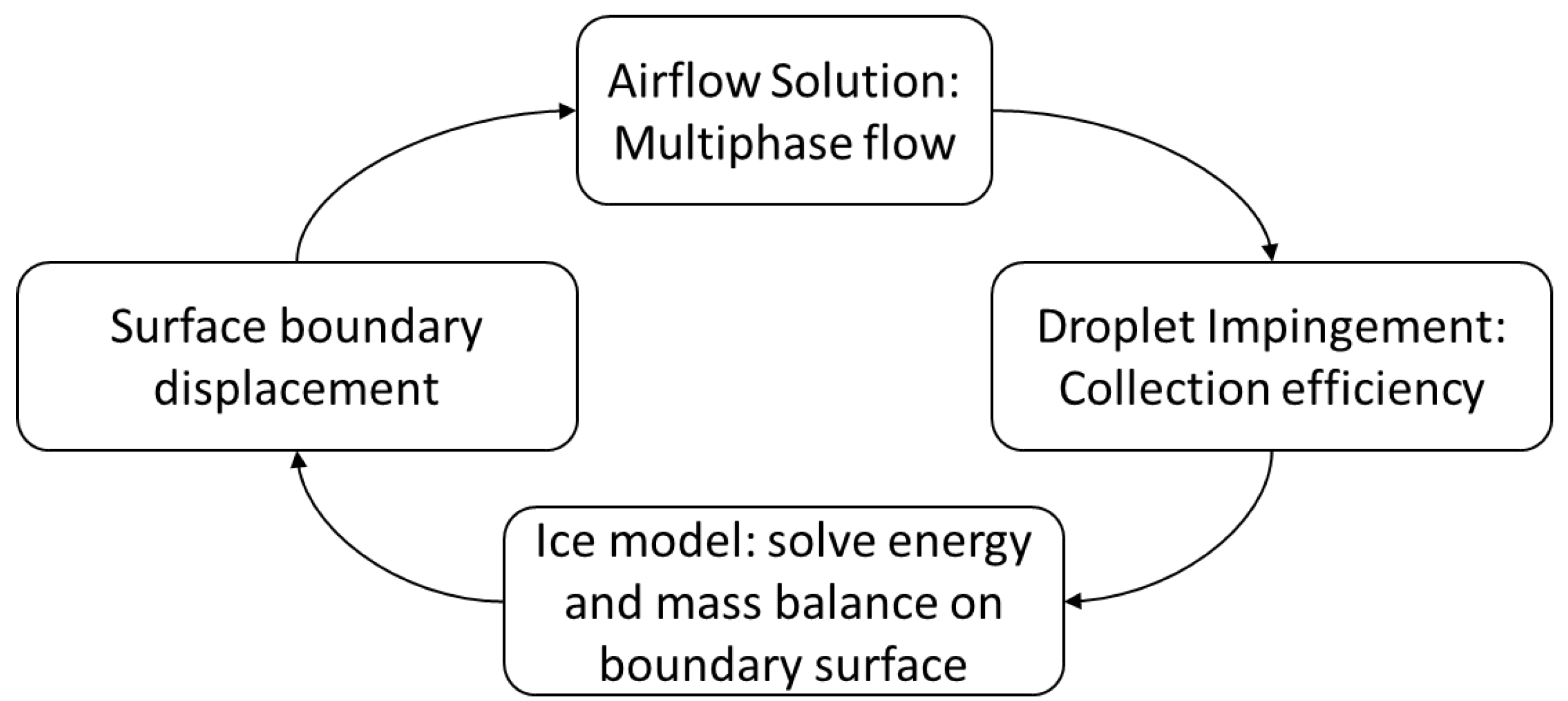
This model solves Newtonian movement equations for each particle or droplet and uses a collision model for handling particle interactions. The calculation of the trajectories of the particles consists of two steps: (1) calculation of the particle motion; and (2) consideration of a particle’s collision with another particle. For the particle motion, Newton’s second law is determined, and the forces acting on each particle, different from collisions, are gravity and the traction force of the fluid phase on the particle [26]. This approach is frequently adopted in 2D icing analysis. The velocities of the water droplets required for icing rate evaluation can be obtained by numerically tracking several water droplets near the icing object. However, tracking enough droplets in 3D to generate the ice layer shape becomes computationally costly [6].

2.3. Ice Accretion

The Ice accretion model involves heat and mass transfer. It is traditionally based on the first-order differential equations of mass conservation and heat transfer developed by Messinger [30] and on the work of Lozowski, Stallabrass, and Hearty [31,32]. Water droplet is simulated as a thin layer of liquid flowing over the blade surface. This film may freeze, vaporize, or sublimate in parts [15]. As a result, the ice accretion model is based on the thermodynamic equilibrium and involves multiple heat fluxes (convective and evaporative cooling, fusion heat, viscous and kinetic heating) [10,13,15]. For the mass conservation, the partial differential equation on solid surfaces will be [7,13]:
ρ f h f t + U f h f = U L W C β m ˙ e v a p m ˙ i c e
where h f is the height of the water film, U f is the velocity of the water film and LWC is the Liquid Water Content. The terms on the right-hand-side represent mass transfer through water droplet impingement (source for the film), evaporation, and ice accretion (sinks for the film). The collection efficiency is represented by β , which is given by Equation (11).
β = ϑ U d · n L W C U
For the conservation of energy, the equation is:
ρ f [ h f c f T ˙ f t + ˙ U f h f c f T ˙ f ] = c f T T ˜ f + U d 2 2 U L W C β L e v a p m ˙ e v a p + L f u s i o n c s T ˜ m ˙ i c e + σ ε T 4 T f 4 c h T ˜ f T ˜ i c e .   r e c + Q a n t i i c i n g
where c f , L e v a p , L f u s i o n , and c s are physical properties of the fluid and the solid, σ is the Boltzmann constant, ε is the solid emissivity, and T ˜ f is the equilibrium temperature at the air/water-film/ice/wall interface.
For the ice accretion calculation, it is common to consider the effect of ice roughness that can reduce energy production by 20% [5,15,33,34], and which also affects the heat transfer [4,15], especially when rime ice is considered [35]. The ice accreted is usually at the leading edge. Still, for icing calculations, the flow solution is computed with roughness set on all the surfaces as droplet impingement, and icing limits are unknown a priori [12]. On this basis, Shin and Berkowitz [36] developed, from empirical data based on experiments, an equivalent sand-grain roughness ( k s ), expressed as a function of the LWC, static air temperature ( T ), airspeed ( U ) and the median volume droplet size (MVD) to determine the ice shapes. With c denoting the airfoil chord and k s / c b a s e = 0.001177 , it is expressed in the following form:
k s = k s / c k s / c b a s e L W C ·     k s / c k s / c b a s e T ·   k s / c k s / c b a s e U ·   k s / c k s / c b a s e M V D ·     k s c b a s e · c
where each sand-grain roughness parameter is given by [36]:
k s / c k s / c b a s e L W C = 0.5714 + 0.2457 L W C + 1.2571 L W C 2   for   LWCs   greater   than   1   g / m 3
k s / c k s / c b a s e T = 0.047 T 11.27
k s / c k s / c b a s e U = 0.4286 + 0.0044139 U
k s / c k s / c b a s e M V D = 1 M V D 20 1.667 0.0333 M V D M V D > 20
Bragg [37] describes in detail a method to correct the drag coefficient due to ice accretion and small-scale surface roughness, which can be expressed by Equations (18) and (19).
Δ C D = 0.01 ( 15.8 × ln k s c + 23.2
C D   i c e d = 1 + Δ C D C D
where k s c can be determined by the method of Shin and Berkowitz [36].

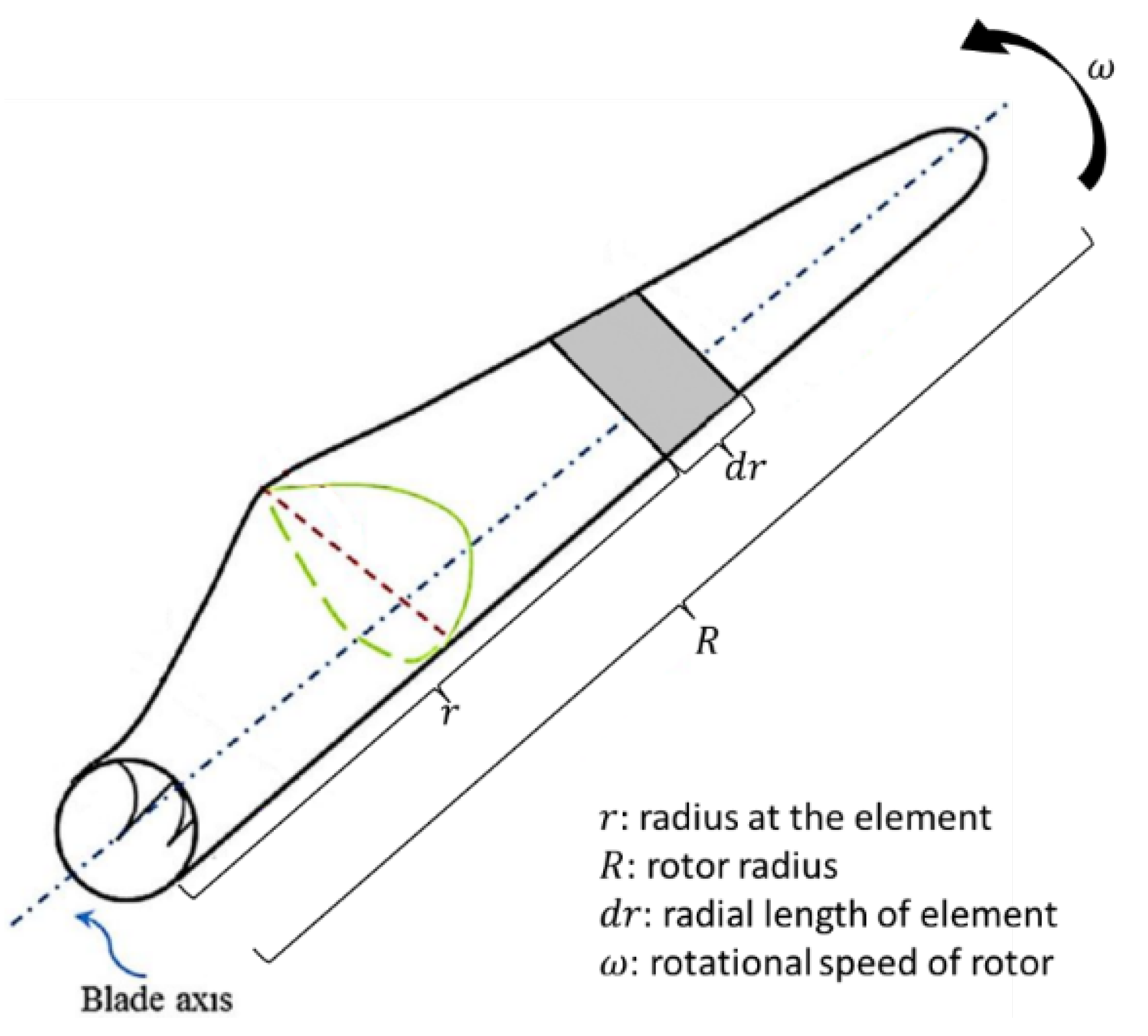
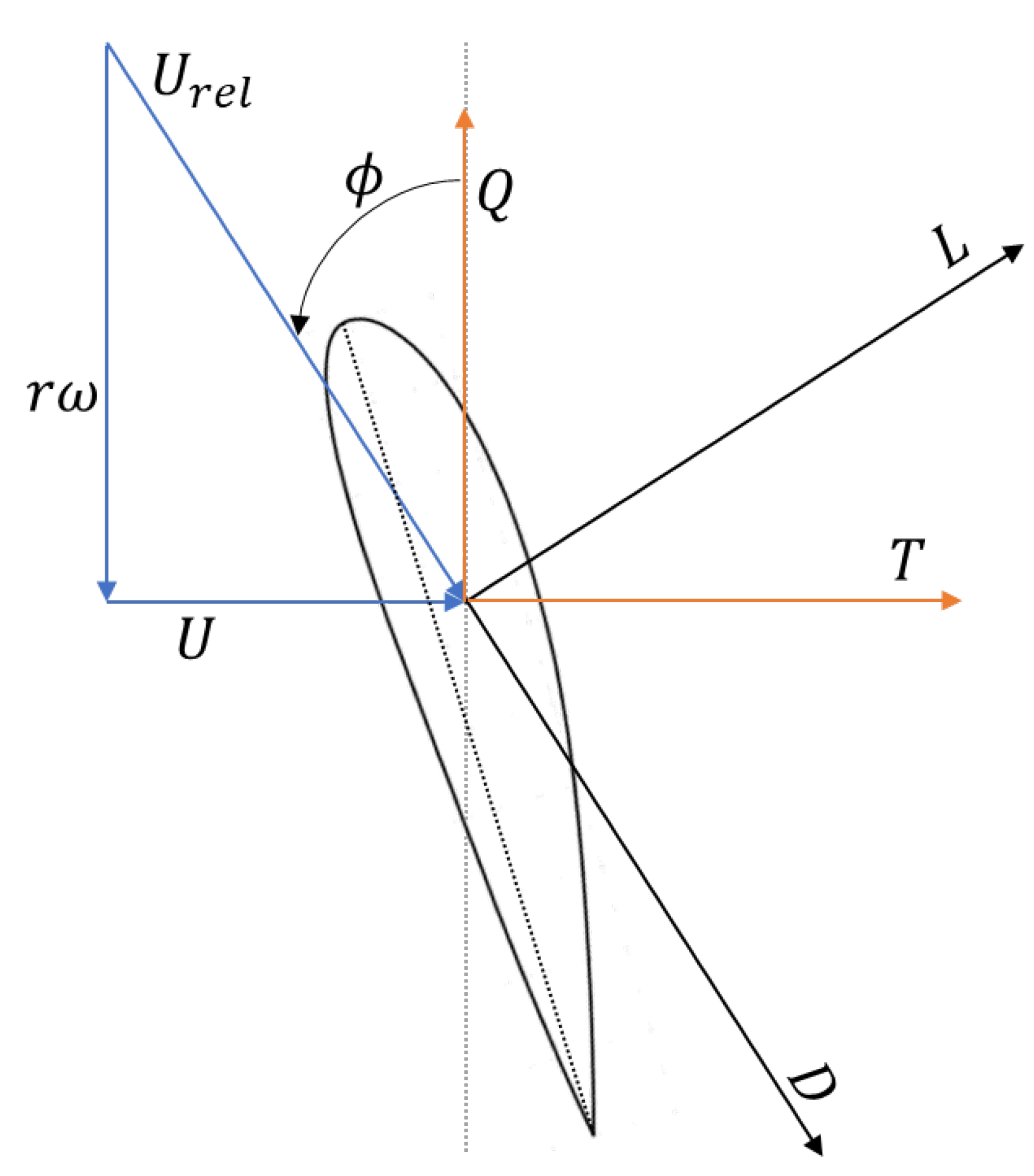
3. Blade Element Momentum (BEM) Theory

Blade Element Momentum Theory (BEM) has become the standard approach for evaluating and designing wind turbines [16]. It combines the momentum theory (analysis of the forces based on the conservation of linear and angular momentum) and the blade element theory (analysis of the forces at a section of the blade based on the blade geometry) [38,39]. It involves dividing the turbine blade into N sections (see Figure 2) applying the following assumptions: (1) there is no aerodynamic interaction between sections; (2) the forces on the blades are determined by the lift and drag characteristics of the airfoil shape using an angle of attack calculated from the incident resultant velocity in the element’s cross-sectional plane; (3) the velocity component in the span-wise direction is ignored; (4) three-dimensional effects are also ignored [38,39,40].
As mentioned before, from the momentum theory, we obtain the thrust (dT) and torque (dQ) on an annular section of the rotor as a function of the axial ( a ) and tangential ( a ) induction factors of the flow conditions [38,39]:
d T = ρ U 2 4 a 1 a π r d r
d Q = 4 a 1 a ρ U ω π r 3 d r
where, U is the air velocity and ω the rotational speed of the rotor.
As for the blade element theory, both forces are also obtained. However, in this case, they are a function of the flow angles at the blades and airfoil characteristics (see Figure 3):
d T = 1 2 B ρ U r e l 2 C l cos ϕ + C d sin ϕ c d r
d Q = 1 2 B ρ U r e l 2 C l sin ϕ C d cos ϕ c r d r
where, B is the number of the blades, c is the airfoil chord, U r e l is the relative wind speed, which is the vector sum of the wind velocity at the rotor ( U 1 a ), and the wind velocity due to rotation of the blade ( ω r 1 + a ), C l is the lift coefficient, C d is the drag coefficient, and ϕ is the angle that the wind speed makes with the plane of rotation.
To determine the complete performance characteristics of a wind turbine requires an iterative solution which consists of initializing a and a to zero, assuming C d = 0 . Drag is excluded from calculating the flow induction factors because drag in attached flows is caused by skin friction and does not affect the pressure drop across the rotor [39,40]. Once the induction factors have been obtained, ϕ , C l and C d are calculated, then the process is repeated until convergence is obtained. With the results for a , a , ϕ , C l and C d , the torque can be calculated by Equations (21) and (23):
d Q = 4 a 1 a ρ U ω π r 3 d r 1 2 B ρ U r e l 2 C l sin ϕ C d cos ϕ c r d r
Finally, the power contribution from each annulus is given by [38,39]:
P = 0 R ω   d Q
and the power coefficient is given by [38,39]:
C P = P P w i n d = r R ω   d Q 1 2 ρ π R 2 U 3
The wind turbine power coefficient depends on the number of blades B , the aerodynamic characteristics of the airfoils, their position r , their pitch angle β , the angle of incidence α , the upstream wind speed U , and the rotational speed ω . The previous velocity triangle (see Figure 3) for an airfoil can be reduced to the relative velocity Urel and the angle of attack α, used as an input parameter for the CFD calculations [39].
The power output of a turbine analyzed using BEM is typically underestimated due to assumption, particularly at low tip speed ratios. Still, the power coefficient tends to be overestimated in high solidity rotors [39,40]. However, span-wise flow exists and is caused by the centrifugal force generated by blade rotation. Therefore, the radial cross-flow is unstable, generating steady and trailing vortices that cause delays in flow separation, drag reduction, lift increase and, eventually, at large angles of attack, lift and drag coefficients that differ significantly from those obtained by 2D computations and measurements [41].
Some corrections have been proposed to this model to improve the calculations and to consider the 3D phenomenon. Some examples are Prandtl’s tip loss factor, Stall–Delay model, Viterna–Corrigan Stall model, and Spera’s Correction.

3.1. Prandtl’s Tip Loss Factor

This factor considers the flow around the blade’s tip from the lower to the upper surface. This flow is due to the different pressure on the blade’s sides, i.e., the suction side has lower pressure than the pressure side, causing lift reduction and thus less power near the tip. The tip loss is more evident in turbines with fewer and wider blades. The correction factor ( F ), introduced into the equations discussed previously, mainly affects the forces derived from momentum theory [39,42].
F = 2 π cos 1 exp B / 2 1 r / R r / R sin ϕ

3.2. Stall–Delay Model

This model takes into consideration the stall–delay phenomenon. The stall region in rotating blades begins in areas with a higher angle of attack. However, the centrifugal force’s effects help reduce the adverse pressure gradient that causes an airfoil to stall. This phenomenon can be described mathematically using laminar boundary layer theory as follows [22,39]:
C l ,   stall = C l + 3 c r 2 Δ C l
C d , stall = C d + 3 c r 2 Δ C d
where, Δ C l and Δ C d are the differences in lift and drag coefficients obtained from the flow with no separation, c / r is the local chord length normalized according to the radial direction. Considering the tip loss and the stall delay, the induction factors can be rewritten as [22,39]:
a = C x σ r 4 F sin 2 ϕ + C x σ r
a = C y σ r 1 a 4 F λ sin 2 ϕ
where C x = C l cos ϕ + C d sin ϕ , C y = C l sin ϕ C d cos ϕ , λ is the tip speed ratio ( λ = ω R / U ), σ r is the chord solidity, defined as the total blade chord length ( c ) at a given radius ( r ) divided by the circumferential length at that radius:
σ r = B 2 π c r

3.3. Viterna–Corrigan Stall Model

This model assumes that a HAWT (Horizontal Axis Wind Turbine) has a high aspect ratio and a flow field that is comparable to that of a 2D airfoil. Consequently, the lifting line theory has been applied to compute the lift coefficient prior to the stall angle of attack. But when the flow enters the fully developed stall zone (angle of attack higher than the angle of attack for which the maximum lift coefficients are observed ( α s )), the Viterna–Corrigan model is used to estimate the aerodynamic coefficients (Equations (33) and (34)) [22,39].
C l = 1 2 C d , m a x sin 2 α + K L cos 2 α sin α
C d = C d ,   m a x sin 2 α + K B cos α
where K L and the K D are:
K L = C l , s C d , m a x sin α s cos α s sin α s cos 2 α s
K D = C d , s C d ,   m a x sin 2 α s cos α s
C l , s and C d , s are, respectively, the lift and drag coefficients at an angle of attack α s of 20⁰ in which C d , m a x depends on the aspect ratio ( A R ), as follows [22,39]:
C d , m a x = 1.11 + 0.018   A R , A R 50 3.01 , A R > 50

3.4. Spera’s Correction

With Spera’s correction, the effect of the turbulent wake is considered using an empirical relation between the angle of attack and the thrust coefficient ( C T ) [22,39]. The correlation is presented in Equation (38):
C T = σ r 1 a 2 C x sin 2 ϕ
If C T > 0.96 , the axial induction factor is:
a = 0.143 + 0.0203 0.6427 ( 0.889 C T )
Whereas, if C T < 0.96 , then the axial induction factor is solved using Equation (30).

4. Estimating Power Loss in Wind Turbines under Icing Conditions

Numerous research studies have been conducted to improve the understanding of ice formation and how ice accretion changes with variations in meteorological parameters. Some examples can be found in references [7,12,13,18,19,43,44,45,46,47,48,49,50,51,52,53,54,55,56,57,58], and the consequences for energy production in [19,50,59,60,61]. Better comprehension and quantification of losses due to icing is crucial for developers and investors in wind farms who have to correctly estimate a project’s expected energy generation to quantify its risks and evaluate its financial viability [50]. As a result, this section gives an overview of the latest research dealing with different methodologies for estimating the power loss due to icing conditions using CFD. Table 1 summarizes the reviewed articles’ atmospheric conditions, simulation setup, and output parameters.

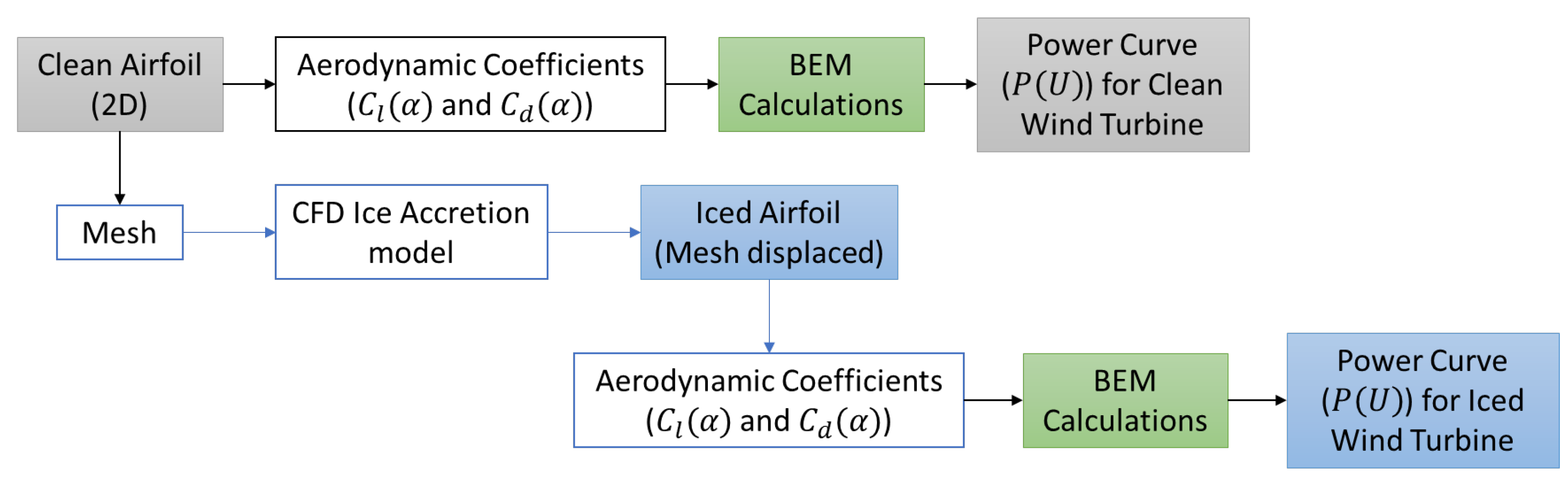
4.1. CFD–BEM Approach

This approach involves both methodologies described in the previous section. Here the CFD is used in two dimensions, more specifically on each section of the blade. The results from the CFD simulation are ice accretion (ice shape, ice mass, ice thickness, among others) and the aerodynamic coefficients (lift and drag). The latter is the input data for the BEM model. A more detailed explanation of the methodology is available in [39]. Figure 4 presents a diagram that visualizes the implementation of this approach.
One of the first studies involving the CFD–BEM methodology was made in 1998 by Jasinski et al. [5]. They carried out a study to estimate the effects of rime ice on horizontal axis wind turbine performance. They predicted four rime ice accretions on the S809 wind turbine airfoil using the LEWICE code to achieve the objective. The icing conditions used were a relative velocity of 65.2 m/s at an angle of attack equal to 5°, an air temperature of −10 °C, an LWC of 0.1 g/m3, 15 and 35 µm for the MVD, and icing event durations of 3 and 7 h. The resulting iced profile combinations were tested in a wind tunnel to obtain the lift, drag, and pitching moment coefficients. Subsequently, the coefficients were used with the PROPID code to predict the effects of rime ice on a 450-kW rated power, 28.7 m diameter, three-bladed turbine operated under both stall-regulated and variable-speed/variable-pitch rotors. For the stall-regulated case, a rotor speed of 48 rpm and a blade pitch of 1.36° were used, while for the variable-speed/variable-pitch case, a tip speed ratio of 7 and the same blade pitch angle were used.
The results obtained by [5] showed performance losses between 14.5% and 20% for the variable-speed/variable-pitch rotor at wind speeds below rated power. A relatively small rime ice profile (0.025 c-long protrusion) produced significantly larger performance losses for the stall-regulated rotor. The rated peak power was surpassed by 16% for a 0.08 c-long rime ice protrusion because, at high angles, the rime ice shape acted like a leading-edge flap, raising the airfoil Clmax and delaying stall. This might result in generator failure and excessive blade loads.
Dimitrova [62] carried out, in 2009, a study to numerically predict the wind turbine energy losses due to light icing conditions. For this purpose, she built the numerical model PROICET, a combination of three software programs (CIRALIMA, XFOIL, and PROPID). The information from a Vestas V80 1.8 MW wind turbine with a NACA63415 airfoil was used to validate the results obtained by the PROICET simulations. The atmospheric conditions were from Murdochville’s site (Quebec), some approximations were made, leading to the following conditions: LWC of 0.05 g/m3, MVD of 20 µm, an airspeed of 8 m/s, temperatures of −6 and −2 °C, and two icing events of 6 and 4 h duration.
The simulations [62] were at five different radial positions on the blade. For each section, CIRALIMA predicted the iced airfoil shape, XFOIL the lift and drag coefficients, and finally, PROPID estimated the wind turbine power curve. The author recommended replacing XFOIL with CFD simulations because it does not give reliable results with large flow separation zones. Despite the high uncertainty, the loss in the lift coefficient was 30%, and the drag coefficient increased by 140%, which was comparable with similar simulations in the literature. The aerodynamic performance deterioration leads to approximately 3.4% power loss. The reduction in the annual energy production of the wind turbine under light icing was estimated at less than 1%. This is due to the light ice conditions assumed (low LWC and the low duration of the event), which led to small ice accumulation on the blades (1.33 kg/m maximum at the blade tip).
Homola and Virk [16] carried out a numerical study of power performance losses on the NREL 5 MW wind turbine’s blade for rime ice conditions. The atmospheric conditions were −10°C, an LWC of 0.22 g/m3, and an MVD of 20 µm. For the CFD calculation, they used a structured-type numerical grid for each section (five in total), a y+ value less than 1, and the roughness height for the iced blade profiles was calculated according to Shin and Berkowitz [36]. The Spalart–Allmaras turbulence model was used. The results obtained [16] showed a gradual increase in the rate and shape of ice accretion when moving from the root section to the tip section of the blade. This is due to a higher water droplet collection efficiency along the blade with an increase in the relative velocity. They also found that the iced turbine presented a significant penalty (27 % of power loss) and that the performance deterioration due to ice is higher with increasing tip speed ratios.
Homola and Virk [16] also evaluated the performance of the wind turbine with the actual turbine controller strategy to identify the operation point for both cases, i.e., a clean and iced rotor. The turbine generator controller was constructed to follow the torque-speed curve calculated by NREL. It consisted of a high tip speed ratio at start-up ( λ = 14 ), which decreases linearly, and then is optimized for maximum power capture by following the torque–speed curve corresponding to a tip speed ratio of 7.55 (wind speed of 10 m/s) for the maximum power coefficient. By crossing the point of the controller curve and the rotor torque–speed curve for both cases, they found out that the operating point for the clean rotor was equal to the designed one. For the iced rotor, the operating point, at the same wind speed, was lower (rotor speed of 1.08 rad/s and λ = 6.80 ) than the optimal value.
To evaluate an improvement for this case evaluated by Homola and Virk [16], the iced rotor data were used to change the turbine controller to adapt to the iced profiles, i.e., instead of operating along the torque–speed curve for the clean blade, the controller maintains the designed tip speed ratio for each wind speed. Homola and Virk [16] shown that modifying the control method may increase the energy capture of an iced turbine by obtaining a power gain for the improved iced case at wind speeds ranging from 7 to 13 m/s.
Turkia and Huttunen [63] developed a method for estimating wind turbine production losses due to icing. Three rime ice cases were simulated with the same meteorological conditions (−7 °C, a wind speed of 7 m/s, an LWC of 0.2 g/m3, and an MVD of 25 µm). Still, the duration of the icing events varies to represent different phases: beginning of icing (19 min), short icing event (3 h), and long icing event (10 h). First, the authors used the code TURBICE to simulate the ice accretion on two blade sections (NACA 64618 airfoil). Then, they used ANSYS FLUENT to model the iced profiles’ aerodynamic properties (lift and drag coefficients). Finally, the power curves for a typical variable-speed pitch-controlled 3 MW wind turbine model and for the same turbine with different ice accretions were generated using FAST software. They also considered the effect of roughness by analyzing the effect of small-scale surface roughness on the drag coefficient using the method described by Shin and Berkowitz [36], and Bragg [37].
As a result, Turkia and Huttunen [63] showed that it is crucial to consider the surface roughness when estimating the aerodynamic penalty caused by icing events, especially for the drag coefficient calculation. The power production drops at the beginning of the icing event due to the accumulated roughness. They also showed a relation between the ice mass and power production. As the mass increases, the power reduction was 18% for the short icing event and 24% for the long one.
Sagol [33] compared both methods previously mentioned to predict ice shape and the corresponding rotor performance. The objective was whether the extra computer resources required by the Full CFD approach are justified by the enhancement in the accuracy of the findings. The 2D and 3D analyses were made in ANSYS FLUENT using the k-omega SST model as turbulence model. Here, the extended Messinger model was used to calculate the ice accretion, and the roughness effect was considered. The reference turbine was the NREL Phase VI. Only one blade was simulated in 3D, adopting a periodic boundary condition and a rotating reference frame technique to account for the blade’s rotation. The icing analyses were performed for a wind speed of 7 m/s, 60 min of ice accretion, an MVD of 20 µm, an LWC of 1 g/m3, and a temperature of −15 °C.
According to the data obtained by [33], the CFD–BEM analysis predicted a 40% power loss, whereas Full CFD anticipated a 25% power loss. This was a foregone conclusion since the ice accumulation on the blade was most substantial when estimated using CFD–BEM. Although the full CFD approach has a substantially higher computational cost, icing assessments in 2D may be inaccurate. Because of the clean blade findings, the authors concluded that the entire CFD procedure offers more accurate results. Finally, using the CFD–BEM method, the ice shape and the related power loss are affected by not taking into account the rotating flow’s 3D features.
Switchenko and Habashi [64] simulated an industrial-scale wind turbine (WindPACT three-bladed 1.5 MW) to demonstrate the impact of atmospheric icing using the CFD–BEM method. The selected icing event was 17 h long and based on data collected at a wind farm located in Gaspé, Quebec, Canada. The FENSAP-ICE model was used for the 2D CFD calculations. The Spalart–Allmaras turbulence model was set up, and for the ice accretion calculation, the authors used the multi-shot strategy available in the software. This strategy enables a quasi-steady simulation of icing events by dividing the overall period of the icing event into shorter intervals, during which ice builds on the blade. Still, until the conclusion of the period, the computational grid is not updated to account for the ice accumulation [64]. To reproduce the data from the wind farm, 34 shots of atmospheric icing were performed. The MVD and LWC were not measured, so three droplet sizes were assumed (20, 50, and 200 µm). As for the LWC, a constant value of 0.1 g/m3 was used. Each shot was divided into 30-min intervals in which the wind speed and temperature were changed according to the on-site information. The impact of surface roughness was also investigated, and three values were selected (1, 3 and 10 mm).
When the authors [64] compared the 2D CFD simulation of the torque for the clean rotor with the 3D CFD simulation, they obtained a good agreement at lower wind speeds with a fully attached flow. Though, with wind speeds higher than 15 m/s, the torque calculated with the 2D approach was underestimated due to larger flow separation regions. Similar behavior was documented by [61]. These discrepancies would impact the simulation of stall-regulated turbines more than pitch-regulated ones.
Regarding the results for the iced rotor, as expected, [64] found more accreted ice at the blade tip than at the blade root. After 17 h, the ice shape at the tip developed a double-horn shape surrounding the stagnation region with a maximum thickness of 21 cm and an ice accretion at the trailing edge. The latter was associated with an increase in the pressure drag. Concerning the effect of roughness, they found that increasing surface roughness will cause an increased shear on the airflow producing a separated region and subsequently lower power outputs; differences of more than 30% were observed. Regarding the influence of droplet size on the power output, [64] found that a larger droplet size resulted in lower power outputs due to increased ice accretion. Finally, Switchenko and Habashi [64] compared the power loss and performance degradation to those measured on-site. A good agreement was found. However, when compared to the average power generated by the wind farm’s turbines, the power produced by the simulated iced turbine was somewhat overpredicted during icing events of between 6 and 15 h.
Etemaddar and Hansen [65] studied the atmospheric ice accumulation on a reference wind turbine blade (NREL 5 MW Virtual wind turbine with NACA 64618 airfoil) and its effect on the aerodynamic performance and structural response. Here, only the results associated with the aerodynamic performance will be presented. The authors evaluated the atmospheric parameters (wind speed, LWC, MVD, and temperature) using the 2D software LEWICE for an icing event with a 24 h duration. Each parameter changed hourly until the 24 h mark was reached. The final iced profile was used as an input in Fluent to estimate the aerodynamic coefficients after icing, and the BEM code WT-Perf was used to quantify the degradation in performance curves (power and thrust coefficients as a function of TSR for four blade-pitch angles of 0°, 5°, 10°, and 15°). It is worth mentioning that the airfoil used corresponded to the outer part of the blade close to the tip.
The domain was discretized with 2D quadrilateral elements for the CFD modeling using an O-Grid topology. The relative wind speed was 50 m/s, the static temperature −7 °C, a roughness height of 0.5 mm was considered, and the k-epsilon model was used as the turbulence model.
The results obtained [65] showed that the power loss was up 35% below the rated wind speed, and the rated power shifted from a wind speed of 11 to 19 m/s. A similar behavior at the operation point was obtained by [16]. Regarding the power coefficient, they found that the difference between clean and iced rotors increases with the TSR for a constant pitch angle. However, for constant TSRs, the difference decreases with an increasing pitch angle. Thanks to these results, the authors concluded that the turbine under icing conditions could continue working at below-rated wind speeds. However, at above-rated wind speeds, the thrust in the iced turbine would be substantially higher than the nominal one, putting the structural components at danger. Hence, they recommend two possible solutions, shut down the wind turbine, or change the cut-out wind speed to a lower value.
In 2016 Yirtici and Tuncer [66] carried out a study to determine the performance losses due to ice accretion on the Aeolos-H 30 kW wind turbine. The 2D ice accretion prediction tool used the Hess–Smith Panel method, the extended Messinger model for the thermodynamic balance, and the Lagrangian approach to obtain the collection efficiency. The effects of splash and break-up were considered. The potential flow solver XFOIL was used to get the aerodynamic loads on each airfoil for the BEM implantation. The predicted ice shapes were validated with experimental and numerical data for two airfoils (NACA 64618 and S809). The results for this first part were in good agreement with those from the literature.
The power loss was analyzed at 11 m/s wind speed and 120 RPM for a selected icing condition (an LWC of 0.05 g/m3, an MVD of 27 µm, temperature of −8 °C, and exposure time of 3 h). The results show [66] that at wind speeds greater than 12 m/s, the XFOIL solution slightly underpredicted the power production compared to experimental data. Finally, the power loss for this icing event corresponded to 24%, which agreed with similar studies.
In 2018, Han and Kim [11] carried out a CFD simulation based on the Dispersed Multiphase Droplet Model (DMP), available in STAR-CCM+, to predict ice formation along the blade-tip of an airfoil’s leading edge. The simulation focused on the rime ice, and the profile analysis was divided into five cases corresponding to planes along the blade. The airfoil chosen was the NACA 64618 from the NREL 5-MW wind turbine. The meteorological conditions were −8 °C, a droplet size of 25 µm, and an LWC of 0.22 g/m3. The authors include the effect of roughness, using the Shin and Berkowitz [36] model, and the Bragg [37] method. The ice accretion was built by updating the mesh deformation for each time step. However, this remeshing process can cause reliability and convergence problems. Thus, they ran a 2D aerodynamic performance simulation utilizing the final iced airfoil shape acquired from the ice accretion simulation. The lift and drag coefficients were estimated for all five cases, and the power calculations were performed using BEM, for this they used the BLADED software. The results showed that ice formation on the blade-tip of the airfoil’s leading edge reduced wind turbine power performance by 8 to 29% at lower-than-rated wind speeds, showing an evident correlation between both parameters. However, at higher-than-rated wind speeds, there was only a little power loss attributable to the blade pitch control system which stabilized the power output. They also found that increasing the angle of attack (AoA) enhanced the rime ice accretion area while decreasing the lift coefficient (significantly at AoA ≥ 8°).
Finally, Han and Kim [11] suggested that an aerodynamic performance control by pitch angle modification is possible at higher-than-rated wind speeds, even if ice has formed on the blade’s leading edge because it will maintain the power steady. Nevertheless, maximum wind turbine efficiency may be reached at lower-than-rated wind speeds by integrating variable-speed operation via generator torque control.
Ebrahimi [68] investigated a small wind turbine’s aerodynamic loads and energy losses (600 kW three-bladed turbine with S816 airfoil blade and 47 m diameter) under wet and dry icing conditions. The wet regime was set up with an MVD of 38.3 µm, an LWC of 0.218 g/m3, −1.4 °C, and an event duration of 360 s. The dry regime was set up with an MVD of 40.5 µm, an LWC of 0.242 g/m3, −5.7 °C, and an event duration of 264 s. The ice accretion simulations were carried out using LEWICE for three-blade cross-sections. The airflow simulations were performed with ANSYS FLUENT, the k-omega SST as the turbulence model, three different wind speeds (9.2, 18.1, and 27.1 m/s), and the production losses were calculated with the BEM theory. For the latter, a tip speed ratio of 7 was chosen.
Regarding the results from [68], in the wet regime, the ice shape (horn shape) accreted on the airfoil had a great influence on the drag coefficient, which became excessively high in comparison to the lift, resulting in rotor stoppage. In the event of a dry regime, performance deteriorated by around 30%.
Zanon and De Gennaro [35] applied the CFD–BEM methodology to predict the performance of a reference turbine (NREL 5 MW) during and after an icing event (8 h), including the possible increase in energy harnessing according to different operational strategies. The ice accretion was computed using ICEAC2D, the airflow analysis was made in ANSYS CFX with the k-omega SST turbulence model, and the BEM code used was WT_Perf. The performance of the wind turbine was determined for a wind velocity of 10 m/s. Two icing conditions were evaluated, rime ice (20 µm, 0.22 g/m3, and −10 °C) and glaze ice (14.36 µm, 0.1605 g/m3, and −2 °C). Three operational strategies were evaluated for the rime ice and only one strategy for the glaze ice.
The first operational strategy controlled the rotational speed by following a precomputed controller torque–speed curve. It allowed the set up of the TSR for the rime ice at 7.68 (IC-1-1) and 7.32 (IC-2-1) for the glaze ice. Therefore, this strategy was considered as the “baseline”. The second operational strategy was the same as that proposed by Homola and Virk [16], which consisted of forcing the optimum TSR (7.55), which was evaluated for the rime ice (IC-1-2). Finally, the third operational strategy was to lower the turbine’s TSR to reduce ice accumulation at the leading edge, so delaying turbine shut-down and conserving the blade aerodynamic performance. It was evaluated for the rime ice only (IC-1-3).
The results [35] showed that during the icing event, the second strategy led to a negligible increase in wind energy (+0.16%). In comparison, the third strategy led to a reduction of wind energy (−8.66%) compared to the baseline. However, following the icing event, the third strategy produced the best performance (+5.8%), while the second strategy gave the worst performance (−3.0%). This finding was contrary to the results presented by Homola and Virk [16], which may be associated with the duration of the icing event considered by each author.
Continuing the research carried out in 2016 by Yirtici and Tuncer [66], Yirtici and Ozgen [69] investigated the ice-induced power losses under different icing conditions on horizontal axis wind turbines. Two turbines were used, the Aeolos-H 30 kW and the NREL 5 MW. The methodology was the same as described in [66], except that in this case, a second tool for the BEM implementation was used: the open-source Navier–Stokes solver, SU2, with the k-omega SST turbulence model.
For the Aeolos-H 30 kW wind turbine, the authors [69] simulated different icing conditions for LWC (0.05, 0.15, and 0.25 g/m3), MVD (18, 27, and 35 µm), temperature (−5, −10, and −15 °C), and time (20, 40, 60, and 80 min) to see the effect on the power production. The operational conditions considered for the turbine were the same as in their previous work [66]. They found that the rime ice forms close to the hub while the glaze ice forms at the blade’s tip. Studying the influence of the MVD and temperature, they found that these parameters do not affect the ice accretion as much as the LWC. The power losses predicted were in the range of 18% to 31%, the maximum value corresponding to the higher LWC and time exposure to the icing event.
For the NREL 5 MW, the authors [69] used the same conditions of Homola and Virk [16], obtaining a 17% power loss, which differs from the 27% in [16]. This discrepancy was associated with the different assumptions made in both studies. For example, [16] neglected the rotational effects and fixed the Reynolds number.
In conditions similar to those in [35], Hildebrandt and Sun [70] conducted, in 2021, a comparative study of two operational strategies in terms of their overall influence on power production. The first strategy was powering through an icing event. In this case, the wind speed was used to determine the airfoil model’s angle of attack and relative airspeed. The second strategy was stopping the turbine during the icing event but resuming the operation after the event. In this case, the rotor speed and the angle of attack were zero. The reference turbine (WindPACT 1.5 MW with a NACA 64618 airfoil) was evaluated for five 2 h icing events with varying atmospheric parameters. The 2D ice accretion was simulated with FENSAP-ICE and concentrated in the outer 30% of the blade. In the droplets module (DROP3D), the authors used the Langmuir D distribution to improve the accuracy of the collection efficiency. In the ice accretion (ICE3D), the small-scale surface roughness was calculated with Shin and Berkowitz’s [36] method, and the multi-shot method was used. The power curves for each icing event were generated using the Xturb-PSU code, which took the aerodynamic coefficients calculated in FENSAP-ICE as input.
The atmospheric parameters were: two wind speeds, 8 and 12 m/s; two temperatures, −8 and −1 °C; two LWC values, 0.2 and 0.48 g/m3; and two MVD values, 30 and 33 µm. When validating the methodology, the authors [70] found that the power curve was underestimated by around 6% in the above-rate wind zone.
In the case of short icing events, suspending the turbines results in a reduction of ice accretion. However, as compared to the method of powering through the event, the impact on power production was smaller. The former was associated with the overpowering effect of surface roughness from ice crystal beading on blade aerodynamics, which occurs whether the blades are rotating or not. Still, for a severe short icing event with below-rated wind speeds, stopping the turbine during the event resulted in a 4.3% improvement in power production.
In summary, the simplicity and numerical stability of the setup are the significant benefits of the CFD–BEM method. However, the negative aspect of 2D CFD simulations is their failure to include information about flow in the blade-span direction. This may be critical as other dynamic phenomena are expected to occur, potentially influencing the results [13]. For example, in [16], the rotational effects on aerodynamic performance were not simplified, resulting in an underestimation of the lift coefficient. Something similar occurs with the BEM model, which can be unreliable in cases where the flow separation zones are important. To conclude, this methodology can generate results with low accuracy, with a tendency to underestimate the aerodynamic coefficients.

4.2. Full CFD Approach

Despite their enhanced accuracy, the adoption of fully CFD-based methods has been far less common; the primary issue is the high CPU requirement involved, which limits an interactive design process. This sub-section presents an overview of recent studies on wind turbines operating under icing conditions using full 3D CFD. Each reviewed contribution briefly defines the computational domain, summarises the essential points of the CFD study, and highlights the principal conclusions obtained.
In 2010, Barber and Wang [50] studied, experimentally and computationally, the icing effects on a three-bladed wind turbine’s performance and aerodynamics. The scale-model wind turbine matched the NREL Phase VI rotor, consisting of two blades with the S809-profile. The icing effects were investigated by attaching simulated and observed ice shapes to the blades. The simulated ice shapes were obtained from the software LEWICE. The parameters used to predict the icing profiles were 44 m for the turbine diameter, 15 rpm rotational speed, a wind speed of 4 m/s, a temperature of −6 °C, an LWC of 0.1 g/m3, an MVD of 35 µm, and an icing duration of 10 h. With these data, six cases were studied: three cases with the same sharp ice shape at the leading edge but varying its span-wise distribution, considering 100%, 25%, and 5% location; two cases with a sawtooth ice shape, one located at the 90% of the span and the other between 80% and 95% of the span; and one extreme ice shape located at the 100% of the span.
The experimental test used a 0.3 m diameter wind turbine model mounted on a carriage moving through a water channel. The turbine’s rotational speed was kept at 800 rpm; by adjusting the carriage velocity between 1.5 and 2.8 m/s, the tip speed ratio (TSR) was wide-ranging from 5 to 8. The experiments were conducted in a water tunnel by the authors [50] since the dynamically-scaled model in their study better replicated the full-scale Reynolds number than a wind tunnel. Though, the measured power coefficient was corrected to consider the Reynolds number difference between the sub-scale model and a full-scale turbine. Barber and Wang [51] used a single blade immersed in a domain comprised of a 120° arc-shape of 4R radius and length for the computational analysis. An unstructured tetrahedral mesh with 10 prism layers on the blade surface was constructed. The Y+ value on the blade surface ranged from 30 to 60. Based on that, the k-epsilon turbulence model with a scalable wall function was selected. The boundary conditions included: velocity a the inlet (1.6–3.1 m/s), outlet pressure, opening constant pressure at the top, free slip at the bottom wall, no-slip wall at the blade, and periodic boundaries with a rotational speed of 800 rpm.
From the experiments, the authors [50] demonstrate that the effect of icing on the power coefficient is higher at high TSRs. This was expected due to losses at high TSRs caused by the blades’ aerodynamic drag, which is altered by the ice shapes. They also found that ice in the last 25% of the span has a significant effect on performance, its impact being greater in the last 5% of the blade’s length, reducing the power coefficient by approximately 29%. They found a major effect on the power coefficient for the extreme ice shape. In this case, no power was generated at TSRs higher than 6, and the power was small for TSRs lower than 6 compared to the other cases. From the Annual Energy Production (AEP) point of view, Barber and Wang [50] considered icing conditions during two months, obtaining an AEP reduction of up to 2%, and 17% in the extreme icing conditions. The CFD simulation results agreed well with experimental data. However, power loss estimated for the extreme conditions was 100%. The analysis of streamlines explained this. In this case, many flow separation zones across the span were observed.
In 2013, Reid and Baruzzi [61] presented a numerical performance degradation analysis of a wind turbine operating under icing conditions using FENSAP-ICE software. They considered NREL Phase VI rotor geometry (two tapered and twisted blades using an S809 airfoil, each 5 m in span). The computational domain consisted of a cylinder with a rotating frame of reference that allowed for steady-state modelling of rotating blades. The turbulence model was the Spalart–Allmaras model. Four icing conditions were evaluated to consider glaze and rime ice. Two wind speeds and temperatures were considered, 7 and 22 m/s, and −3 °C and −15 °C, respectively. The MVD and LWC were constant in all the cases and were 20 µm and 0.5 g/m3, respectively. Three icing periods were considered, which were 10 min, 20 min, and 60 min.
Compared to experimental data in the clean turbine, the FENSAP-ICE calculations slightly overestimated the turbine performance at a wind speed of 12 m/s. in the airflow simulations, this was related with a stall delay, which results in a shorter separation zone and higher torque levels [61]. However, the simulations agreed well with the experimental results for a wind speed of 7 m/s (fully attached flow) and 22 m/s (fully separated flow). Regarding the iced turbine, the authors found that the ice was concentrated at the leading edge in the cases where rime ice was present. In contrast, the glaze ice (higher temperature) allowed the water to run back along the surface in the flow direction, resulting in a larger zone of contamination but with a lower ice thickness.
The authors observed power losses above 50% compared to a clean turbine. The losses are more severe in cases with an icing duration of 60 min, wind speeds between 12 to 15 m/s, and least severe at wind speed above 20 m/s. This was explained by the fact that the ice shape could not expand the area of the separated flow. because of the rime ice shape, which increased flow acceleration at the leading edge, the rime ice conditions caused lower power losses than the glaze ice conditions.
Shu and Liang [67] proposed, in 2017, a 3D ice accretion wind turbine model to simulate glaze ice to study the icing characteristics and output of a small horizontal-axis wind turbine (Twisted blade with a NACA 4409 airfoil along the blade). The simulation was performed according to the icing test conditions using ANSYS FLUENT software. The velocity and collision efficiency were obtained with the Eulerian method and a UDS (User-defined scalar) function. Then, the ice accretion computation was completed in MATLAB based on heat and mass transfer, and GAMBIT was used to create the mesh. In this case, the authors also used one single blade with periodic conditions and a multiple reference frame (MRF) to simulate blade rotation. The standard k-epsilon turbulence model was used. The icing conditions were an LWC of 0.71 g/m3, an MVD of 20 µm, three temperatures (−3, −6, and −8 °C), and three wind speeds (5, 6, and 8 m/s).
The results obtained [67] showed that ice accretion reduces the turbine’s rotation speed and load power. As a result, ice load has a more significant impact on rotor performance than degradation of aerodynamic characteristics. Additionally, as observed in other studies, the ice mass linearly increased from the root to the tip and accumulated at the leading edge. They also found that simulation calculated more severe ice at higher wind speeds and lower temperatures than the test.
Continuing on this topic, Shu and Li [3] carried out, in 2018, a steady-state 3D numerical simulation of a wind turbine rotor using a commercial CFD solver (ANSYS FLUENT) to estimate the blade’s aerodynamic performance after icing. The multiple reference frame (MRF) model, Reynolds Averaged Navier–Stokes equations, and k-omega SST turbulence model were used. The computational domain consisted of two cylinders, the internal domain or rotating zone and the external domain for simulating the environmental conditions or stationary zone. A hybrid mesh was used. The internal domain was unstructured with tetrahedral cells, while for the external domain, a structured grid with hexahedral cells was adopted. The CFD results agreed well agreement with the experimental results for clean and rime-iced rotors within rated-wind-speed, but, overestimated values for glaze-iced rotors at high wind speeds. Under icing conditions, the rotor speed and output power of wind turbines fall drastically as the wind speed increases. The maximum power losses were 63% and 80% at wind speeds ranging from 13 m/s to 14 m/s.
Moreover, the ice effect was smaller on the power coefficient at lower tip speed ratios and became more significant with increases in tip speed ratios (between 26% and 53% for 7 to 8 TSR). Aside from that, ice shapes mostly impact pressure distribution along the leading edge of airfoils, considerably lowering the normal and tangential force at about 62% to 89% radial position. They also discovered that when wind speed increases, the impact of blade icing on pressure distributions and aerodynamic force loss becomes more significant, and that glaze has a greater effect on the aerodynamic force. When influenced by the shape of the ice that is formed, blades are more likely to perform in stall regions at the same wind speed, causing more significant reductions in lift. In addition, flow separation around the frozen blade is more severe at higher wind speeds, resulting in additional momentum and frictional loss, particularly for glaze ice.
It is important to mention that Shu and Li [3] used experimental data to determine the ice shape on each section of the blade profile. The blade geometry was defined for rime and glaze ice conditions based on this information. An irregular horn and protrusion shape characterized the last one. This allowed the reduction of the simulation to an aerodynamic analysis without considering the physics behind the icing phenomenon.
Hu and Zhu [60] simulated the rime ice on the rotating NREL Phase VI stall-regulated turbine. The icing event was treated as a quasi-steady process, and to calculate the rotating airflow, the moving reference frame (MRF) available in ANSYS FLUENT was used. In addition, the k-omega SST model was used as a turbulence model. The authors used the Eulerian method in conjunction with an additional UDS (user-defined scalar) function to estimate the collection efficiency. They used the dynamic mesh technique in ANSYS FLUENT to build the ice shape (see [53] for more information). The icing conditions were: a wind speed of 7 m/s, a rotational speed of 72 RPM, an MVD of 20 µm, an LWC of 1 g/m3, a temperature of −15 °C, and an icing time of 30 min. The boundary conditions were a velocity inlet, a pressure outlet, a periodic surface in the entire domain, and the blade and hub were treated as a moving rotational wall.
Based on the setup described above, Hu and Zhu [60] found that the ice accreted on the blade’s leading edge and that the ice thickness and the ice mass increased along the radial direction. The increase in the ice mass was up to 105%. The power decreased up to 13%, mainly in the outer blade region.
Tabatabaei and Gantasala [59] carried out a study comparing the CFD–BEM method and the Full CFD method. The computation was performed on the full-scale NREL 5 MW rotor (rated wind speed of 11.4 m/s and rotational speed of 12.1 RPM). As a computational domain for the CFD–BEM method, they used a discrete Fourier sine series to approximately replicate an ice shape in the NACA 64618 airfoil from iced profiles available in the literature. In this case, a structured grid was used. The 2D simulations were performed for 15 airfoil sections. Because the rotation of the airfoil was not included in these simulations, the relative velocity to the airfoil was taken into account. For the 3D simulations, the computational domain was a 120° pie-shape, also containing a structured grid with periodic boundaries in the circumferential direction. Two domains were created to account for the rotation, the inner and far-field domains. The software used was ANSYS CFX, and the k-omega shear stress transport (SST) model was used as a turbulence model.
The total power calculated by the CFD–BEM method and the Full CFD for the clean rotor was in close agreement. However, the total power was underestimated by 28% for the iced rotor by the CFD–BEM method. In conclusion, the power coefficient loss due to the ice was 32%, the thrust coefficient was reduced by 11%, and when the ice horn height exceeded 8% of the chord length, the power loss became more significant.
Finally, for the Full CFD methodology, it is important to point out that, to date, the analyses have been carried out in a quasi-steady state. Therefore, uncertainty remains as to how the behavior of the coupling phenomenon would be if analyzed from a transient point of view. Furthermore, the studies have been limited to a single rotating blade, assuming that ice accumulates in the same way on all the blades. It would be interesting to know if this assumption is correct or if there is a difference that could affect the power generated by the turbine.

4.3. Alternative Methods

In 2014, Lamraoui and Fortin [71] proposed a new method based on a rotating helicopter blade analogy. In this study, the authors [71] located the glaze and rime ice on the wind turbine blade (a V80-1.8 MW Vestas, with a diameter of 80 m, a rated wind speed of 14 m/s, a minimum wind speed of 4 m/s, a rotational speed of 16 RPM, a variable pitch angle, and a NACA 63415 airfoil) and detected the critical zones involved in significant power loss. For this purpose, they used the results obtained experimentally for a helicopter’s blade [72]. This approach introduced two concepts: The freezing fraction and the power loss factor. The freezing fraction indicates how rapidly freezing occurs when super-cooled water strikes a solid body; if equal to 1 it reflects complete freezing of liquid water and, therefore, is associated with rime ice. From [72], the critical freezing fraction for a helicopter was estimated as 0.88, which corresponds to a double horn ice shape, which is characteristic of glaze ice.
On the other hand, the power loss factor reflects the normalized changes in power needs for rotor blade helicopters under icing conditions. In case of ice accumulation, the helicopter’s rotor requires more power to sustain the rotation frequency, contrary to the normal operation of a wind turbine, where they reduce the expected power generation. To determine the power coefficient under icing conditions, the power coefficient for clean wind turbine blades was divided by the power loss factor. It is important to mention that this method does not consider the evaporation and sublimation of liquid water masses when calculating the ice mass’ rate of accumulation.
Although the operation of a helicopter rotor and a wind turbine rotor is different, this approach allowed us to find the parameters that maintain the freezing fraction [71]. An MVD of 18 µm, different temperatures (−2.6, −4.5, −12, and −20 °C) and an LWC (0.04, 0.03, 0.2, and 0.36 g/m3) were evaluated. From this evaluation, the parameter that maintains the freezing fraction equal to 0.88, and consequently maximum power loss, was an LWC of 0.2 g/m3, a temperature of −12 °C, and the location was between the 93% and 96% of the blade’ radius. At this point, the power loss was estimated at approximately 40%. Compared with a temperature of −13.5 °C (rime ice along the entire blade), the power loss was slightly lower. As a result, even little temperature changes might cause a change in power loss.
Finally, [71] found that the maximum mass rate and thickness of ice were located at 70% of the blade’s radius and showed a strong dependence with LWC; higher values of LWC resulted in higher accumulations of ice and a shorter required icing duration to reach higher power loss values. Power degradation was regulated by ice thickness when considering the entire blade, independent of the type of ice.

5. Conclusions

The power losses are observed as soon as the icing conditions start. Consequently, annual production losses will depend on the intensity, duration, and frequency of the icing events. This literature review summarizes that both the CFD–BEM and Full CFD methodologies estimated power losses of between 8% and 30%. However, some discrepancies were observed, which could be associated with the assumptions made in the CFD–BEM methodology and demonstrate the importance of considering the complex flow around the iced airfoil in three dimensions. Table 2 summarizes the advantages and disadvantages of the methodologies addressed in the document.
Simulation is an important verification tool that is not as expensive as the experimental tests and allows the study of multiple scenarios. However, one of the difficulties associated with the Full CFD simulations is the high computational cost. This review shows that most studies were carried out only on one blade or in blade sections, not for the entire turbine. Furthermore, some assumptions were made in the analysis: periodic conditions at the boundaries; and that the turbine’s blades behave the same way regardless of their position. Another issue is highlighted in [33,59], as a lack of experimental data under real icing conditions makes it difficult to validate the accuracy of CFD solutions. Currently, the validation is carried out for the aerodynamic analysis in ice-free conditions for which experimental data are available.
One factor that influences the CFD simulation process is the type of accreted ice. Most of the studies presented here concentrate on rime ice. It allows the assumption that the water droplets hitting the blade surface freeze immediately due to rapid heat dissipation, thus leading to ice accumulation. However, the problem becomes more complex with glaze ice, as in this case, it will involve an ice layer and a water film on the blade surface.
Most airflow simulations used the Spalart–Allmaras turbulence model due to its efficiency and low computational cost. However, when simulating in three dimensions (Full CFD), this model lacks accuracy when computing the stall phenomenon.
Likewise, the power loss will also be affected depending on the type of ice. For example, in the case of rime ice, most of the losses are due to an increase in the drag coefficient. However, glaze ice is less studied due to its complexity and differences in the literature between numerical prediction and experimental data. Thus, for the latter, its effect has not been widely documented.
Most of the BEM codes that are available use drag and lift coefficients versus angle of attack as input data. In all simulations, an extrapolation of these coefficients was performed as the calculations concentrated on angles of attack between 0° and 15°. However, the BEM model requires a more extensive range (±180°) to be considered. Therefore, some extrapolations were performed by hand, by comparing similar curves obtained in the literature [63]. At the same time, other authors used models or modifications such as the Tagler model [11] or the Viterna extrapolation method [33,65].
None of the simulations considered ice break-up or shedding. It was assumed that all the accumulated ice remained on the blade during the entire icing event. In reality, this does not happen, as some ice fragments can detach due to the turbine’s rotation. Therefore, when validating the results of the simulations with actual data, it is essential to take these factors into account.
The simulations were carried out in a stationary or quasi-stationary state, which also generates an inaccuracy in the calculations since the icing phenomenon and the operation of the turbines are transitory processes.
Currently, no sensors correctly measure LWC and MVD, which are fundamental parameters for numerical simulations. This unavailability of information also leads to significant uncertainty regarding the computationally generated results since we resort to the use of empirical correlations or reusing values explored by other authors.
Ice growth was calculated only in the last 30–40% of the blade since it has been estimated that this is the part of the blade that most influences turbine performance.
To conclude, progress has been made in the application of CFD to understand the icing phenomenon and its effect on wind turbines’ performance. However, there is still work to be done, for example, to simulate the complete turbine, making use of a transient methodology such as “sliding mesh”, which is available in Ansys, to predict the ice growth on each blade of the wind turbine and estimate its performance as a whole. This could help to better understand how the icing affects the wind turbine and not only the blade’s profile.

Author Contributions

Conceptualization, L.T.C.M. and S.L.; methodology, L.T.C.M.; formal analysis, L.T.C.M.; investigation, L.T.C.M.; writing—original draft preparation, L.T.C.M.; writing—review and editing, S.L. and A.I.; supervision, S.L. and A.I. All authors have read and agreed to the published version of the manuscript.

Funding

This research received no external funding.

Institutional Review Board Statement

Not applicable.

Informed Consent Statement

Not applicable.

Conflicts of Interest

The authors declare no conflict of interest.

References

  1. IEA Wind TCP TASK. Task 19 Report 2020: Wind Energy in Cold Climates; VTT Technical Research Centre: Espoo, Finland, 2020. [Google Scholar]
  2. Pedersen, M.C.; Sørensen, H. Towards a CFD Model for Prediction of Wind Turbine Power Losses due to Icing in Cold Climate. In Proceedings of the 16th International Symposium on Transport Phenomena and Dynamics of Rotating Machinery, Honolulu, HI, USA, 10–15 April 2016; p. 6. [Google Scholar]
  3. Shu, L.; Li, H.; Hu, Q.; Jiang, X.; Qiu, G.; He, G.; Liu, Y. 3D numerical simulation of aerodynamic performance of iced contaminated wind turbine rotors. Cold Reg. Sci. Technol. 2018, 148, 50–62. [Google Scholar] [CrossRef]
  4. Makkonen, L.; Laakso, T.; Marjaniemi, M.; Finstad, K.J. Modelling and Prevention of Ice Accretion on Wind Turbines. Wind Eng. 2001, 25, 3–21. [Google Scholar] [CrossRef]
  5. Jasinski, W.J.; Noe, S.C.; Selig, M.S.; Bragg, M.B. Wind Turbine Performance Under Icing Conditions. J. Sol. Energy Eng. 1998, 120, 60–65. [Google Scholar] [CrossRef]
  6. Fu, P.; Farzaneh, M. A CFD approach for modeling the rime-ice accretion process on a horizontal-axis wind turbine. J. Wind Eng. Ind. Aerodyn. 2010, 98, 181–188. [Google Scholar] [CrossRef]
  7. Jin, J.Y.; Virk, M.S. Study of ice accretion along symmetric and asymmetric airfoils. J. Wind Eng. Ind. Aerodyn. 2018, 179, 240–249. [Google Scholar] [CrossRef]
  8. Makkonen, L. Models for the growth of rime, glaze, icicles and wet snow on structures. Philos. Trans. R. Soc. London. Ser. A Math. Phys. Eng. Sci. 2000, 358, 2913–2939. [Google Scholar] [CrossRef]
  9. Zimnickas, V.; Gecevičius, G.; Markevičius, A. A Literature Review of Wind Turbines Icing Problems. In Proceedings of the 13th International Conference of Young Scientists on Energy Issues—CYSENI 2016, Kaunas, Lithuania, 26–27 May 2016; pp. 109–115. [Google Scholar]
  10. Virk, M.; Mughal, U.; Hu, Q.; Jiang, X. Multiphysics Based Numerical Study of Atmospheric Ice Accretion on a Full Scale Horizontal Axis Wind Turbine Blade. Int. J. Multiphysics 2016, 10, 237–246. [Google Scholar] [CrossRef] [Green Version]
  11. Han, W.; Kim, J.; Kim, B. Study on correlation between wind turbine performance and ice accretion along a blade tip airfoil using CFD. J. Renew. Sustain. Energy 2018, 10, 023306. [Google Scholar] [CrossRef]
  12. Abbadi, M.; Mussa, I.; Lin, Y.; Wang, J. Preliminary Analysis of Ice Accretion Prediction on Wind Turbine Blades. In Proceedings of the AIAA Scitech 2020 Forum, Orlando, FL, USA, 6–10 January 2020. [Google Scholar]
  13. Jin, J.Y.; Virk, M.S.; Hu, Q.; Jiang, X. Study of Ice Accretion on Horizontal Axis Wind Turbine Blade Using 2D and 3D Numerical Approach. IEEE Access 2020, 8, 166236–166245. [Google Scholar] [CrossRef]
  14. Pedersen, M.C.; Yin, C. Preliminary Modelling Study of Ice Accretion on Wind Turbines. Energy Procedia 2014, 61, 258–261. [Google Scholar] [CrossRef] [Green Version]
  15. Martini, F.; Contreras Montoya, L.T.; Ilinca, A. Review of Wind Turbine Icing Modelling Approaches. Energies 2021, 14, 5207. [Google Scholar] [CrossRef]
  16. Homola, M.C.; Virk, M.S.; Nicklasson, P.J.; Sundsbø, P.A. Performance losses due to ice accretion for a 5 MW wind turbine. Wind Energy 2012, 15, 379–389. [Google Scholar] [CrossRef]
  17. Hudecz, A.; Koss, H.; Laver, M.O. Ice Accretion on Wind Turbine Blades. In Proceedings of the 15th International Workshop on Atmospheric Icing of Structures (IWAIS XV), St. John’s, NL, Canada, 8–13 September 2013; p. 8. [Google Scholar]
  18. Makkonen, L.; Zhang, J.; Karlsson, T.; Tiihonen, M. Modelling the growth of large rime ice accretions. Cold Reg. Sci. Technol. 2018, 151, 133–137. [Google Scholar] [CrossRef]
  19. Homola, M.C.; Virk, M.S.; Wallenius, T.; Nicklasson, P.J.; Sundsbø, P.A. Effect of atmospheric temperature and droplet size variation on ice accretion of wind turbine blades. J. Wind. Eng. Ind. Aerodyn. 2010, 98, 724–729. [Google Scholar] [CrossRef]
  20. Taborda Ceballos, M.A. Simulación Tridimensional Transitoria de Flujo Turbulento en Configuraciones de Interés Industrial. Master’s Thesis, Universidad Autónoma de Occidente, Cali, Colombia, 2015. [Google Scholar]
  21. Villalpando, F.; Reggio, M.; Ilinca, A. Assessment of Turbulence Models for Flow Simulation around a Wind Turbine Airfoil. Model. Simul. Eng. 2011, 2011, 714146. [Google Scholar] [CrossRef] [Green Version]
  22. Bai, C.-J.; Wang, W.-C. Review of computational and experimental approaches to analysis of aerodynamic performance in horizontal-axis wind turbines (HAWTs). Renew. Sustain. Energy Rev. 2016, 63, 506–519. [Google Scholar] [CrossRef]
  23. Menter, F. Zonal Two Equation k-w Turbulence Models For Aerodynamic Flows. In Proceedings of the 23rd Fluid Dynamics Plasmadynamics, and Lasers Conference, Orlando, FL, USA, 6–9 July 1993. [Google Scholar]
  24. Sagol, E.; Reggio, M.; Ilinca, A. Assessment of Two-Equation Turbulence Models and Validation of the Performance Characteristics of an Experimental Wind Turbine by CFD. ISRN Mech. Eng. 2012, 2012, 428671. [Google Scholar] [CrossRef]
  25. Virk, M.; Homola, M.; Nicklasson, P.J. Atmospheric icing on large wind turbine blades. Int. J. Energy Environ. 2012, 3, 1–8. [Google Scholar]
  26. van Wachem, B.G.M.; Almstedt, A.E. Methods for multiphase computational fluid dynamics. Chem. Eng. J. 2003, 96, 81–98. [Google Scholar] [CrossRef]
  27. ANSYS Inc. Multiphase Flows Models and Capabilities. Available online: https://www.ansys.com/products/fluids/multiphase-flows/multiphase-flows-models (accessed on 18 August 2020).
  28. Ayabakan, S. TURBICE-The Turbine Blade Icing Model, and its further development via a new interface. In Proceedings of the Winterwind International Wind Energy Conference, Ostersund, Sweden, 12–13 February 2013. [Google Scholar]
  29. Laín, S.; Aliod, R. Study on the Eulerian dispersed phase equations in non-uniform turbulent two-phase flows: Discussion and comparison with experiments. Int. J. Heat Fluid Flow 2000, 21, 374–380. [Google Scholar] [CrossRef]
  30. Messinger, B.L. Equilibrium Temperature of an Unheated Icing Surface as a Function of Air Speed. J. Aeronaut. Sci. 1953, 20, 29–42. [Google Scholar] [CrossRef]
  31. Lozowski, E.P.; Stallabrass, J.R.; Hearty, P.F. The Icing of an Unheated, Nonrotating Cylinder. Part I: A Simulation Model. J. Appl. Meteorol. Climatol. 1983, 22, 2053–2062. [Google Scholar] [CrossRef] [Green Version]
  32. Lozowski, E.P.; Stallabrass, J.R.; Hearty, P.F. The Icing of an Unheated, Nonrotating Cylinder. Part II. Icing Wind Tunnel Experiments. J. Appl. Meteorol. Climatol. 1983, 22, 2063–2074. [Google Scholar] [CrossRef] [Green Version]
  33. Sagol, E. Three Dimensional Numerical Prediction of Icing Related Power and Energy Losses on a Wind Turbine. Ph.D. Thesis, École Polytechnique de Montréal, Montréal, QC, Canada, 2014; p. 177. [Google Scholar]
  34. Blasco, P.; Palacios, J.; Schmitz, S. Effect of icing roughness on wind turbine power production. Wind Energy 2017, 20, 601–617. [Google Scholar] [CrossRef]
  35. Zanon, A.; De Gennaro, M.; Kühnelt, H. Wind energy harnessing of the NREL 5 MW reference wind turbine in icing conditions under different operational strategies. Renew. Energy 2018, 115, 760–772. [Google Scholar] [CrossRef]
  36. Shin, J.; Berkowitz, B.; Chen, H.; Cebeci, T. Prediction of ice shapes and their effect on airfoil performance. In Proceedings of the 29th Aerospace Sciences Meeting, Reno, NV, USA, 7–10 January 1991; p. 264. [Google Scholar]
  37. Bragg, M.B. Rime Ice Accretion and Its Effect on Airfoil Performance. Ph.D. Dissertation, The Ohio State University, Columbus, OH, USA, 1982; p. 180. [Google Scholar]
  38. Manwell, J.F.; McGowan, J.G.; Rogers, A.L. Wind Energy Explained: Theory, Design and Application, 2nd ed.; Wiley: Hoboken, NJ, USA, 2010. [Google Scholar]
  39. Martini, F.; Contreras, L.T.; Ilinca, A.; Awada, A. Review of Studios on the CFD-BEM Approach for Estimating Power Losses of Iced-Up Wind Turbines. Int. J. Adv. Res. 2021, 9, 633–652. [Google Scholar] [CrossRef]
  40. Burton, T.; Jenkins, N.; Sharpe, D.; Bossanyi, E. Aerodynamics of Horizontal Axis Wind Turbines. In Wind Energy Handbook; Wiley: Hoboken, NJ, USA, 2011; pp. 39–136. [Google Scholar]
  41. Laín, S.; Contreras, L.T.; López, O. A review on computational fluid dynamics modeling and simulation of horizontal axis hydrokinetic turbines. J. Braz. Soc. Mech. Sci. Eng. 2019, 41, 375. [Google Scholar] [CrossRef]
  42. Martínez, J.; Bernabini, L.; Probst, O.; Rodríguez, C. An improved BEM model for the power curve prediction of stall-regulated wind turbines. Wind Energy 2005, 8, 385–402. [Google Scholar] [CrossRef]
  43. Li, Y.; Sun, C.; Jiang, Y.; Yi, X.; Zhang, Y. Effect of liquid water content on blade icing shape of horizontal axis wind turbine by numerical simulation. Therm. Sci. 2019, 23, 1637–1645. [Google Scholar] [CrossRef] [Green Version]
  44. Li, Y.; Sun, C.; Jiang, Y.; Yi, X.; Xu, Z.; Guo, W. Temperature effect on icing distribution near blade tip of large-scale horizontal-axis wind turbine by numerical simulation. Adv. Mech. Eng. 2018, 10. [Google Scholar] [CrossRef]
  45. Li, Y.; Sun, C.; Jiang, Y.; Yi, X.; Guo, W.; Wang, S.; Feng, F. Ambient Temperature Effect on Wind Turbine Blade Icing Shape by Numerical Simulation. In Proceedings of the 2nd International Conference on Industrial Aerodynamics (ICIA 2017), Qingdao, China, 18–20 October 2017; pp. 290–297. [Google Scholar]
  46. Pallarol, J.G.; Sunden, B.; Wu, Z. On Ice Accretion for Wind Turbines and Influence of Some Parameters. In Aerodynamics of Wind Turbines; WIT Press: Southampton, UK, 2014; Volume 81, pp. 129–159. [Google Scholar]
  47. Virk, M.S.; Homola, M.C.; Nicklasson, P.J. Relation Between Angle of Attack and Atmospheric Ice Accretion on Large Wind Turbine’s Blade. Wind Eng. 2010, 34, 607–614. [Google Scholar] [CrossRef]
  48. Virk, M.S.; Homola, M.C.; Nicklasson, P.J. Effect of rime ice accretion on aerodynamic characteristics of wind turbine blade profiles. Wind Eng. 2010, 34, 207–218. [Google Scholar] [CrossRef]
  49. Homola, M.C.; Wallenius, T.; Makkonen, L.; Nicklasson, P.J.; Sundsbø, P.A. The relationship between chord length and rime icing on wind turbines. Wind Energy 2010, 13, 627–632. [Google Scholar] [CrossRef]
  50. Barber, S.; Wang, Y.; Jafari, S.; Chokani, N.; Abhari, R.S. The Effect of Icing on Wind Turbine Performance and Aerodynamics. In Proceedings of the European Wind Energy Conference (EWEC), Warsaw, Poland, 20–23 April 2010; p. 11. [Google Scholar]
  51. Wang, Q.; Yi, X.; Liu, Y.; Ren, J.; Li, W.; Wang, Q.; Lai, Q. Simulation and analysis of wind turbine ice accretion under yaw condition via an Improved Multi-Shot Icing Computational Model. Renew. Energy 2020, 162, 1854–1873. [Google Scholar] [CrossRef]
  52. Son, C.; Kim, T. Development of an icing simulation code for rotating wind turbines. J. Wind. Eng. Ind. Aerodyn. 2020, 203, 104239. [Google Scholar] [CrossRef]
  53. Bhatia, D.; Wahaibi, A.Y.S.A. A Numerical Investigation into the Impact of Icing on the Aerodynamic Performance of Aerofoils. In Proceedings of the 7th International Conference on Mechanical, Automotive and Materials Engineering, Melbourne, Australia, 8–10 December 2019; p. 8. [Google Scholar]
  54. Liang, J.; An, S.; Liu, S.; Wang, R.; Lv, W. Wind Turbine Simulation Based on CFD Optimization Algorithm. IOP Conf. Ser. Earth Environ. Sci. 2019, 234, 6. [Google Scholar] [CrossRef]
  55. Jin, J.Y.; Virk, M.S. Study of ice accretion and icing effects on aerodynamic characteristics of DU96 wind turbine blade profile. Cold Reg. Sci. Technol. 2019, 160, 119–127. [Google Scholar] [CrossRef]
  56. Knobbe-Eschen, H.; Stemberg, J.; Abdellaoui, K.; Altmikus, A.; Knop, I.; Bansmer, S.; Balaresque, N.; Suhr, J. Numerical and experimental investigations of wind-turbine blade aerodynamics in the presence of ice accretion. In Proceedings of the AIAA Scitech 2019 Forum, San Diego, CA, USA, 7–11 January 2019. [Google Scholar]
  57. Ibrahim, G.M.; Pope, K.; Muzychka, Y.S. Transient atmospheric ice accretion on wind turbine blades. Wind Eng. 2018, 42, 596–606. [Google Scholar] [CrossRef]
  58. Liang, J.; Liu, M.; Wang, R.; Wang, Y. Study on the glaze ice accretion of wind turbine with various chord lengths. IOP Conf. Ser. Earth Environ. Sci. 2018, 121, 7. [Google Scholar] [CrossRef] [Green Version]
  59. Tabatabaei, N.; Gantasala, S.; Cervantes, M.J. Wind Turbine Aerodynamic Modeling in Icing Condition: Three-Dimensional RANS-CFD Versus Blade Element Momentum Method. J. Energy Resour. Technol. 2019, 141, 071201. [Google Scholar] [CrossRef]
  60. Hu, L.; Zhu, X.; Chen, J.; Shen, X.; Du, Z. Numerical simulation of rime ice on NREL Phase VI blade. J. Wind. Eng. Ind. Aerodyn. 2018, 178, 57–68. [Google Scholar] [CrossRef]
  61. Reid, T.; Baruzzi, G.; Ozcer, I.; Switchenko, D.; Habashi, W. FENSAP-ICE Simulation of Icing on Wind Turbine Blades, Part 1: Performance Degradation. In Proceedings of the 51st AIAA Aerospace Sciences Meeting including the New Horizons Forum and Aerospace Exposition, Grapevine, TX, USA, 7–10 January 2013. [Google Scholar]
  62. Dimitrova, M.H. Pertes énergétiques d’une éolienne à partir des formes de glace simulées numériquement. Master’s Thesis, Université du Québec à Rimouski, Rimouski, QC, Canada, 2009. [Google Scholar]
  63. Turkia, V.; Huttunen, S.; Wallenius, T. Method for estimating wind turbine production losses due to icing. VTT Tech. Res. Cent. Finl. 2013, 114, 44. [Google Scholar]
  64. Switchenko, D.; Habashi, W.; Reid, T.; Ozcer, I.; Baruzzi, G. FENSAP-ICE Simulation of Complex Wind Turbine Icing Events, and Comparison to Observed Performance Data. In Proceedings of the 32nd ASME Wind Energy Symposium, National Harbor, MD, USA, 13–17 January 2014. [Google Scholar]
  65. Etemaddar, M.; Hansen, M.O.L.; Moan, T. Wind turbine aerodynamic response under atmospheric icing conditions. Wind Energy 2014, 17, 241–265. [Google Scholar] [CrossRef]
  66. Yirtici, O.; Tuncer, I.H.; Ozgen, S. Ice Accretion Prediction on Wind Turbines and Consequent Power Losses. J. Phys. Conf. Ser. 2016, 753, 11. [Google Scholar] [CrossRef] [Green Version]
  67. Shu, L.; Liang, J.; Hu, Q.; Jiang, X.; Ren, X.; Qiu, G. Study on small wind turbine icing and its performance. Cold Reg. Sci. Technol. 2017, 134, 11–19. [Google Scholar] [CrossRef]
  68. Ebrahimi, A. Atmospheric Icing Effects of S816 Airfoil on a 600 kW Wind Turbine Performance. Sci. Iran. 2018, 25, 2693–2705. [Google Scholar] [CrossRef] [Green Version]
  69. Yirtici, O.; Ozgen, S.; Tuncer, I.H. Predictions of ice formations on wind turbine blades and power production losses due to icing. Wind Energy 2019, 22, 945–958. [Google Scholar] [CrossRef]
  70. Hildebrandt, S.; Sun, Q. Evaluation of operational strategies on wind turbine power production during short icing events. J. Wind. Eng. Ind. Aerodyn. 2021, 219, 104795. [Google Scholar] [CrossRef]
  71. Lamraoui, F.; Fortin, G.; Benoit, R.; Perron, J.; Masson, C. Atmospheric icing impact on wind turbine production. Cold Reg. Sci. Technol. 2014, 100, 36–49. [Google Scholar] [CrossRef]
  72. Fortin, G.; Perron, J. Spinning Rotor Blade Tests in Icing Wind Tunnel. In Proceedings of the 1st AIAA Atmospheric and Space Environments Conference, San Antonio, TX, USA, 22–25 June 2009; p. 16. [Google Scholar]
Figure 1. Diagram of ice accretion model based on CFD.
Energies 15 01083 g001
Figure 2. Diagram of blade elements.
Energies 15 01083 g002
Figure 3. Blade Element Velocities and Forces.
Energies 15 01083 g003
Figure 4. Diagram of CFD–BEM method.
Energies 15 01083 g004
Table 1. Summary of the setup of each article.
SoftwareAtmospheric ConditionsSimulation Set-Up
Ref.ITBEMCFDWT/ProfT (°C)U (m/s)LWC (g/m3)MVD (µm)Ω (RPM)AoA (°)BCRMATTMOPVal.
[5]RPROPIDLEWICE450-kW/S809−1065.20.115
35
485N/AN/A3 h
7 h
N/AAC, PCExp.
[62]RGPROICET (CIRALIMA, XFOIL and PROPID)Vestas V80 1.8 MW/NACA63415−6
−2
80.052015.26N/AN/A6 h
4 h
N/AAC, PC,
IS, IM,
PL
Num.
[50]RN/ALEWICE
CFX
NREL Phase VI−61.6 to 3.10.135800N/AI: Velocity
O: Pressure
W: Periodic (120°)
N/A10 hk-εIS, CPExp.
[16]RIn-house codeFENSAP-ICENREL 5 MW−10100.222011.45.824N/A[36]1 hS-AIS, AC, CP, PC, PLNo
[61]RGN/AFENSAP-ICENREL Phase VI−3
−15
7
22
0.52072N/AI: Velocity
O: Pressure
W: Slip
N/A10 min
20 min
1 h
S-AIS, PLExp. & Num.
[63]RFASTTURBICE
FLUENT
NREL 5 MW−770.22511.5N/AN/A[36]19 min
3 h
10 h
S-AIS, AC,
PC, IM,
PL
Exp.
[33]RIn-house codeFLUENTNREL Phase VI−15712072N/AI: Velocity
O: Pressure
W: Periodic (180°)
RRF
0.1 mm to 2 mm1 hk-ω SSTIS, AC, PLExp.
[64]RGN/AFENSAP-ICENREL Phase VI−1 to −1370.120
50
100
72N/AI: Velocity
O: Pressure
W: Slip
1, 3, and 10 mm17 hS-AIS, PCReal
[65]RGWT-PerfLEWICE
FLUENT
NREL 5 MW0
−1.25
−2.5
−3.75
−5
−6.25
−7.5
−8.75
−10
8
12
16
20
0.05
0.075
0.1
0.125
0.15
0.175
0.2
0.225
0.25
8
10
12
14
16
18
20
22
24
N/A5N/A0.5 mm24 h to obtain the iced profilek-ε IS, IM, AC, CPExp.
[66]RXFOILIn-house model (ice accretion)Aeolos 30 kW/NACA64618 and S809−8110.05271205N/AN/A3 hN/AIS, PCExp. & Num.
[67]GN/AFLUENT
MATLAB (Ice accretion)
Small HAWT/NACA4409−3
−6
−8
5
6
8
0.7120N/AN/AMRFExp.500 sk-ε IS, CPExp.
[68]RGIn-house codeLEWICE
FLUENT
600 kW/S816−1.4
−5.7
9.2
18.1
27.1
0.218
0.242
38.3
40.5
N/A8N/AN/AG: 360 s
R: 264 s
k-ω SSTIS, AC, PCExp.
[11]RBLADEDSTAR-CCM+NREL 5 MW/NACA64618−84 to 250.222512.1N/AN/A[36]1 hk-ω SSTIS, IM, AC, PCExp.
[60]RN/AFLUENTNREL Phase VI−15712072N/AI: Velocity
O: Pressure
W: Periodic MRF
N/A30 mink-ω SSTPC, IS, IMNo
[3]RGN/AFLUENT300-kW/S819−11.3
−1
4 to 13N/AN/A24 to 45N/AI: Velocity
O: Pressure
W: Periodic MRF
N/A2 h3 hk-ω SSTIS, CP, PCExp.
[35]RGBEM WT-PerfCFX
ICEAC2D
NREL 5 MW−10
−2
100.22
0.1605
20
14.36
TSR: 7.68
TSR: 7.32
TSR: 7.55
N/AN/A[36]8 hk-ω SSTIS, AC, PC, CPExp. & Num.
[59]RIn-house codeCFXNREL 5 MW/NACA64618N/A11.4N/AN/A12.1N/AI: Velocity
O: Pressure
W: Periodic (120°)
N/AN/Ak-ω SSTCPNo
[69]RXFOILIn-house model (ice accretion)
SU2
Aeolos 30 kW
NREL 5 MW
−5
−10
−15
110.05
0.15
0.25
18
27
35
120
12.1
5N/AN/A20 min
40 min
1 h
80 min
k-ω SSTIS, PC, PLExp.
[70]RGXturb-PSUFENSAP-ICEWindPACT 1.5 MW/NACA64618−8
−1
8
12
0.2
0.48
30
33
00N/A[36]
BS
2 hS-AIS, AC,
PC
Exp.
Note: IC: Ice Type; R: Rime; G: Glaze; RG: Rime and Glaze; WT/Prof: Wind Turbine/Profile; AoA: Angle of Attack; TSR: Tip Speed Ratio; BC: Boundary Conditions; I: inlet; O: Outlet; W: Walls; RRF: Rotating Reference Frame; MRF: Multiple Reference Frame; RM: Roughness Model; BS: Beading Surface Roughness Model; AT: Accretion time; TM: Turbulence Model; S-A: Spalart-Allmaras; OP: Output Parameters; AC: Aerodynamic Coefficients; PC: Power Curve; IS: Ice shape; IM: Ice mass; PL: Power Loss; CP: Power Coefficient; Val.: Validation; Exp.: Experimental; Num: Numerical.
Table 2. Summary of advantages and disadvantages of BEM–CFD and Full CFD methodologies.
AdvantagesDisadvantages
BEM–CFD
  • Simplicity and numerical stability.
  • Low computational cost.
  • More interactive design process: Allows the study of multiple scenarios in less time.
  • Less expensive than experiments.
  • Good agreement with the experiments, especially with the ice shape.
  • Fails to include information about the flow in the blade-span direction (separation zones are neglected).
  • Underestimation of aerodynamic coefficients (lift and drag) and the power output.
  • Low accuracy: Depends on the software used for the BEM calculations.
  • Simulations are made only in Steady-State.
  • Extrapolation of the aerodynamics coefficients versus angle of attack.
Full CFD
  • Takes into account the flow in the span’s z-direction.
  • High accuracy when compared to experimental data.
  • Possibility to carry out transient simulations.
  • Less expensive than experiments.
  • Multiple turbulence models available.
  • The ice break-up and shedding can be considered.
  • HIGH CPU requirements.
  • High computational cost.
  • Overestimation of wind performance at wind speeds with presence of transition zones at the boundary layer.
Publisher’s Note: MDPI stays neutral with regard to jurisdictional claims in published maps and institutional affiliations.

