Article

Machine Learning Schemes for Anomaly Detection in Solar Power Plants

1
Department of Mechatronics Engineering, German Jordanian University, Amman 11180, Jordan
2
Department of Natural Science & Industrial Engineering, Deggendorf Institute of Technology, 94469 Deggendorf, Germany
3
Institute of Computer Science, Delta Center, University of Tartu, 51009 Tartu, Estonia
4
Department of Computer Science, College of Computers and Information Technology, Taif University, P.O. Box 11099, Taif 21944, Saudi Arabia
*
Author to whom correspondence should be addressed.
Energies 2022, 15(3), 1082; https://doi.org/10.3390/en15031082
Submission received: 29 December 2021 / Revised: 24 January 2022 / Accepted: 26 January 2022 / Published: 1 February 2022

Abstract

:
The rapid industrial growth in solar energy is gaining increasing interest in renewable power from smart grids and plants. Anomaly detection in photovoltaic (PV) systems is a demanding task. In this sense, it is vital to utilize the latest updates in machine learning technology to accurately and timely disclose different system anomalies. This paper addresses this issue by evaluating the performance of different machine learning schemes and applying them to detect anomalies on photovoltaic components. The following schemes are evaluated: AutoEncoder Long Short-Term Memory (AE-LSTM), Facebook-Prophet, and Isolation Forest. These models can identify the PV system’s healthy and abnormal actual behaviors. Our results provide clear insights to make an informed decision, especially with experimental trade-offs for such a complex solution space.

1. Introduction

For the past decade, the rapid development and expansion of renewable energy have been explored, including power plants. Such development is expected to advance our abilities to produce clean and affordable energy, creating economic growth. As a result, solar power generation challenges have attracted significant attention recently. A leading concern is detecting and localizing anomalous patterns within the solar systems. Big data [1] and data-driven techniques highly assist in detecting and preventing such anomalies on photovoltaic (PV) components. In many cases, deep learning systems can prove to be efficient and highly accurate using convolutional neural networks to implement machine intelligence [2,3].
The scalable and coherent functionality of PV systems needs advanced tools to monitor the system parameters’ dynamic evolution and release alerts about anomalies to decision-makers. Online monitoring of PV systems is technically beneficial to assist operators in managing their plants and establishing economic assimilation into smart grids [4]. The failure in identifying disastrous faults in photovoltaic (PV) arrays will accordingly diminish the generated power and indeed introduce fire hazards [5]. After abnormalities appear on the exterior of solar panels, if panel holders know the existence of the anomalies sooner, they can eliminate the abnormalities to prevent more power deficiency [6]. Thus, quick and precise anomaly detection methods are significant to improving PV plants’ performance, reliability, and safety.
PV schemes usually run inadequately as a result of various forms of anomalies. These anomalies are either internal or external [7]. Faults arise within the PV system, causing daytime zero-production. Common faults are a failure in a component, system isolation, inverter shutdown, shading, and inverter maximum power point [8]. Extrinsic components do not emerge by the PV and still undermine its power generation. Shading, humidity, dust, and temperature are considered the significant external anomalies affecting the PV system production [7].
Several data science initiatives have been proposed to address the previous anomaly. The application of artificial neural network (ANN) in modeling solar devices is reviewed by [9]. ANN can avert answering complex mathematical schemes. Compared with experimental studies, it needs fewer experimental tests to determine the input/output connections, thus saving time and decreasing the financial costs. A long short-term memory (LSTM) neural network scheme is utilized by [10] to predict the yield of solar stills. It can predict time-series attitudes to recall patterns for a long time. Correspondingly, artificial intelligence-based schemes were proposed such as that in [11] that constituted an LSTM model and a moth-flame optimizer to predict the water yield of solar distillers. The optimized LSTM performed better than the standalone LSTM scheme. An optimized hybrid model convolutional LSTM (ConvLSTM) is proposed by [12]. The model integrated LSTM with a convolutional neural network (CNN). It showed highly precise forecasting outcomes with lower lags, hidden neurons, and calculation complexity. Moreover, recent surveys [13,14] revised the application of deep learning (DL) methods in various fields, including power generation from wind turbines and solar panels, Medicine, Agriculture, and Data Mining.
The significant contributions of the paper are outlined as follows.
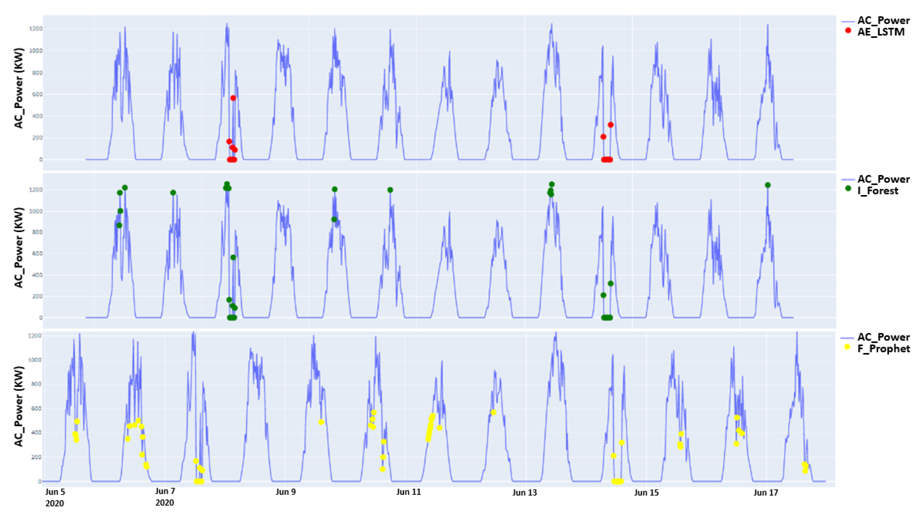
  • The investigation of three well-known anomaly detection models: Autoencoder LSTM (AE-LSTM), Facebook-Prophet, and Isolation Forest. Comparison tests were conducted examining the accuracy and performance of these models with their optimized hyperparameters.
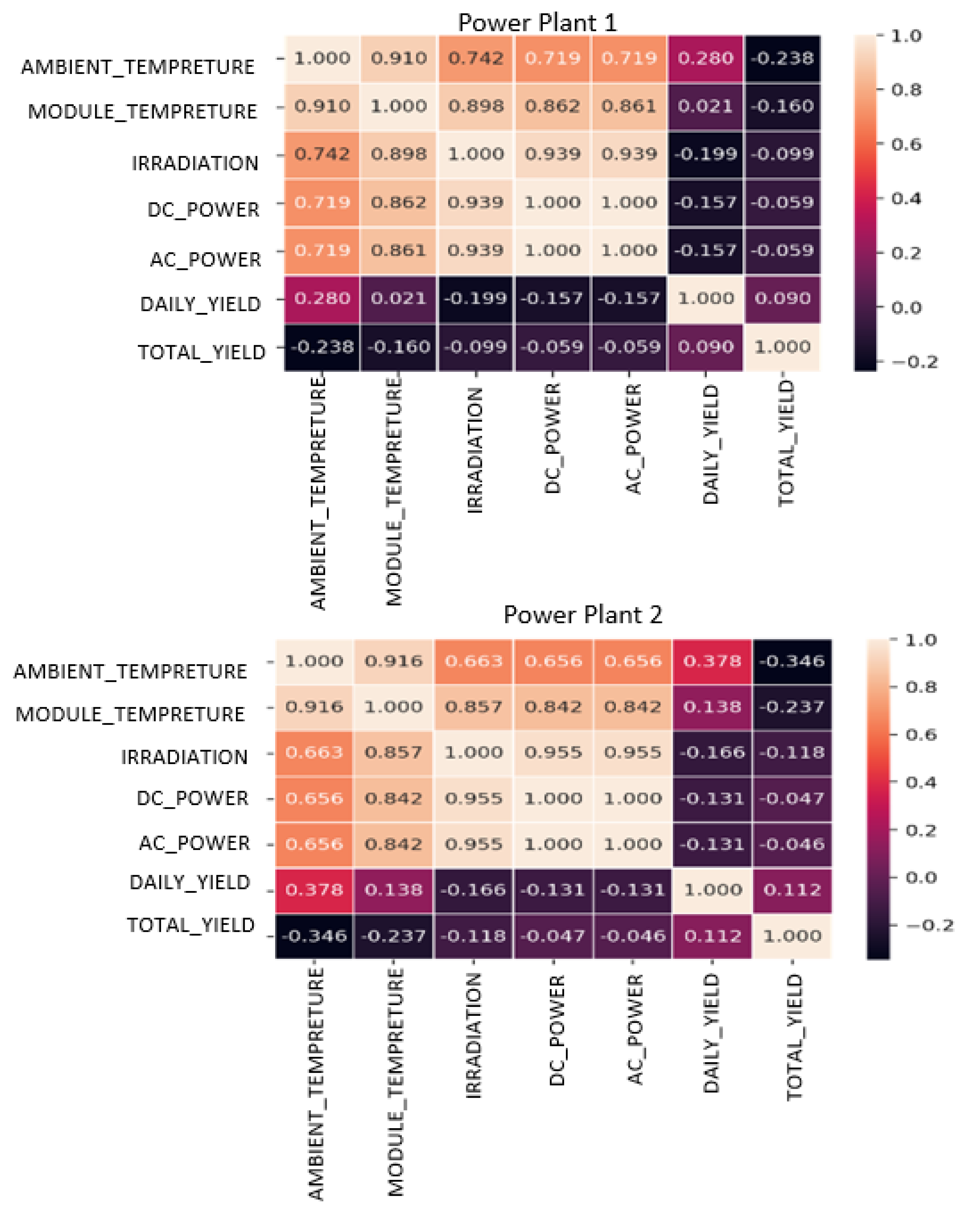
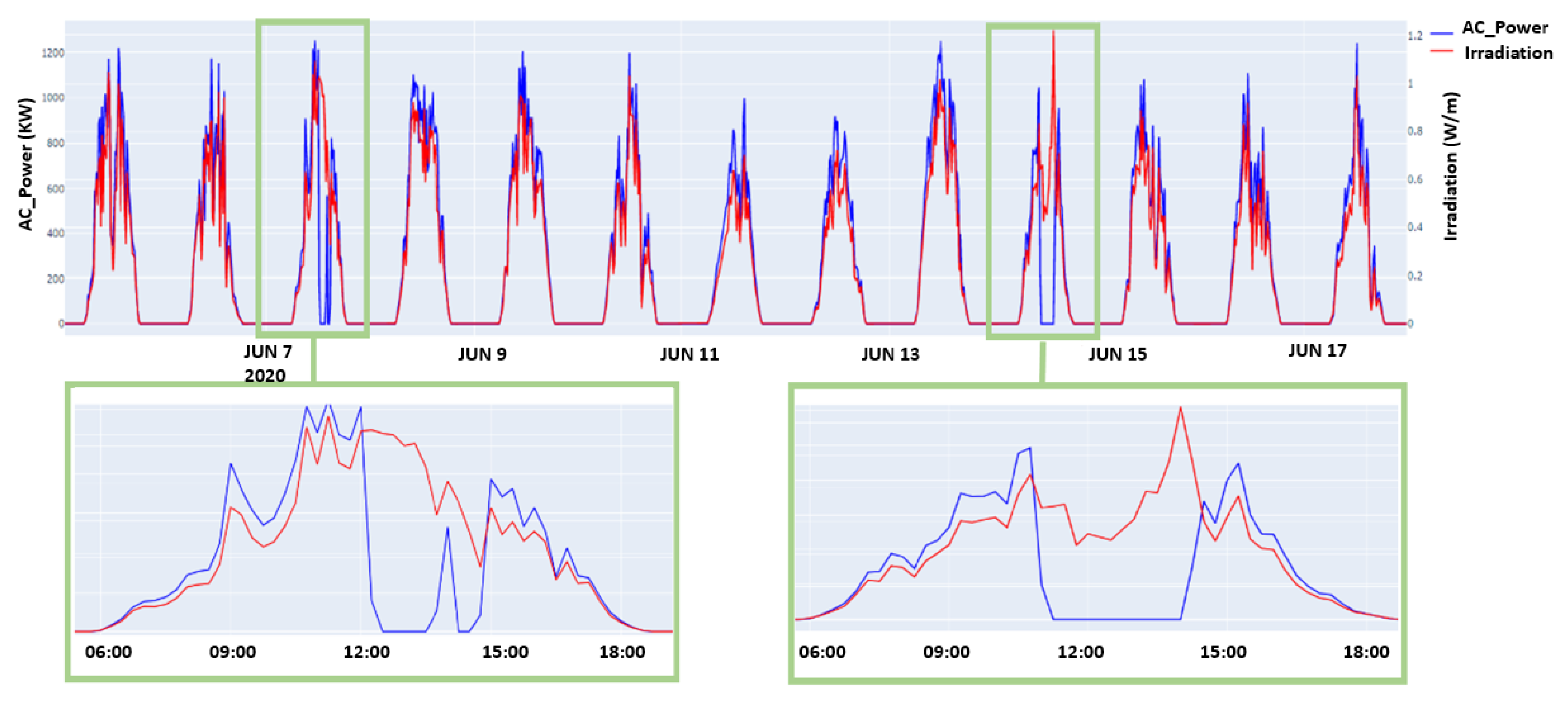
  • Defining and classifying the internal and external factors that induce anomalies in the PV power plant, investigating their effects on the model’s accuracy, and studying the correlation effect and its impact on detecting anomalies.
In the remainder of this paper, Section 2 discuss the paper background and relevant work. Section 3 characterizes the used machine learning algorithms. Section 4 characterizes the collected datasets. Section 5 demonstrates the experimental outputs and parameters optimization. In the end, we gather our outcomes and presents some future directions at Section 6.

2. Related Work

Several works have investigated anomaly detection techniques in photovoltaic (PV) power systems. For instance, reference [6] compared multiple methods to disclose and categorize abnormalities containing the auto-regressive integrated moving average model (ARIMA), neural networks, support vector machines, and k-nearest-neighbors classification. In [15], the authors implemented an abnormality exposure and predictive maintenance scheme for PV layout. The model is implemented to anticipate the AC power generation built on an ANN, which determines the AC power generation utilizing solar irradiance and temperature of PV panel data. A new technique for fault detection is proposed by [16] built on thermal image processing with an SVM tool that classifies the attributes as defective and non-defective types.
A model-based anomaly detection technique is proposed by [17] for inspecting the DC part of PV plants and momentary shading. Initially, a model based on the one-diode model is composed to outline the ordinary nature of the supervised PV system and form residuals for fault detection. Next, a one-class support vector machine (1-SVM) process is implemented to residuals starting with the running model for fault disclosure. Reference [18] presented SunDown, a sensorless method for disclosing per-panel faults in solar arrays. SunDown’s model-driven method influences interactions among the power generated by adjoining panels to detect disparities from anticipated nature. The model can manage simultaneous faults in many panels and classify anomalies to decide possible sources including snow, leaves, debris, and electrical failures.
A new tool (called ISDIPV) is presented by [19], which is capable of detecting anomalies and diagnosing them in a PV solar power plant. It includes three fundamental operational items for data acquisition, anomaly detection, and diagnosis of the disclosed disparities regarding regular performance. Two forms of modeling methods were implemented to describe the ordinary performance anticipated: linear transfer functions (LTF) and neural networks models built on multilayer perceptrons (MLP). The research in [20] presented a data-driven answer for adequate anomaly detection and classification, which applied PV string currents as signs to disclose and classify PV systems anomalies. The proposed anomaly detection approach used unsupervised machine learning techniques. The approach included two phases, particularly local context-aware detection (LCAD) and global context-aware anomaly detection (GCAD).
Anomalies related to TeleInfra base stations’ fuel consumption were detected by [21] in the registered data utilizing the generator as an origin of power. Anomalies were detected through learning the patterns of the fuel consumption applying four classification methods: support vector machines (SVM), k-nearest neighbors (KNN), logistic regression (LR), and multilayer perceptron (MLP). The results showed that MLP is the most efficient in the interpretation measurement.
A new technique is presented by [4] for monitoring PV systems by detecting anomalies using “k-nearest neighbors (kNN)” and “one-class support vector machine (OCSVM)”. The self-learning algorithms markedly decreased the measuring exertion and supported the reliable monitoring of faults. The authors of [22] used a k-nearest-neighbors algorithm and a multilayer perceptron to process the data from a DC sensor and detect differing attributes of the electrical current. A sensorless detection approach is proposed by [5] that is controlled by the rapid current decline enclosed by two maximum power point tracking (MPPT) sampling moments in PV plants. Simulations were executed to validate its possibility to determine anomalies against fluctuating environments, regardless of the discrepancy and irradiance ranks.
An anomaly detection framework of monocrystalline solar cells is proposed by [23]. The framework has two stages: In the initial stage, a generative adversarial network (GAN) is applied to construct an anomaly detection model. This model permits the detection of abnormal compositions using only non-defective samples for training. Next, the discovered anomalies will be employed as generated features for the supervised training of a fully convolutional network.
An analytical scheme is presented by [24] for online investigation of the raw video streams of aerial thermography. This scheme combines image processing and statistical machine learning methods. The presented scheme depends on robust principal component analysis (RPCA), which is utilized on PV images for the concurrent detection and confinement of anomalies. In addition to RPCA, post-processing procedures are proposed for image noise reduction and segmentation. Distinct models are chosen by [25] for the energy yield data examination. These are linear models, proximity-based models, probabilistic models, anomaly ensembles, and neural networks that have the highest detection rate.
SolarClique, a data-driven method, is considered by [26] to detect anomalies in the power generation of a solar establishment. The method does not need any sensor apparatus for fault/anomaly detection. Instead, it exclusively needs the assembly outcome of the array and those of close arrays for operating anomaly detection. An anomaly detection technique utilizing a semi-supervision learning model is suggested by [27] to predetermine solar panel conditions for bypassing the circumstance that the solar panel cannot produce power precisely as a result of equipment deterioration. This method utilizes the clustering model for regular actions filtration and the neuron network model, Autoencoder, to establish the classification.
A general, unsupervised, and scalable scheme is presented by [28] to detect anomalies in time-series data that can run offline and online. The scheme is composed of a rebuilding model following a variational autoencoder. Both the encoder and decoder are parametrized with recurrent neural networks to recognize the temporal reliance of time-series data. The outcomes illustrate that the model can detect anomalous arrangements by utilizing probabilistic restoration metrics such as anomaly scores. Reference [29] proposed a new ensemble model anomaly detection approach with non-linear regression models and anomaly scores following correlation study adapted for cyber-physical intrusion detection in smart grids.
The unsupervised contextual and collective detection approach is utilized by [30] to data flow by a huge energy dispenser in the Czech Republic. The approach examines distinctive forms of potential abnormalities (e.g., above/below-voltages). Common item-set mining and categorical clustering techniques are used along with clustering silhouette thresholding to identify anomalies. A recent survey is presented by [31] of distinct anomaly detection methods. These techniques consist of classification, nearest neighbor, clustering, statistical, spectral, information–theoretic, and graph. Selecting the convenient AD algorithm relies on input data, the form of anomalies, output data, and domain knowledge.

3. Materials and Methods: ML Algorithms

Different techniques and methods used in this paper are discussed in this section. Namely, we shed more light on the used ML algorithms (i) AutoEncoder Long Short-Term Memory (AE-LSTM), (ii) Facebook-Prophet, and (iii) Isolation Forest. These algorithm architectures are intensively discussed, creating a solid understanding of this research methodology.

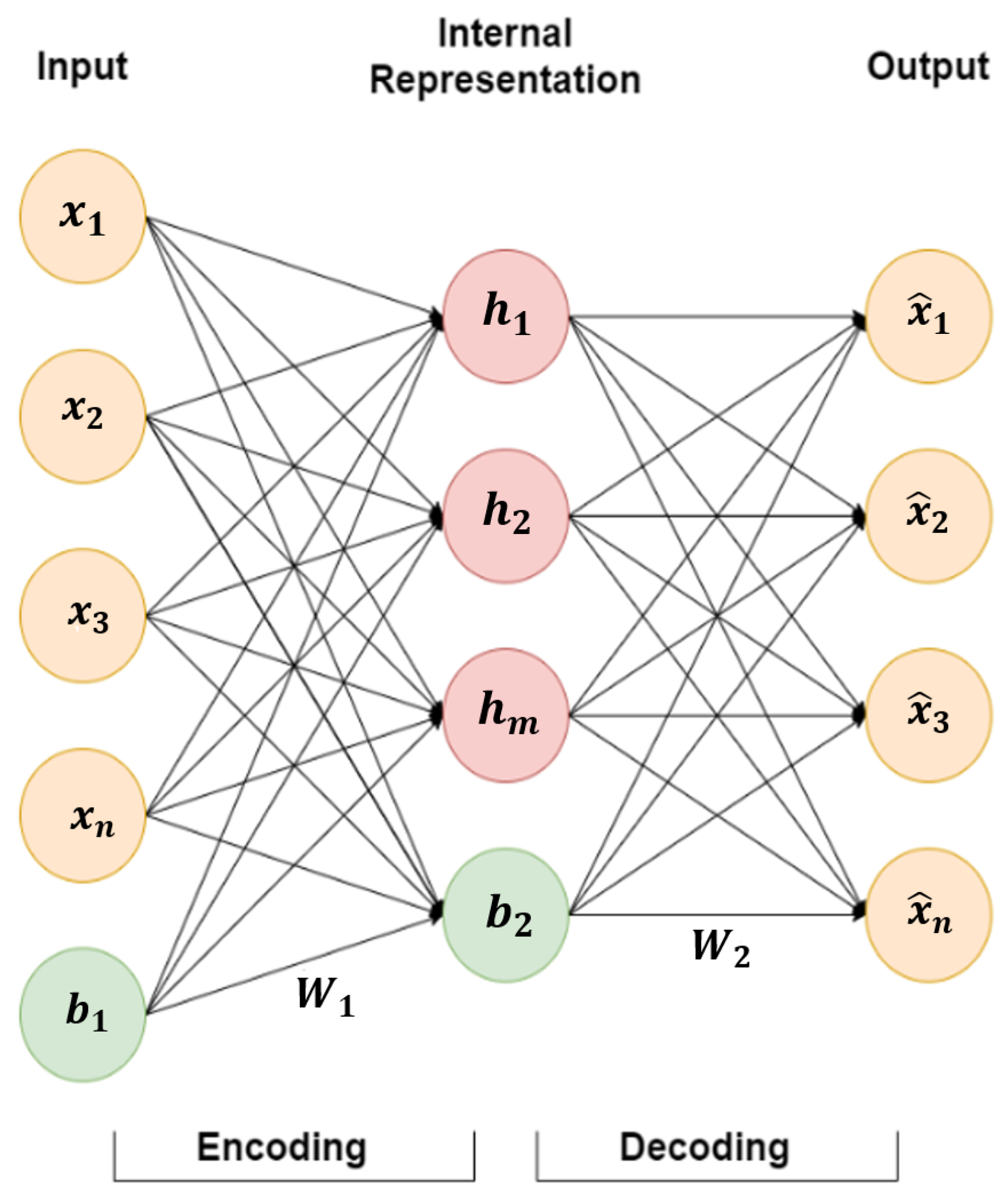
3.1. AutoEncoder Long Short-Term Memory (AE-LSTM)

AutoEncoder (AE) is an unsupervised ANN. It has the same structure of three symmetrical layers: input, hidden (interval description), and an output layer (remodeling) [32]. It has internal encoding and decoding processes. The encoding starts from the input to the hidden layer, whereas decoding handles the hidden layer to the output layer. AE has the merit of learning unlabelled data efficiently to predict from the input vector. Figure 1 illustrates the construction of AE.
The encoding process is described by:
H = f 1 W i · X + b i
where W i and b i are the weights and bias parameters among the input and the hidden layer. X is the primary input, H is the intermediate representation of the primary data, and f 1 is the activation function (e.g., ReLU, Logistic (Sigmoid) and TanH). Likewise, the decoding process is expressed as:
X ^ = f 2 W h · H + b h
where W h and b h are the weights and bias parameters between the hidden and the output layer, respectively. X ^ is the output that is reconstructed from the input data. AE is trained with the objective of minimizing the difference between the output X ^ and the input vector X through squared error [33], also called the reconstruction error [32], which is represented by:
L ( X , X ^ ) = X ^ X 2 .
Long Short-Term Memory (LSTM) is part of recurrent neural networks (RNNs). It employs an enclosed state (memory) to handle time-series inputs to hold the sequence relation of the input vector X [34]. It also uses the backpropagation through time (BPTT) model [35], but this causes a gradient vanishing. Therefore, LSTM uses three controlling gates: the input, forget, and output gates and the memory cell that memorizes a temporal state. The gates can reduce the gradient vanishing intensively by renewing and controlling the data flow [34]. Figure 2 illustrates the LSTM unit.
LSTM controls the information flow through the gates using the following equations:
i t = σ W i x t , h t 1 + b i
f t = σ W f x t , h t 1 + b f
u t = tanh W u x t , h t 1 + b u
o t = σ W o x t , h t 1 + b o
c t = f t c t 1 + i t u t
h t = o t tanh c t
where h t is the present final output, c t is the current cell state, x t is the present input, f t is the forget gate, i t is the input gate, u t is the input to the cell c that is gated by the input gate, o t is the output control signal, and ⊙ is an element-wise multiplication [34]. The AE-LSTM neural network learns the correlation among input variables and the correlation in the time series. The LSTM entity also avoids the issue of long-term memory reliance.

3.2. Facebook-Prophet

A prophet is a time-series forecasting algorithm; it extends Twitter’s Anomaly Detection (TAD) by replacing the residual component with holidays to detect changepoints [36]. Prophet separates a time series into three elements, seasonal, trend, and holidays, as follows:
y ( t ) = g ( t ) + s ( t ) + h ( t ) + ϵ t
where g ( t ) is the trend function that captures non-seasonal changes, s ( t ) is the seasonal changes function, and h ( t ) is the holiday’s function. ϵ t is a function that seizes any other changes that do not fit the three main functions. g ( t ) has both saturating growth and piecewise linear models [36]. g ( t ) defines the logistic growth model as follows:
g ( t ) = c 1 + exp ( ( k ( t ( m ) ) ) )
where c is the carrying capacity, k is the growth rate, and m is an offset specification. g ( t ) then incorporates trend updates in the growth model by describing change points s j where the growth rate is permitted to update at time t. Assume there exist S changepoints at times s j , where j = 1 , , S . Designate a vector of rate adjustments δ R S , where δ j is the change in rate that happens at time s j . The rate at time t is defined as follows:
t = k + a ( t ) T δ
where a ( t ) T δ is the cumulative growth until changepoints s j [37] and a ( t ) { 0 , 1 } S is a vector that can be computed as follows [36]:
a j ( t ) = 1 , if t s j 0 , Otherwise .
Then, the prophet modifies the primary logistic growth model to include trend updates for non-linear, saturating growth as follows:
g ( t ) = c ( t ) 1 + exp ( ( k + a ( t ) T δ ) ( t ( m + a ( t ) T γ ) ) )
and the linear growth can be draft as follows:
g ( t ) = k + a ( t ) T δ t + m + a ( t ) T γ .
Let δ R S such that points in δ are the rate of modifications in g ( t ) . The allocation of change points is made by assigning δ using Laplacian distribution δ j Laplace ( 0 , τ ) , where τ controls the compliance of growth rate [37] and γ j is set to s j δ j to make the function continuous [36].

3.3. Isolation Forest

Isolation Forest is an unsupervised anomaly detection model built on decision trees. It defines anomalies as data points that are limited and abnormal [38]. Isolation Forest works by defining a tree structure based on randomly selected features and then processing a sample of the data picked randomly into the tree [38]. The branching structure process is done with a random threshold selected in the range of the selected feature’s minimum and maximum values. If a sample goes deeper into the tree, it is unlikely to be an anomaly. On the contrary, if the sample is positioned in shorter branches, it is more likely to be an anomaly [38].
The algorithm can be described as follows: Let T be a node in the tree, q is a sample of selected features, p is the threshold value, and X = x 1 , x 2 , x 3 , x 4 , , x n is the dataset with n samples where each sample has d features. T can be a leaf node or can be an inside node (with two sub-nodes T l e f t , T r i g h t ). If the threshold p > q , then the sample will be maintained to the T l e f t . Otherwise, the sample will be assigned to T r i g h t . This process keeps repeating until either all data at the node have similar values, or the node has one sample only, or the tree reaches the maximum possible depth (length). The length of path h ( x ) can be determined by counting the edges that connect the tree from the root node to an outside node. The smaller h ( x ) means that sample x is more likely to be defined as an anomaly. The anomaly score s of the sample x can be computed as:
s ( x , n ) = 2 E ( h ( x ) ) c ( n )
where c ( n ) is the evaluation of average h ( x ) for the outside node and can be computed as:
c ( n ) = 2 H ( n 1 ) 2 ( n 1 ) n for n > 2 1 for n = 2 0 otherwise
where H ( i ) expresses the harmonic that can be evaluated by ln ( i ) + γ , (γ represents Euler’s constant) [38].

4. Collected Data

The used data were collected at two solar power plants in India (plant 1 is near Gandikotta, Andhra, and plant 2 is near Nasik, Maharashtra) over 34 days, each with 15 min intervals. Every plant included 22 inverter sensors connected at both the inverter and the plant levels to measure the generation rate (an internal factor that could cause anomalies), such as AC and DC powers. At the plant level, the inverter measured the irradiation, the ambient, and the module temperatures (they represented the external factors that could cause anomalies) for weather measurements. The data were published, licensed, and accessed under [39].
Figure 3 shows the correlation matrix denoting the correlation coefficients among the characteristic elements. The matrix computes a linear correlation among variables, where −1 means that the correlated variables have a powerful negative correlation, and 1 indicates a strong positive correlation. The diagonal values give the dependence of a variable by its own (also called autocorrelation). Spearman’s rank correlation [40] is used to determine the correlation rank between features as follows:
ρ = 1 6 d i 2 n n 2 1
where ρ is the Spearman’s rank correlation coefficient, d i is the difference among the two ranks for every observation, and n is the number of observations. The figure shows that both internal and external factors are highly correlated except for the daily and the total yields. The daily yield represents all the generated power in KW for this particular inverter until the recorded time t. On the other hand, the total yield is the summation of all the generated power from the 22 inverters in this specific plant. In the future, we will also consider allocating data in federated architectures [41].

5. Results and Discussion

This section explains the experimental evaluation carried out to validate and evaluate the paper claims. A complete description of the experimental setup is provided. Following, we analyze our findings and results in detail.
PV systems may have many types of anomalies. To make a proper comparison between the used anomaly detection algorithms, tests were conducted to investigate the effect of both internal and external factors as well the correlation effect on the data of all inverter sensors for the two plants. For instance, a test was done to compare the generated AC power and the irradiation for inverter number 1 of power plant 1, as illustrated in Figure 4. It can be noticed that there was a drop in the AC power in the periods of 7 June and 14 June. This notice can indicate a failure at the inverter level.
The number of anomalies in the signal is 13, which were distributed on 7 June and 14 June. On the contrary, for other inverters such as inverter number 12, there was no drop in the AC power generation, as illustrated in Figure 5.
Before testing the candidate algorithms, the grid parameters search optimizer, supported by Scikit learn [42], was used to tune each algorithm’s hyperparameters. The optimizer explores all possible combinations of a defined range of values for each parameter until the best accuracy is obtained. This measure means that an appropriate objective function can be defined for each algorithm to select the optimal parameters. The algorithms are tested on the AC Power signal from inverter number 1 in power plant 1 to detect the 13 true anomalies. The algorithm’s parameters and optimizer results are stated in the following subsections.

5.1. Facebook-Prophet Optimized Parameters

An essential parameter in Facebook-Prophet is the number of change points (n-changepoints) in the dataset. Its usual value is 25. Change points are uniformly distributed on the first 80% of the time-series signal. The changepoint_prior_scale indicates how flexible the change points are allowed to be, which means how much the change points can suit the data. Its usual value is 0.05. The seasonality_mode parameter defines two modes: the additive and multiplicative modes. The default mode is additive, which signifies that the seasonality’s impact is combined with the forecast trend. Table 1 shows the parameters grid for Prophet with a total of 162 possible models.
Due to the working principle of Prophet of predicting a time-series signal, the objective functions were selected to be R-squared ( R 2 ), Mean Squared Error (MSE), and Mean Absolute Error (MAE). They can be computed as follows:
R 2 = i = 1 N i y i Y ^ i i = 1 N i y i Y ¯ i
M S E = i = 1 N i y i Y ^ i 2 N i
MAE = 1 N i = 1 N y i Y ^ i
where y, Y ^ are the actual and the predicted data, respectively, whereas Y ¯ is the mean value of actual data. The optimization results found the best R 2 = 87.448%, MAE = 76.125 KW, and MSE = 135.013 KW for the following optimal parameters:
  • n_changepoints = 0.9;
  • changepoint_prior_scale = 200;
  • seasonality_mode = multiplicative.
The R 2 shows a high value that describes an acceptable prediction accuracy, while the MAE and MSE show that the model has an acceptable error in forecasting the AC power signal whose values lie in the range of 1200–1400 KW.

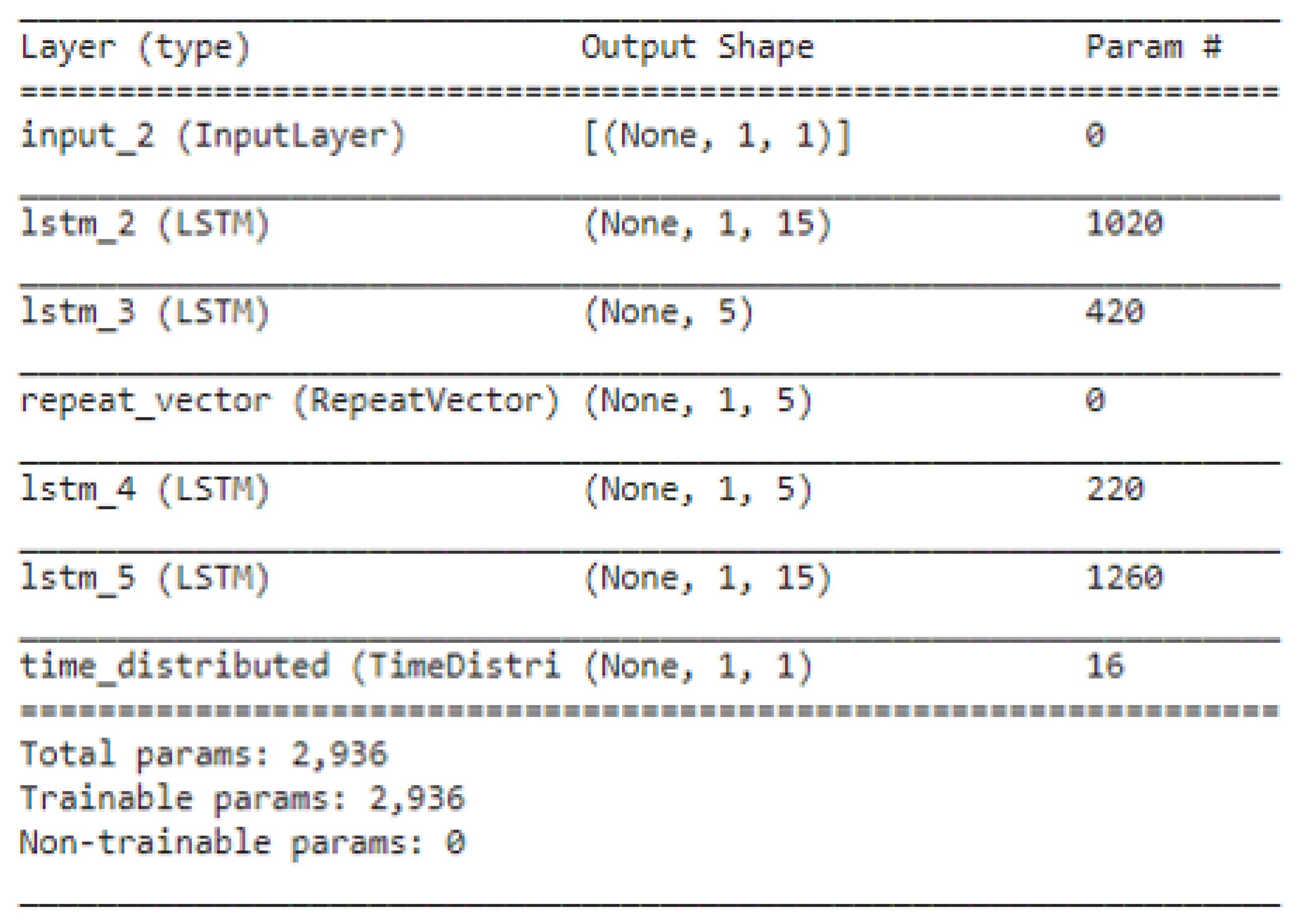
5.2. AE-LSTM Optimized Parameters

AE-LSTM, on the contrary, shares the same parameters that any other neural network model has, which are the number of hidden neurons, the number of layers, activation function, epochs, and batch size. For simplification, the number of hidden layers was chosen to be four layers with Rectifier (ReLU) activation function, and the number of hidden neurons was optimized for each layer separately. Table 2 shows the parameters grid for AE-LSTM with a total of 54,432 possible models:
The AE-LSTM also learns/trains on a time-series signal and then tries to predict/ forecast these signal characteristics in the future. Therefore, the same as in Prophet, the R 2 , MSE, and MAE were used as objective functions. The optimization results found the best R 2 = 98.1749%, MAE = 12.733 KW, and MSE = 20.934 KW for the optimal parameters epochs (200) and batch size of 20. The number of hidden neurons and the complete AE-LSTM model are illustrated in Figure 6.

5.3. Isolation Forest Optimized Parameters

Isolation Forest was also optimized for the number of estimators (n_estimators) or trees in the ensemble. In other words, it is the number of trees that will construct the forest. It has a default value of 100. Another parameter is the contamination, which describes the expected proportion or rate of outliers/abnormality in the dataset. Table 3 shows the parameters grid for AE-LSTM with a total of 338 possible models. The bootstrap is a parameter that controls the sampling process. If it is set to True, then the exclusive trees fit random subsets of the training data sampled with replacement. If it is set to False, then sampling without replacement is conducted.
The Isolation Forest does not predict any time-series signal compared to Prophet and AE-LSTM. Instead, it classifies the data points into normal and abnormal, with the same concept as random forest. Therefore, the objective function will focus on the number of true and false anomalies. The optimization results for 338 possible models found only one value, which is 25 anomalies, where 12 points are true anomalies, and the other 13 points are false anomalies. These results are represented in a confusion matrix, as shown in Table 4.
The confusion matrix can be used to compute the accuracy, precision, sensitivity, and F 1 Score. Their formulas are given as follows:
Accuracy = T P + T N T P + F P + F N + T N
Precision = T P T P + F P
Sensitivity = T P T P + F N
F 1 Score = 2 ( Recall + Precision ) ( Recall + Precision ) .
The computed values are as follows: accuracy = 0.8963, precision = 0.9474, sensitivity = 0.9432, and F1 Score = 0.9453.

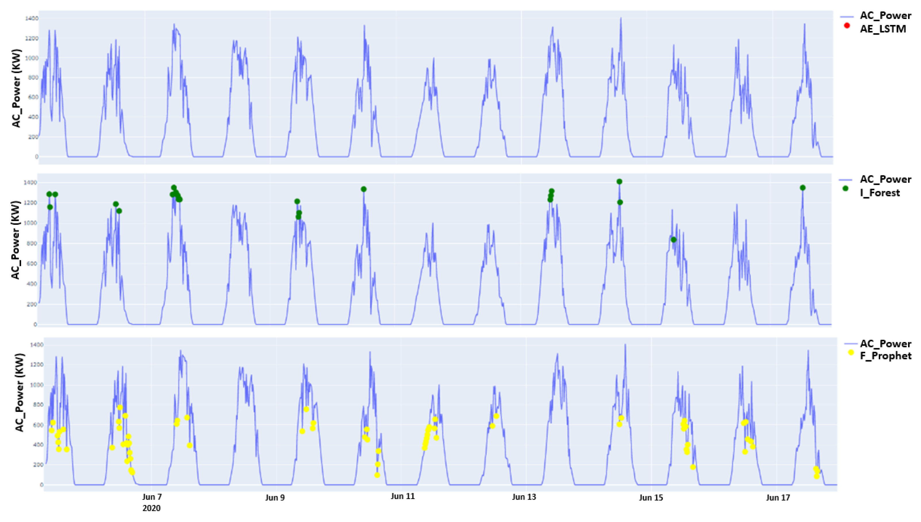
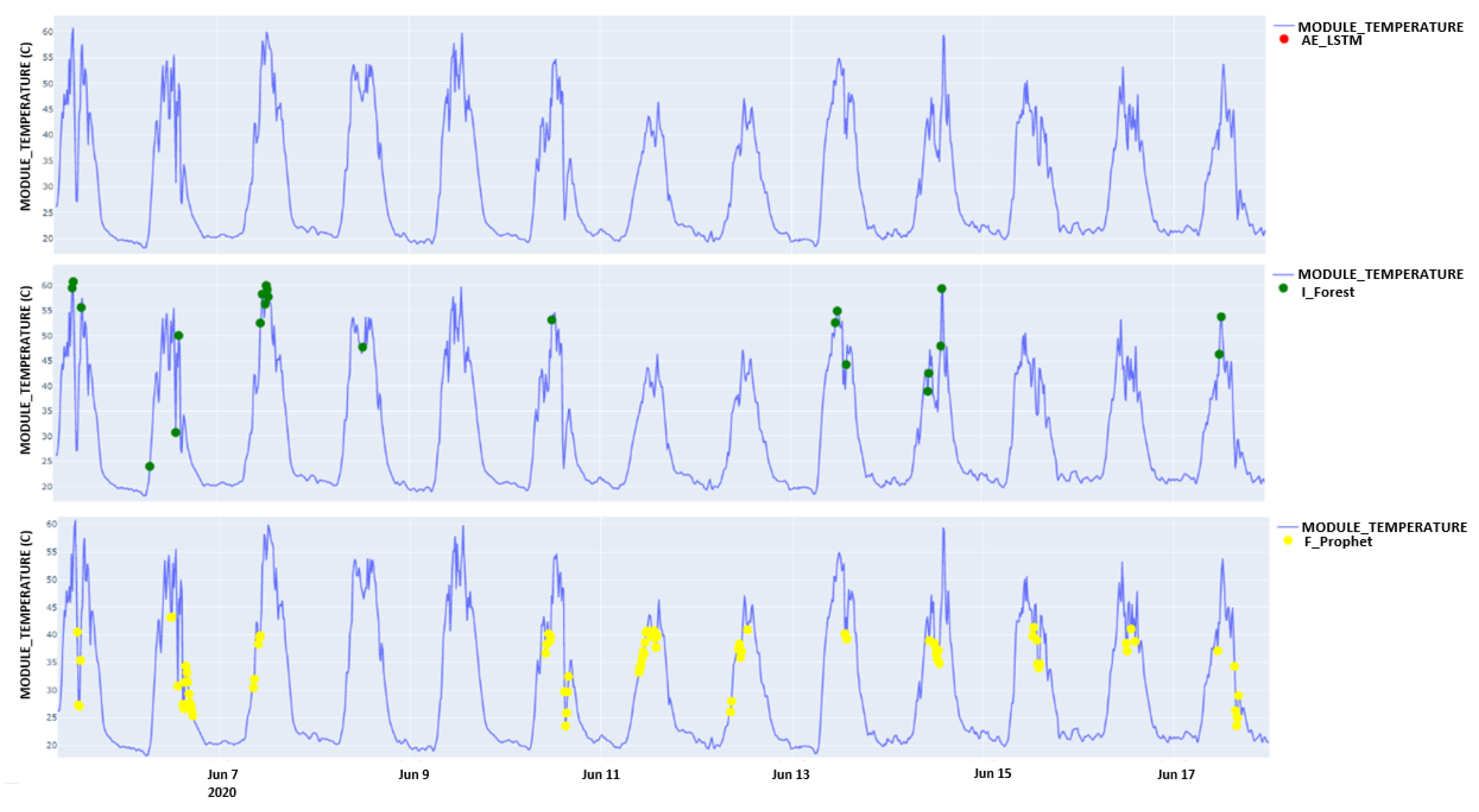
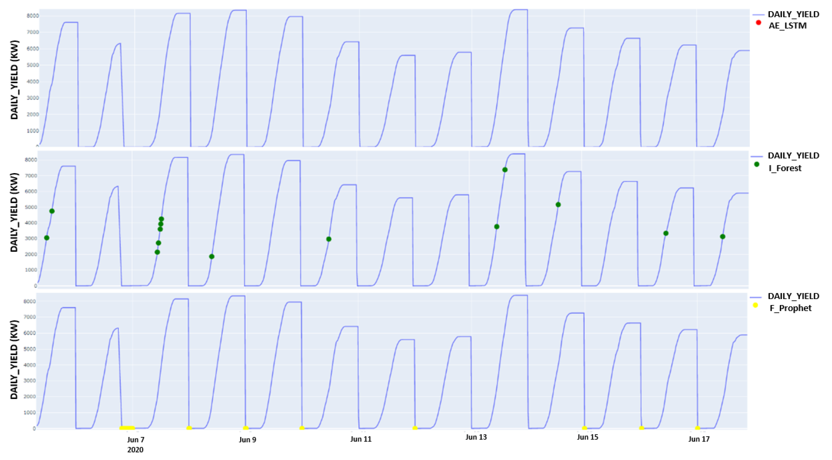
5.4. Anomaly Detection Performance

The Isolation Forest, AE-LSTM, and Prophet algorithms are implemented to evaluate their performance in detecting the AC-generated power signal abnormalities. The outcomes are illustrated in Figure 7. It can be noticed that even though Prophet detected the anomalies on 7 and 14 June, it failed to determine the healthy signal by labeling it as an anomaly with a total of 53 anomalies (false anomalies). Isolation Forest also detected the true positive anomalies but marked all the signal peaks as anomalies with 25 outliers. The AE-LSTM detected the correct 13 anomalies compared to the irradiation signal, thus indicating a fault in the inverter module. It was also successful in identifying the healthy signal. Hence, the inverter module is working well. In addition, the models are tested on a healthy AC Power signal from inverter number 12. Prophet and Isolation Forest found anomalies within this signal. It is worth mentioning that the Isolation Forest detected false anomalies on the peaks, while AE-LSTM determined that there are no anomalies, as shown in Figure 8.
The second test investigated the external correlated factor of module temperature, as shown in Figure 9. It can be seen that the signal is healthy. However, the Prophet found anomalies within a complete healthy signal. The Isolation Forest detected false anomalies on the peaks, and the AE-LSTM determined that it is a healthy signal and thus detected no anomalies. This experiment indicates that the temperature module does not need to be maintained for the next tested time interval, and it is working correctly.
The third test examined the effect of the uncorrelated internal factors, which are expressed in the daily yield. The daily yield signal is a healthy signal with no apparent anomalies that could be determined. This signal means that even if there is a failure in one of the 22 inverters, it did not affect the daily yield signal. The Prophet and Isolation Forest also failed this test, while AE-LSTM succeeded in determining no anomalies in a healthy signal, as shown in Figure 10.
The results above showed that the AE-LSTM was the most accurate in detecting the true anomalies without tagging false positive points (normal) as anomalies. In addition, we proved that the two optimized models did not accurately distinguish the correct and the false anomalies. On the contrary, although Prophet and Isolation Forest found the true anomalies, both models labeled healthy/normal points as anomalies. Furthermore, the results demonstrated that Prophet and Isolation Forest are more sensitive to noisy signals and need more datasets to generalize and capture signal characteristics to distinguish a false from a true anomaly. Interesting future work would be investigating the blockchain technology for the large-scale solar power plant networks [43] and examining recent trends in machine learning such as active machine learning [44]. These findings may assist in maintaining the plant at the component level by scheduling a time to repair the faulted inverters all at once, thus reducing the off-time during which other components can still operate properly.
It is worth mentioning that the genetic algorithm (GA) serves as an alternative to the grid search method used in this work. GA is a metaheuristic search method originating from the theory of evolution. It can be used to select values under given constraints that achieve a lower loss of a defined objective function [45]. GA was not implemented in our work because the range of changes in the algorithm’s accuracy was relatively small; therefore, the grid search method was used instead. Future work may include the application of GA for intelligent anomaly mitigation techniques.

6. Conclusions

Anomaly detection in modern solar power plants using data-driven approaches is vital in reducing downtimes and increasing efficiency. In this paper, three machine learning models’ performances were analyzed to illustrate the most exemplary model that can precisely determine the abnormalities in the photovoltaic (PV) system. The correlation coefficients between the plants’ internal and external feature parameters were determined and used to analyze the efficiency of machine learning models in detecting anomalies. The AE-LSTM detected anomalies and successfully identified the healthy signal. Future work would include the investigation of intelligent anomaly mitigation techniques. In addition, an interesting area to investigate would be employing the recent distributed machine learning trend, i.e., federated learning, in large-scale intelligent solar power grids.

Author Contributions

Conceptualization, M.I. and F.M.A.; Methodology, M.I.; Software, M.I. and A.A.; Validation, M.I. and A.A.; Formal Analysis M.I. and F.M.A.; Investigation, M.I. and A.A.; Resources, M.I. and F.M.A.; Data Curation, M.I. and A.A.; Writing—Original Draft Preparation, M.I. and A.A.; Writing—Review & Editing, M.I., A.A., F.M.A. and M.D.A.; Visualization, M.I. and A.A.; Supervision, M.I.; Project Administration, M.I. and F.M.A.; Funding Acquisition, M.I. and F.M.A. All authors have read and agreed to the published version of the manuscript.

Funding

This research was funded by Deanship of Graduate Studies and Scientific Research at the German Jordanian University, Seed fund SATS 03/2020.

Institutional Review Board Statement

Not applicable.

Informed Consent Statement

Not applicable.

Data Availability Statement

Publicly available datasets were analyzed in this study. This data can be found here: https://www.kaggle.com/anikannal/solar-power-generation-data (accessed on 25 January 2022).

Acknowledgments

This research has been financed by the Europan Social Fund. The authors would like to acknowledge the Deanship of Graduate Studies and Scientific Research at the German Jordanian University for the Seed fund SATS 03/2020. Feras M. Awaysheh acknowledges support via IT Academy program and the European Regional Development Funds via the Mobilitas Plus programme (grant MOBTT75). In addition, Taif University Research supporting, project number (TURSP-2020/126), Taif university, Taif Saudi Arabia.

Conflicts of Interest

The authors declare no conflict of interest.

Abbreviations

The used acronyms and notations in the paper.
Acronyms
PVPhotovoltaic
AE-LSTMAutoEncoder Long Short-Term Memory
ANNArtificial neural network
RNNRecurrent neural networks
R 2 R-squared
ReLURectifier activation function
1-SVMOne-class support vector machine
F P r o p h e t Facebook-Prophet
I F o r e s t Isolation Forest
Notations
XInput vector of AutoEncoder
X ^ Predicted output vector of AutoEncoder
W i Weights
b i Bias
f 1 Activation function
HIntermediate representation of the primary data
h t The present final output
c t Current cell state
x t Present input
f t Forget gate
i t Input gate
u t The input to the cell c that is gated by the input gate
o t The output control signal
An element-wise multiplication
g ( t ) Trend function
h ( t ) The holidays function
CThe carrying capacity
kThe growth rate
mAn offset specification
s i Change points
δ Vector of rate adjustments
a ( t ) T δ         The cumulative growth until change points s j
pThe threshold value
qA sample of selected features
h ( x ) The length of path
H ( i ) The harmonic
ρ Spearman’s rank
d i The difference among the two ranks of each observation
yThe actual data
Y ^ The predicted data

References

  1. Awaysheh, F.M.; Alazab, M.; Garg, S.; Niyato, D.; Verikoukis, C. Big data resource management & networks: Taxonomy, survey, and future directions. IEEE Commun. Surv. Tutor. 2021, 23, 2098–2130. [Google Scholar]
  2. Alshehri, M.; Kumar, M.; Bhardwaj, A.; Mishra, S.; Gyani, J. Deep Learning Based Approach to Classify Saline Particles in Sea Water. Water 2021, 13, 1251. [Google Scholar] [CrossRef]
  3. Agarwal, A.; Sharma, P.; Alshehri, M.; Mohamed, A.A.; Alfarraj, O. Classification model for accuracy and intrusion detection using machine learning approach. PeerJ Comput. Sci. 2021, 7, e437. [Google Scholar] [CrossRef]
  4. Benninger, M.; Hofmann, M.; Liebschner, M. Online Monitoring System for Photovoltaic Systems Using Anomaly Detection with Machine Learning. In Proceedings of the NEIS 2019, Conference on Sustainable Energy Supply and Energy Storage Systems, Hamburg, Germany, 19–20 September 2019; VDE: Hongkong, China, 2019; pp. 1–6. [Google Scholar]
  5. Li, C.; Yang, Y.; Zhang, K.; Zhu, C.; Wei, H. A fast MPPT-based anomaly detection and accurate fault diagnosis technique for PV arrays. Energy Convers. Manag. 2021, 234, 113950. [Google Scholar] [CrossRef]
  6. Hu, B. Solar Panel Anomaly Detection and Classification. Master’s Thesis, University of Waterloo, Waterloo, ON, Canada, 2012. [Google Scholar]
  7. Branco, P.; Gonçalves, F.; Costa, A.C. Tailored algorithms for anomaly detection in photovoltaic systems. Energies 2020, 13, 225. [Google Scholar] [CrossRef] [Green Version]
  8. Firth, S.K.; Lomas, K.J.; Rees, S.J. A simple model of PV system performance and its use in fault detection. Sol. Energy 2010, 84, 624–635. [Google Scholar] [CrossRef] [Green Version]
  9. Elsheikh, A.H.; Sharshir, S.W.; Abd Elaziz, M.; Kabeel, A.E.; Guilan, W.; Haiou, Z. Modeling of solar energy systems using artificial neural network: A comprehensive review. Sol. Energy 2019, 180, 622–639. [Google Scholar] [CrossRef]
  10. Elsheikh, A.H.; Katekar, V.P.; Muskens, O.L.; Deshmukh, S.S.; Abd Elaziz, M.; Dabour, S.M. Utilization of LSTM neural network for water production forecasting of a stepped solar still with a corrugated absorber plate. Process Saf. Environ. Prot. 2021, 148, 273–282. [Google Scholar] [CrossRef]
  11. Elsheikh, A.H.; Panchal, H.; Ahmadein, M.; Mosleh, A.O.; Sadasivuni, K.K.; Alsaleh, N.A. Productivity forecasting of solar distiller integrated with evacuated tubes and external condenser using artificial intelligence model and moth-flame optimizer. Case Stud. Therm. Eng. 2021, 28, 101671. [Google Scholar] [CrossRef]
  12. Ibrahim, M.; Alsheikh, A.; Al-Hindawi, Q.; Al-Dahidi, S.; ElMoaqet, H. Short-time wind speed forecast using artificial learning-based algorithms. Comput. Intell. Neurosci. 2020, 2020, 8439719. [Google Scholar] [CrossRef]
  13. Aslam, S.; Herodotou, H.; Mohsin, S.M.; Javaid, N.; Ashraf, N.; Aslam, S. A survey on deep learning methods for power load and renewable energy forecasting in smart microgrids. Renew. Sustain. Energy Rev. 2021, 144, 110992. [Google Scholar] [CrossRef]
  14. Latha, R.S.; Sreekanth, G.R.R.; Suganthe, R.C.; Selvaraj, R.E. A survey on the applications of Deep Neural Networks. In Proceedings of the 2021 IEEE International Conference on Computer Communication and Informatics (ICCCI), Coimbatore, India, 27–29 January 2021; pp. 1–3. [Google Scholar]
  15. De Benedetti, M.; Leonardi, F.; Messina, F.; Santoro, C.; Vasilakos, A. Anomaly detection and predictive maintenance for photovoltaic systems. Neurocomputing 2018, 310, 59–68. [Google Scholar] [CrossRef]
  16. Natarajan, K.; Bala, P.K.; Sampath, V. Fault Detection of Solar PV System Using SVM and Thermal Image Processing. Int. J. Renew. Energy Res. (IJRER) 2020, 10, 967–977. [Google Scholar]
  17. Harrou, F.; Dairi, A.; Taghezouit, B.; Sun, Y. An unsupervised monitoring procedure for detecting anomalies in photovoltaic systems using a one-class Support Vector Machine. Sol. Energy 2019, 179, 48–58. [Google Scholar] [CrossRef]
  18. Feng, M.; Bashir, N.; Shenoy, P.; Irwin, D.; Kosanovic, D. SunDown: Model-driven Per-Panel Solar Anomaly Detection for Residential Arrays. In Proceedings of the 3rd ACM SIGCAS Conference on Computing and Sustainable Societies, Guayaquil, Ecuador, 15–17 June 2020; pp. 291–295. [Google Scholar]
  19. Sanz-Bobi, M.A.; San Roque, A.M.; De Marcos, A.; Bada, M. Intelligent system for a remote diagnosis of a photovoltaic solar power plant. J. Phys. Conf. Ser. 2012, 364, 012119. [Google Scholar] [CrossRef] [Green Version]
  20. Zhao, Y.; Liu, Q.; Li, D.; Kang, D.; Lv, Q.; Shang, L. Hierarchical anomaly detection and multimodal classification in large-scale photovoltaic systems. IEEE Trans. Sustain. Energy 2018, 10, 1351–1361. [Google Scholar] [CrossRef]
  21. Mulongo, J.; Atemkeng, M.; Ansah-Narh, T.; Rockefeller, R.; Nguegnang, G.M.; Garuti, M.A. Anomaly detection in power generation plants using machine learning and neural networks. Appl. Artif. Intell. 2020, 34, 64–79. [Google Scholar] [CrossRef]
  22. Benninger, M.; Hofmann, M.; Liebschner, M. Anomaly detection by comparing photovoltaic systems with machine learning methods. In Proceedings of the NEIS 2020, Conference on Sustainable Energy Supply and Energy Storage Systems, Hamburg, Germany, 14–15 September 2020; VDE: Hongkong, China, 2020; pp. 1–6. [Google Scholar]
  23. Balzategui, J.; Eciolaza, L.; Maestro-Watson, D. Anomaly detection and automatic labeling for solar cell quality inspection based on Generative Adversarial Network. Sensors 2021, 21, 4361. [Google Scholar] [CrossRef]
  24. Wang, Q.; Paynabar, K.; Pacella, M. Online automatic anomaly detection for photovoltaic systems using thermography imaging and low rank matrix decomposition. J. Qual. Technol. 2021, 1–14. [Google Scholar] [CrossRef]
  25. Hempelmann, S.; Feng, L.; Basoglu, C.; Behrens, G.; Diehl, M.; Friedrich, W.; Brandt, S.; Pfeil, T. Evaluation of unsupervised anomaly detection approaches on photovoltaic monitoring data. In Proceedings of the 2020 47th IEEE Photovoltaic Specialists Conference (PVSC), Calgary, AB, Canada, 15 June–21 August 2020; pp. 2671–2674. [Google Scholar]
  26. Iyengar, S.; Lee, S.; Sheldon, D.; Shenoy, P. Solarclique: Detecting anomalies in residential solar arrays. In Proceedings of the 1st ACM SIGCAS Conference on Computing and Sustainable Societies, Menlo Park and San Jose, CA, USA, 20–22 June 2018; pp. 1–10. [Google Scholar]
  27. Tsai, C.W.; Yang, C.W.; Hsu, F.L.; Tang, H.M.; Fan, N.C.; Lin, C.Y. Anomaly Detection Mechanism for Solar Generation using Semi-supervision Learning Model. In Proceedings of the 2020 IEEE Indo–Taiwan 2nd International Conference on Computing, Analytics and Networks (Indo-Taiwan ICAN), Rajpura, India, 7–15 February 2020; pp. 9–13. [Google Scholar]
  28. Pereira, J.; Silveira, M. Unsupervised anomaly detection in energy time series data using variational recurrent autoencoders with attention. In Proceedings of the 2018 17th IEEE international conference on machine learning and applications (ICMLA), Orlando, FL, USA, 17–20 December 2018; pp. 1275–1282. [Google Scholar]
  29. Kosek, A.M.; Gehrke, O. Ensemble regression model-based anomaly detection for cyber-physical intrusion detection in smart grids. In Proceedings of the 2016 IEEE Electrical Power and Energy Conference (EPEC), Ottawa, ON, Canada, 12–14 October 2016; pp. 1–7. [Google Scholar]
  30. Rossi, B.; Chren, S.; Buhnova, B.; Pitner, T. Anomaly detection in smart grid data: An experience report. In Proceedings of the 2016 IEEE International Conference on Systems, Man, and Cybernetics (SMC), Budapest, Hungary, 9–12 October 2016; pp. 002313–002318. [Google Scholar]
  31. Toshniwal, A.; Mahesh, K.; Jayashree, R. Overview of anomaly detection techniques in machine learning. In Proceedings of the 2020 IEEE Fourth International Conference on I-SMAC (IoT in Social, Mobile, Analytics and Cloud) (I-SMAC), Palladam, India, 7–9 October 2020; pp. 808–815. [Google Scholar]
  32. Hu, D.; Zhang, C.; Yang, T.; Chen, G. Anomaly Detection of Power Plant Equipment Using Long Short-Term Memory Based Autoencoder Neural Network. Sensors 2020, 20, 6164. [Google Scholar] [CrossRef]
  33. Que, Z.; Liu, Y.; Guo, C.; Niu, X.; Zhu, Y.; Luk, W. Real-time Anomaly Detection for Flight Testing using AutoEncoder and LSTM. In Proceedings of the 2019 IEEE International Conference on Field-Programmable Technology (ICFPT), Tianjin, China, 9–13 December 2019; pp. 379–382. [Google Scholar]
  34. Hochreite, S.; Schmidhuber, J. Long short-term memory. Neural Comput. 1997, 9, 1735–1780. [Google Scholar] [CrossRef] [PubMed]
  35. Werbos, P.J. Backpropagation through time: What it does and how to do it. Proc. IEEE 1990, 78, 1550–1560. [Google Scholar] [CrossRef] [Green Version]
  36. Taylor, S.J.; Letham, B. Forecasting at scale. Am. Stat. 2018, 72, 37–45. [Google Scholar] [CrossRef]
  37. Srivastava, S. Benchmarking Facebook’s Prophet, PELT and Twitter’s Anomaly Detection and Automated de Ployment to Cloud. Master’s Thesis, University of Twente, Enschede, The Netherlands, 2019. [Google Scholar]
  38. Hariri, S.; Kind, M.C.; Brunner, R.J. Extended isolation forest. IEEE Trans. Knowl. Data Eng. 2019, 33, 1479–1489. [Google Scholar] [CrossRef] [Green Version]
  39. Kannal, A. Solar Power Generation Data. Kaggle.com. Available online: https://www.kaggle.com/anikannal/solar-power-generation-data (accessed on 25 January 2022).
  40. Corder, G.W.; Foreman, D.I. Nonparametric Statistics: A Step-by-Step Approach; John Wiley & Sons: Hoboken, NJ, USA, 2014. [Google Scholar]
  41. Awaysheh, F.M.; Alazab, M.; Gupta, M.; Pena, T.F.; Cabaleiro, J.C. Next-generation big data federation access control: A reference model. Future Gener. Comput. Syst. 2020, 108, 726–741. [Google Scholar] [CrossRef] [Green Version]
  42. ParameterGrid. Available online: https://scikit-learn.org/stable/modules/generated/sklearn.model_selection.ParameterGrid.html (accessed on 25 January 2022).
  43. Kebande, V.R.; Awaysheh, F.M.; Ikuesan, R.A.; Alawadi, S.A.; Alshehri, M.D. A Blockchain-Based Multi-Factor Authentication Model for a Cloud-Enabled Internet of Vehicles. Sensors 2021, 21, 6018. [Google Scholar] [CrossRef]
  44. Kebande, V.R.; Alawadi, S.; Awaysheh, F.M.; Persson, J.A. Active Machine Learning Adversarial Attack Detection in the User Feedback Process. IEEE Access 2021, 9, 36908–36923. [Google Scholar] [CrossRef]
  45. Whitley, D. A genetic algorithm tutorial. Stat. Comput. 1994, 4, 65–85. [Google Scholar] [CrossRef]
Figure 1. The AutoEncoder (AE) model.
Energies 15 01082 g001
Figure 2. Long Short-Term Memory (LSTM) unit.
Energies 15 01082 g002
Figure 3. Correlation matrix computing the linear correlation among the characteristic elements for power plants 1 and 2.
Energies 15 01082 g003
Figure 4. Signal comparison between AC, DC Power, Irradiation, and the Module Temperature signals from inverter number 12.
Energies 15 01082 g004
Figure 5. Signal comparison between AC, DC Power, Irradiation, and the Module Temperature signals from inverter number 12.
Energies 15 01082 g005
Figure 6. The AE-LSTM model.
Energies 15 01082 g006
Figure 7. Anomaly detection outcomes from the three models on a faulty AC Power signal.
Energies 15 01082 g007
Figure 8. Anomaly detection outcomes from the three models on a healthy AC Power signal.
Energies 15 01082 g008
Figure 9. Anomaly detection outcomes from the three models on a healthy module temperature signal.
Energies 15 01082 g009
Figure 10. Anomaly detection outcomes from the three models on a healthy daily yield signal.
Energies 15 01082 g010
Table 1. Grid parameters of Facebook-Prophet.
ParameterGrid
n_changepoints[10,25,50,75,100,150,200,300,400,500]
changepoint_prior_scale[0.1,0.2,0.3,0.4,0.5,0.6,0.7,0.8,0.9]
seasonality_mode[‘multiplicative’, ‘additive’]
Table 2. Grid parameters of AE-LSTM.
ParameterGrid
Number_hidden_neurons L1[5,10,15,20,25,30]
Number_hidden_neurons L2[5,10,15,20,25,30]
Number_hidden_neurons L3[5,10,15,20,25,30]
Number_hidden_neurons L4[5,10,15,20,25,30]
batch[5,10,15,20,25,30]
epochs[200,250,300,350,400,450,500]
Table 3. Grid parameters of Isolation Forest.
ParameterGrid
bootstrap[False, True]
n_estimators[50,100,200,300,400,500,600,700,800,900,1000,1500,2000]
contamination[0,0.01,0.03,0.06,0.09,0.12,0.15,0.2,0.25,0.3,0.4,0.45,0.5]
Table 4. The confusion matrix.
HealthyAnomaly
HealthyTrue Positives (TP) = 216False Negatives (FN) = 13
AnomalyFalse Positives (FP) = 0True Negatives (TN) = 12
Publisher’s Note: MDPI stays neutral with regard to jurisdictional claims in published maps and institutional affiliations.

