Impact of Dynamic Electricity Tariff and Home PV System Incentives on Electric Vehicle Charging Behavior: Study on Potential Grid Implications and Economic Effects for Households

Abstract

The rapid increase of electric vehicles (EVs) would lead to a rise in load demand on power grids but create different potential benefits as well. Those benefits comprise EVs serving as a mobile energy storage system to participate in adjusting the load on the power grids and helping manage renewable energy resources. This paper evaluates the effect of dynamic electricity prices and home photovoltaic (PV) system incentives on users’ EVs charging behavior and potential impacts on grid load and household economy. This has been done by establishing and assessing three different optimized charging configurations and comparing them to an uncontrolled charging strategy. In this study, the charging incentives are applied to a representative sample of 100 households with EVs and PV systems in a metropolitan area. The results show that an optimized charging strategy based on the dynamic electricity tariff can reduce charging costs by 18.5%, while a PV-based optimized strategy can reduce the costs by 33.7%. Moreover, the PV-integrated optimization strategies significantly increase the utilization of PV energy by almost 46% on average, compared to uncontrolled charging. In addition, the simulations of this research have depicted the capability of using home PV systems’ incentives to smoothen the charging profiles and hence significantly reduce the maximum grid load. However, the electricity price optimization strategy increases the aggregated charging peaks, which can only be slightly reduced by peak shaving. Therefore, an identical price signal for all households might be critical. Further analyses have shown that direct charging occurs simultaneously with household electricity assigned to a specific low-voltage grid while PV and price incentive charging configurations shift the charging peaks away from household load peaks.

1. Introduction

1.1. Background and Scope

The elaborated environmental concerns associated with global warming, rising energy prices, and the security of energy supply have imposed the necessity of developing new ways to efficiently manage the available resources.

Referring to the European Environment Agency (EEA) [1], in 2019 the European Union marked a 33% increase in the transport sector’s greenhouse gas emissions (GHG), including the international aviation and shipping compared to the 1990 levels, while emissions from different combined sectors, including energy supply, industry, and agriculture have been reduced by 36%. Therefore, unconventional vehicles, such as electric vehicle (EV), are becoming essential to mitigate emissions from the transportation sector and improve energy security.

In this context, EVs are becoming increasingly popular, where new models are constantly coming to the market and purchase prices are falling. According to [2], a projection of 230 million global EV fleet in 2030 was met by a sustainable development scenario. In Germany, the coalition agreement for the years 2021–2025 foresees that “Germany is the lead market for electromobility with at least 15 million electric cars by 2030” [3]. The steadily increasing number of EVs poses challenges but also opportunities for distribution grids and the electricity market. The fact that cars are standing most of the time combined with a growing charging infrastructure leaves an enormous potential for load shifting. This potential can be used either for macro-economic issues to substitute electricity storage systems and obtain a more efficient and reliable energy system, for micro-economic purposes such as minimizing household electricity expenses, or for grid purposes to avoid grid bottlenecks and reduce grid expansion costs.

A micro-economically optimal charging minimizes household electricity costs, although it may not assist with market or grid difficulties. The challenge that a distribution grid has to face here by optimized charging compared to uncontrolled charging depends on the configuration of the home system.

In order to overcome any type of obstacles that might affect the resilience of the grid, the network operator must have a reliable legal and technical option to intervene. In Germany, this complies with §14a of the Energy Industry Act—2021 “Energiewirtschaftsgesetz (EnWG)—2021” [4], in which the distribution system operator (DSO) offers reduced network fees for those consumers in the low-voltage grid who provide, in return, controllability over shiftable consumption devices via a separate metering point. This act obeys §7 of the Federal Electricity Tariff Order “Bundestarifordnung Elektrizität (BTOEIt)” [5], which limits the interruption period to a total of 6 h within a day and no longer than 2 h for each, with an operating time between two interruption periods no shorter than the respective preceding interruption period. These regulations aim to assist regulators in directing recharging behavior in the most beneficial way to the system.

The method is applied to a case study with 100 fictional households with electric vehicles and also equipped with a home photovoltaic (PV) system.

1.2. Structure

In this article, a comprehensive analysis of different charging configurations, including their grid loading and economical aspects, is presented. In the next chapter, an overview of EVs’ charging behaviors and a comparison to the state-of-the-art of scientific research are thoroughly described. Section 3 defines the four different charging configurations utilized in this research and explains the process employed to generate the driving profiles. Additionally, in the same chapter, the methodology of replicating the home energy management system (HEMS) in simulation is expressed and all other input data are described including the distribution of EVs, household load, PV-generation, and the electricity prices. In Section 4, the simulation results of the presented model are illustrated and analyzed, and a comparison between each charging configuration is assessed while considering their economical aspects. The results show the effects of different charging strategies on charging peaks, simultaneity, and maximum load, and the potential impact of small peak load cutting to reduce simultaneity. In addition, an economic analysis that illustrates households’ benefits from each charging strategy is considered. Subsequently, Section 5 drives a sensitivity analysis for different parameters including the number of EVs, yearly driven distances, spatial types, and the volatility of electricity prices. Section 6 summarizes the research while discussing them all together to clearly present the findings of this research and their contribution for current research.

2. Innovation Compared to Previous Research

The recent modernization and progress in the field of EV have provided researchers with the motivation to examine EV integration, assess their advantages and challenges, and assure their feasibility, reliability, and resilience. In this chapter, the state-of-the-art research is to be examined and distinguished from what is presented in this study, while the originality and development of this research are to be highlighted.

2.1. Literature Review

The difference to previous literature findings can be categorized into two aspects. Some results use similar approaches but cover only a single element of the research issue covered in this paper. Other works aim at the same research question but use a less detailed methodology or database.

In [6,7], the interaction of home PV systems and EV-charging is addressed while the state-of-the-art research is summarized. Various charging optimization objectives, such as increasing the PV-utilization factor, reducing peak loads, minimizing charging cost, and more, are reviewed in these papers. The literature reviewed in both articles has affirmed the ability of EVs-smart charging to provide technical and economic benefits by empowering the synergy between PV, EVs, and electricity consumption.

Multiple pieces of research have analyzed the effects and risks of EVs charging on electrical grids. In [8], a stochastic model of EVs charging pattern, including various charging power levels and EV penetration factors, was applied to evaluate the performance requirements of a residential distribution network. The results have confirmed the necessity of understanding the charging configuration to sustain the grid’s reliability and stability, especially when considering high charging power levels and prominent penetration factors. In [9], the authors focused on the typical load configuration of EVs charging on a workday in an administration sector. The analyzed data were derived from a charging station park at a workplace with 15 charging stations and an aggregator. Here, a controlled charging strategy (centralized by an aggregator or decentralized) and an uncontrolled strategy were investigated. The results show that uncontrolled charging might result in a significant increase in peak load power, while the regulated delayed charging approach reduces the peak load power; hence, it helps prevent grid bottlenecks that might occur due to simultaneity.

An approach to analyzing energy flow and shifting flexibility for charging stations was presented by [10]. To evaluate this approach, a case study was imposed. As a result, a negative system impact of uncontrolled charging was depicted, and an enhancement technique via a charging management system (CMS) was suggested to reduce its negative impact. The proposed approach relies mainly on predicting the aggregated power flows of EVs charging to enlarge the self-consumption rates of renewable energy sources and reduce the load peak. By applying the CMS, the self-consumption rate was increased by 20% to 40%, while the peak load was reduced by 10% to 30%.

Many studies, such as [11], focus more on the method of controlling, which considers a specific case study but does not include a (synthetic) database for modeling a whole country and building general statements. Here, a fuzzy logic controller was suggested. The goal was to reduce the charging costs on EV owners, and the peak load on distribution networks, while inputs were limited to the state of charge (SoC) and electricity price signals.

The research carried out by [12] has a similar approach to this study. It compares the charging configuration of six different use cases featured by multi-optimization signals and incentive models against an uncontrolled base case. It uses field test outcomes of about 400 households, historical renewable energy generation, and electricity price data to reduce charging costs and increase renewable energy utilization. However, in this study, the use cases were narrowed to a specific time in a year and not an entire year. Optimization results show effectiveness when shifting the load from early evening hours (high electricity prices) to early morning and midday hours (lower electricity prices).

In [13], the uncontrolled charging was also compared to three different optimization strategies (own consumption optimized control, voltage guided management, and price-oriented control). These charging strategies were evaluated on a small rural area grid with 45 connected households. Here, similar concurrency events for the voltage-guided control and the uncontrolled charging strategies were depicted in the results. The own consumption optimized control showed shifted concurrency events to the times with high PV-power. In contrast, the price-oriented control showed high concurrency levels at different times due to the fact that electricity market prices fluctuate throughout the year, with the majority of low rates occurring at night. Additionally, it depicted that all controlling strategies avoided power-grid overloads, and it exposed that price-oriented control has the most critical effect on a grid while the own consumption-optimized control has the least negative influence compared to the uncontrolled charging.

Reference [14] adds the charging load from EVs with the residual charging load and shows how the load can be shifted to off-peak times by smart charging while considering its advantages on voltage control. In this article, vehicles are charged at home. However, the origin of driving and load profiles are not documented. The optimization techniques used here aim mainly to minimize the negative impact on the operation system by finding an optimal starting time, ending time, and charging power. The results of this study confirmed the risks caused by uncontrolled charging strategy, including overloads, voltage deviation, and grid losses. In opposition to uncoordinated charging, coordinated charging proved the ability to upgrade the voltage profile and reduce the overall negative impact on the grid.

In [15], the possibility of peak shaving and valley filling was investigated and achieved in a nonresidential system by suitable EV charging and discharging scheduling. In this study, however, minimizing the charging costs was not considered, and only one type of EV with a battery capacity of 24 kWh was studied.

In [16], a charging coordination system based on reinforcement learning (RL) that uses an artificial neural network as a function approximator is proposed to avoid the grid overload resulting from simultaneous charging of too many EVs. RL is a machine learning discipline that is well adapted to dealing with sequential decision-making problems. Compared to an uncoordinated charging configuration, the RL algorithm reduces total load variance by 65%. However, this use case consists of a homogeneous set of data considering 250 households, with only 50 commuter EVs, each with 30 kWh battery energy capacity.

A particle swarm optimization is employed in [17] to derive the charging schedule of the EVs. The main goal of utilizing this method was to minimize the total charging cost and satisfy different technical and operational constraints while considering the battery’s lifetime and the distribution network’s transformer loading. The proposed method was compared by different charging strategies and scheduling methods and resulted in a more than 12% reduction in the total daily charging costs.

In [18,19], a charging station with an installed PV and energy storage system (ESS) was investigated using mixed-integer linear programming. In these studies, however, the overloading of the local grid was not considered. The proposed method minimized the total operational costs of the parking lot by suitably coordinating the EVs, PV, and the ESS. However, it also minimized EV user satisfaction in fulfilling charging requirements.

In [20], the impact of optimized usages of different storages on grid and market applications was investigated. One of the considered case studies is the unidirectional charging behavior of EVs. Here, direct and price-optimized charging configurations were discussed. For direct charging, results show a temporary network overload in the evening hours when the vehicles are charged simultaneously to the household load peak. The study considered different support years (2020, 2025, 2030) with an increasing number of EVs, which, in return, results in sharply rising network congestion events. When considering time-variant electricity purchase costs with the future regulatory frameworks, an alignment of the charging behavior with the national spot market signal would occur, leading to a synchronization of the charging behavior and thus to a higher simultaneity of the charging processes. According to the authors, this signal must be monitored by a local network automation system and considered in network planning because inadequate control may lead to more significant congestion problems.

Correspondingly, several recent scientific studies focus on the optimal charging of EVs while considering different constraints induced by the power grid in order to ensure a successful penetration of EVs that requires proficient control and management of large-scale EV fleet charging. In [21], for example, a control approach for optimal charging of a fleet of EVs with congestion management was proposed. The optimal charging is calculated as the result of a scheduling problem to obtain a cost-optimized solution for the aggregated energy consumption with an assumed minimum information structure in which users can only communicate with their neighbors without relying on a central decision-maker.

2.2. Innovation and Development in This Research

In contrast to the aforementioned literature, this research article explores the topic from a holistic and interdisciplinary perspective while considering a more detailed database with yearly time series in high resolution to assess seasonal and temperature effects and interdependencies between technologies in the optimization framework.

In detail, what distinguishes this research study from previous literature can be summarized into the following aspects:

• The interdependency of mobility parameters such as commuting distance, travel behavior, and probability of vehicle usage for each day have been considered in the charging profile simulation using weighted distributions from the standard dataset package of the survey “Mobilität in Deutschland 2017” [22]. This allows a much more precise charging demand prediction than most previous studies.
• The division into spatial and socioeconomic mobility groups and the assignment of probability distributions of the mentioned parameters to these groups allow an exact spatial selection to specific households so that calculations for real low-voltage networks can be performed.
• The consideration of temperature and seasonal interdependencies and a consistent database for weather-dependent devices PV, household, and EVs inside the optimization framework allow a precise prediction of expected grid load.
• The complex optimization framework combined with the comprehensive databases for weather data, PV generation, EV charging profiles, household load, and future electricity prices enable a detailed understanding of implications on charging behavior and grid load.
• Future electricity price estimations from energy system optimization depict the potential user benefits for different charging strategies.

3. Materials and Methods

This chapter describes the four considered charging strategies, the generation of driving profiles, and all other required input data, including the structure of the model used to simulate an HEMS.

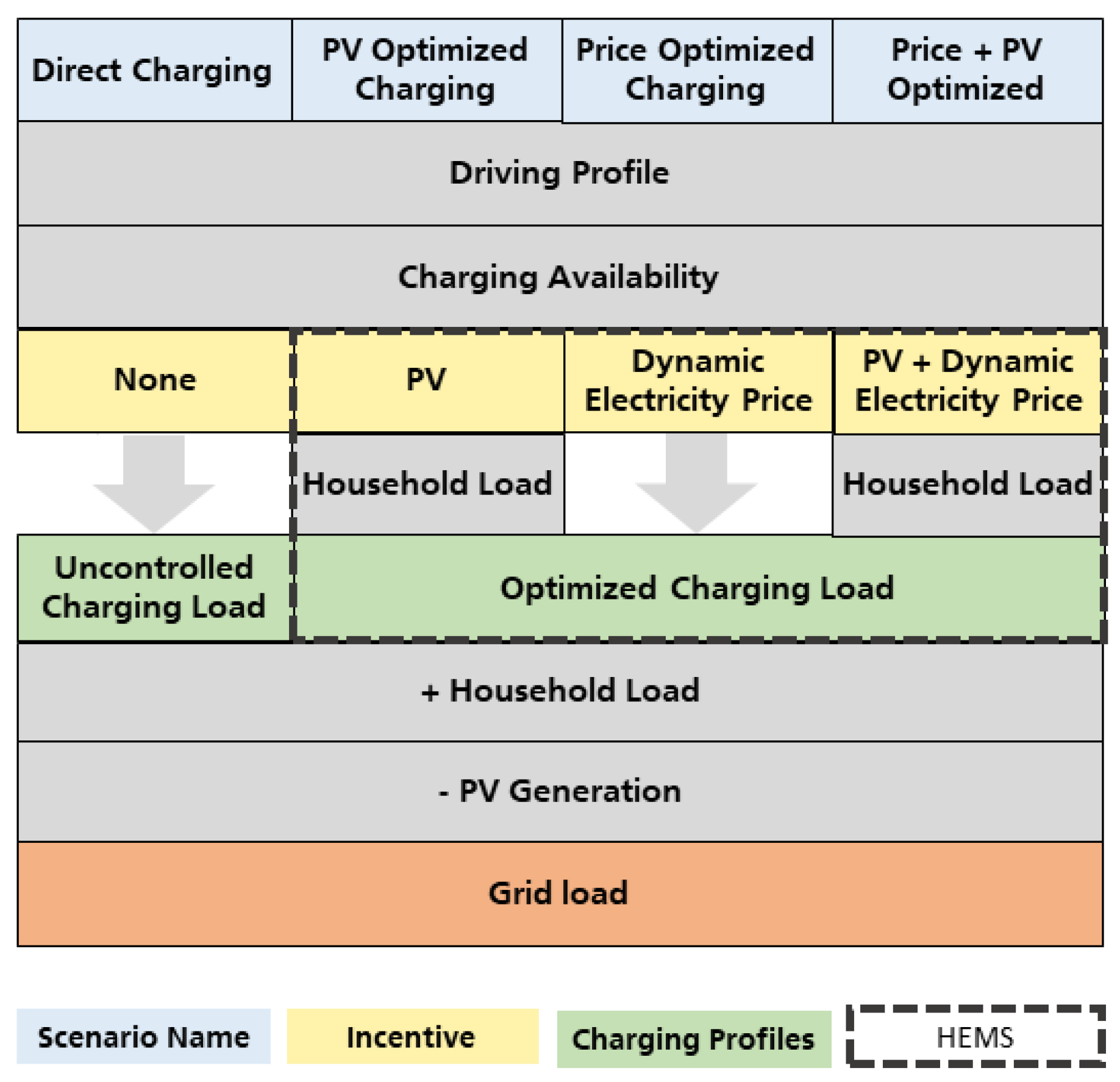
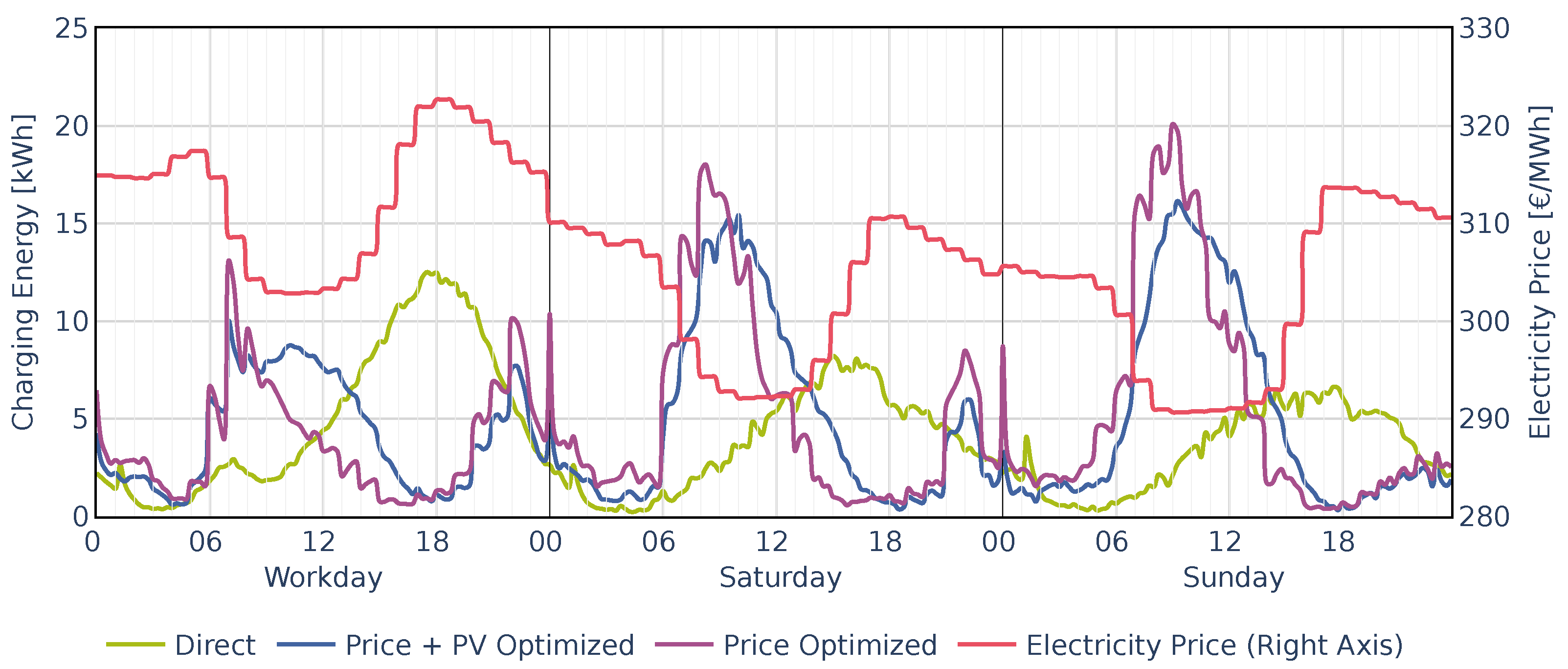
3.1. Charging Strategies

A total of four charging strategies are considered: three optimized and one uncontrolled charging strategy. Optimized charging involves having an HEMS in the home that uses different input signals to minimize charging costs. The input signals in this case are PV-generation and electricity price. In this study, optimized charging always refers to decentralized control without interaction or feedback between other households.

Uncontrolled charging is independent of these signals, and the user charges according to his preferences directly or only when the battery level is too low for the next trip.

The characteristics of the four charging strategies are described in

Table 1. Overview of the considered charging strategies.

Charging Strategy		Incentive	Description
Uncontrolled	“Direct Charging”	None	Users charge their car directly to the maximum capacity as soon as they arrive back home.
Controlled	”PV Optimized Charging”	PV generation	Users with a home PV system shift the charging process to maximize self-sufficiency while considering home demand.
	”Price Optimized Charging”	Electricity costs	Users directly receive the signal of the wholesale electricity prices and adapt the charging configuration to minimize electricity costs for charging.
	”Combined Price + PV Optimized Charging”	PV generation & Electricity costs	Users receive price signal of the wholesale electricity prices and adapt the charging configuration to minimize total household electricity costs.

.

The four charging strategies were tested on 100 households to also assess simultaneity effects. The households each have a PV-system, an EV, and a dynamic electricity tariff. In addition, the existing household load is taken into account. Figure 1 illustrates the considered household and their load flows.

The generation of the charging loads, as well as the load at the household grid connection point, is outlined in Figure 2. All four strategies are based on the driving profiles and charging availability; their generation will be discussed in Section 3.2. In the case of uncontrolled charging, the charging load profile can be generated directly from these (see left path in the graph). The second column of the graph shows the generation of the “PV optimized charging” scenario. In addition to the driving profile and charging availability, the PV generation and household load are also included here, as the household load competes with the EV for the PV energy generated. The input data is processed by an optimization program, whose design is described in Section 3.4. The charging time series optimized for maximum PV utilization is generated as a result. In the third case, a dynamic electricity tariff is used instead of PV in the optimization; the household load does not affect the optimization in this case. The fourth strategy is shown in the last column. Here, both PV and the dynamic electricity tariff are used as incentives. The optimization software decides which energy source results in the lowest charging costs at each point in time.

In order to not only be able to compare the charging loads but also to quantify the load at the grid connection point, the household load is added to the charging loads and the PV generation is subtracted from it. The resulting time series shows the grid load, which can be either positive or negative, in the case of PV feed-in.

3.2. Charging Profile Generation

Modeling of EVs essentially requires two input parameters as time series: energy consumption and location of the EV. How the energy consumption profiles for the EVs are created using mobility data and how the outside temperature affects this is described in this section.

3.2.1. Driving and Charging Profiles

Driving and charging profiles generation uses the data survey from “Mobilität in Deutschland 2017” [22] supplemented by traffic count data [23]. The survey includes data from people from around 150,000 households and contains trip data of a specific day as well as socioeconomic data from study participants. The data is used to create a time series in 15 min resolutions for a whole year for different region types and socioeconomic characteristics. In order to properly map the driving and charging configuration of car owners for each potential low-voltage network and to enable spatial allocation at the house level similar to that modeled in [24], households are differentiated into a total of 63 mobility groups according to the parameters in

Table 2. Categories for mobility groups (All combinations are possible).

Spatial Type
Urban	Rural
Metropolis	Central city
Bigger city	Urban area
Suburbia	Village area
Village area
Household
Net Income	Type
EUR < 2000	Single
EUR 2000–4000	Multi-person without children
EUR >4000 €	Multi-person with children

.

Within a mobility group, the driving configuration of the individual vehicles is statistically representative. This concerns, among other things, annual mileage, commuting configuration, and travel configuration. For instance, people with high income have longer commuting distances and more vacation trips than people with low income, whereas a car from a household with children only goes on vacation during holidays. Since a low-voltage network is always located within the same spatial type, combinations of up to nine different mobility groups, differentiated by household income and household type, can occur within a grid area. For a specific grid, the distribution can be chosen individually.

The driving profile is assumed as fixed so that the user can always make the trips without restriction due to battery capacity limits. The availability and power of charging capacity depend on the user preference to charge at home, at work, or in other places. The electrical consumption in kWh/km and the battery capacity are taken into account for each vehicle. The charging availability then forms a degree of freedom that can be used when creating the charging profiles by considering certain charging preferences, e.g., direct charging or optimized charging. As a result, charging profiles can then be derived depending on the preferences and habits of the vehicle owner.

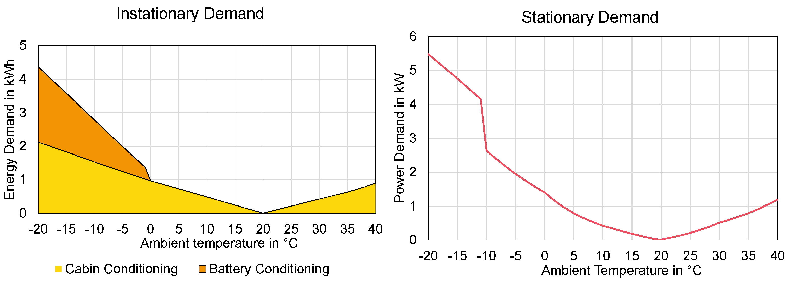
3.2.2. Impact of Temperature

Outside temperatures that deviate from the comfort temperatures of the vehicle user and place a particular strain on the battery result in temperature-related increased energy demand on particularly hot and cold days. This is especially important concerning distribution network considerations because there is a strong correlation with other temperature-dependent consumers and generators, especially heat pumps, which is relevant for the design of the networks. Temperature dependence distinguishes between steady-state and transient power demand. The steady-state power demand occurs when there is a balance between outside and comfort temperature while driving and energy must be supplied to the vehicle from the battery for heating/cooling. Figure 3 on the right-hand side illustrates the increased power demand of corresponding outside temperatures. The system’s power demand jumps from 2.95 kW to 4.65 kW below −10 °C due to the limited operating range of the EVs heat pump. In the temperature range between −10 °C and +40 °C, the electrical power demand behaves approximately symmetrically around the value of 20 °C.

The left-hand side of Figure 3 illustrates the transient additional power demand of a vehicle that arises from the heating of the vehicle cabin and the battery before driving and the energy required to precondition the battery.

The weather year 2012 was selected for the modeling because there was a particularly long cold period in this year, which represents an extreme situation for the system design. The additional demand is individual for each profile and depends on how many routes are driven on days with cold temperatures, and is about 10 to 15% above consumption for most profiles during the year. The additional demand applies equally to all motor vehicles within a network area and also affects other temperature-dependent electricity consumers such as heat pumps.

3.3. Input Data

This section describes the necessary input parameters. The basis for all charging strategies are the EV driving and presence profiles, whose generation is explained below, and also EV battery size and consumption. Additionally, all optimized charging strategies require PV, electricity price, and household load data.

3.3.1. Electric Vehicle

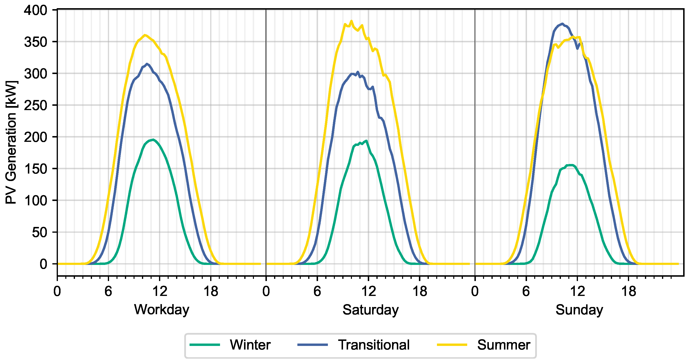
To represent the EV in the model, the driving profile, charging availability, minimum and maximum charging powers, energy demand, and storage capacity are needed.

For the case study, 100 driving profiles for metropolitan regions are chosen. Figure 4 shows the minimum, median, and maximum movement per quarter-hour for the 100 aggregated profiles. It shows, for example, that the aggregated vehicle pool travels a median of about 50–75 km per quarter-hour between 6 a.m. and 6 p.m. on workdays, which corresponds to 24 to 36 km per vehicle in this period. The average annual driven distance equals 11,600 km. The minimum and maximum driven distances are 1700 and 48,000 km, respectively.

The time series with charging availability is used to determine the periods at which the EV is parked at home and could be connected to the electricity grid, to be available for the charging process (referred to as presence). It is assumed that the connection with the home network is established immediately after the arrival of the EV and is not disconnected until the next trip. The binary charging availability is multiplied by the maximum charging power. The aggregation of these profiles results in a maximal possible charging power for the EV pool shown in Figure 5. The lower red dashed line shows the maximum load that could occur on any day of the year, while the values of the upper dashed line may occur only on individual days of the year. The 0.25 to 0.75 quantile is shown with the light blue area around the mean. Since it is assumed that each EV is connected to the house network through a 11 kW wallbox, the absolute maximal possible charging power of the aggregated pool is hence 1100 kW and could only occur during night between 11 p.m. and 6 a.m., when apparently all EVs are at home. Due to the requirement of at least 6 A charging current, the minimum charging power of each individual EV is 1.4 kW.

In addition to the time series described, EVs are also characterized by their consumption and storage capacity.

Table 3. Overview of characteristics and amount of EVs [25].

Type	Capacity [kWh]	Consumption [kWh/km]	Qty.
BEV small	35.00	0.16	28
BEV small (second car)	25.00	0.16	11
BEV medium	60.00	0.20	28
BEV medium (second car)	50.00	0.20	1
BEV big	80.00	0.25	9
BEV light utility vehicle	45.00	0.28	4
PHEV small	8.80	0.16	1
PHEV small (second car)	8.80	0.16	1
PHEV medium	11.50	0.20	12
PHEV medium (second car)	11.50	0.20	5
Total Quantity			100

shows the attributes of the modeled EVs and their frequency of occurrence (qty) in the aggregated pool as it was derived from stakeholders’ assumptions in [25]. The compilation was randomly chosen from a bigger set of profiles which represents today’s proportion of vehicle sizes and a proportion between BEV and PHEV according to a bottom-up consumer demand model [26].

The spatial perspective of the study relates to metropolitan regions. As described in Section 3.2.1, the driving profiles contain a large amount of metadata. In order for the driving profiles to match the spatial type, the data was filtered according to household income and household type (compare Table 2) and a composition that was representative of metropolitan regions was selected. Figure 6 shows this distribution. Here it can be seen, for example, that slightly more than half of the profiles are in the lower income bracket and that 20 profiles correspond to the behavior of singles.

3.3.2. Photovoltaic

The PV time series model developed at Fraunhofer IEE was used to generate PV generation time series [27]. The PV time series model is a physical model that uses meteorological data as input to represent the generation of electricity of a PV system.

To calculate the optimal PV system size considering the household and EV load, an investment model was used [28], which extends the deployment model described in Section 3.4 with investment parameters such as investment costs, operating costs, and discount factor. For the PV system, EUR 900/kWp was assumed for the investment cost, and 2.5% of the investment amount per year for the fixed operating costs. The internal rate of return was assumed to be 3%. The resulting average size of the PV rooftop systems for all 100 households is $8.2$ kWp. The smallest system has a maximum power of only $3.0$ kWp and the largest is rated at $19.6$ kWp; the sum of all 100 PV systems is 818 kWp.

It is assumed that the households may be distributed throughout the country, so there were PV time series for nine different locations in Germany used: Berlin, Hamburg, Cologne, Frankfurt, Stuttgart, Duesseldorf, Leipzig, Dortmund, and Hanover. For every location, three time series are generated, each with a different orientation of the roof surface: south, southwest, and southeast. This means that a total of 27 different PV generation profiles are included, distributed evenly among the households so that each profile occurs about three times.

Figure 7 shows the mean PV generation of all 100 systems for different type days and seasons. The PV time series are based on the 2012 weather year.

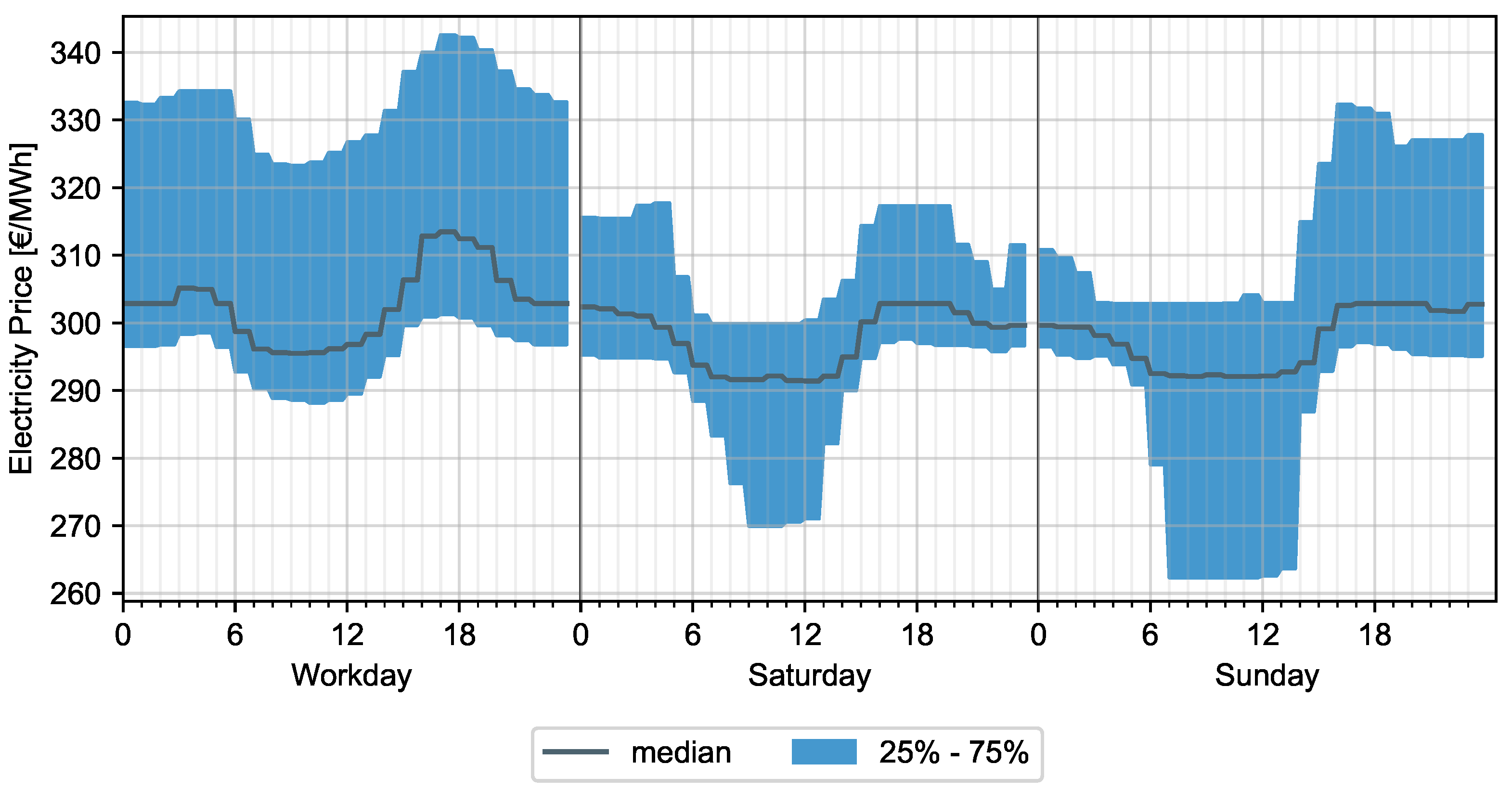
3.3.3. Dynamic Electricity Price

The charging strategies “price optimized charging” and “combined price + PV optimized charging” receive a dynamic market-driven electricity price, based on the hourly prices of the day-ahead market of the electricity exchange. To reflect an energy system with a significantly higher share of renewable energy sources as it is expected in 2030, no historically day-ahead time series are used, but instead it was generated using the wholesale market simulation developed by Fraunhofer IEE [29]. The fixed price components common in Germany were added, which include grid charges, surcharges, and taxes. An overview of the resulting dynamic electricity price per day type is illustrated in Figure 8.

The average of the annual series for the dynamic electricity tariff is equal to EUR 310/MWh and the daily mean volatility (standard deviation) is 9.8 and the annual volatility is 27.5. It is assumed that electricity generated by PV is less expensive than electricity purchased from the grid, and is preferentially used for household and charging loads.

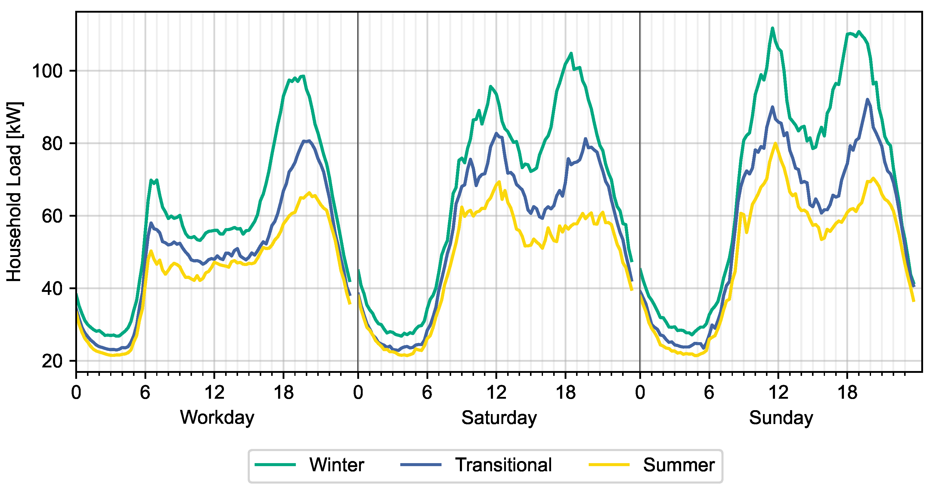
3.3.4. Household Load

A total of 74 different household load profiles are considered, published by HTW Berlin [30]. Since 100 households are considered in this study, profiles 1 to 26 occur twice. Figure 9 shows the average electrical load of all 100 households (aggregation of all 100 load profiles) grouped per day type.

The annual electricity demand of households ranges from 1394 to 8544 kWh, and the average electricity demand is about 5200 kWh. The shape of all profiles correlates very well with the standard load profile [31].

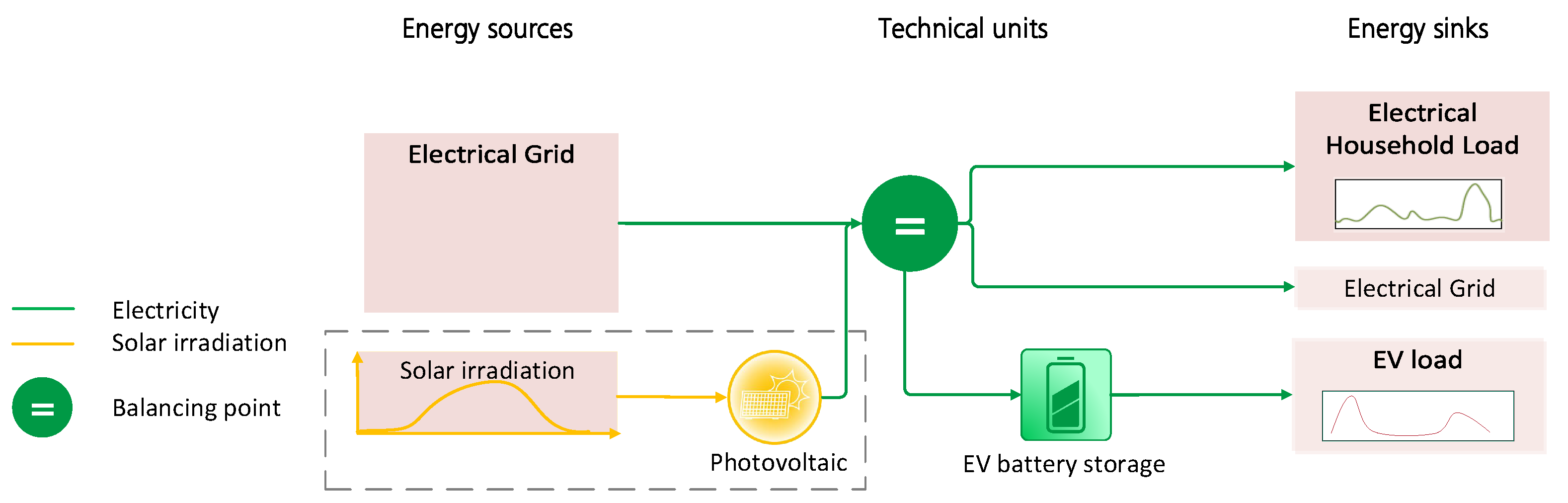
3.4. Optimization Model

This section describes the methodology for the economic optimization. The considered system to optimize here is a household that has a desire to reduce its total electricity consumption costs. To achieve this goal, it is assumed that the households have an HEMS that can optimally distribute energy within the household. The HEMS is simulated using a mixed-integer linear optimization program that controls the operation of the flexible loads. As a result, it provides the unit commitment problem time series and, therefore, in this particular case, the charging time series for the different optimized charging strategies. The model considers the technical and economic constraints of energy generation, consumption, and storage units. The objective function maximizes the economic gains over the solution space. Each individual household is optimized independently, there is no dependency or feedback to other households.

Due to the inaccuracy associated with forecasting and optimization over a long time interval, a rolling horizon framework is adopted here to solve the addressed problem iteratively in a finite-moving-horizon of time intervals. Precisely, the entire time horizon of 1 year is separated into equal time intervals of 2 days and the optimization problem is expressed and solved at each rolling step over the prediction time horizon, but only the solution of the first day in each step is employed. Then the forecasting horizon is shifted by 1 day forward and the calculation is reiterated for the new rolling horizon until the end of the entire simulation period (1 year in this case). The ultimate decisions are the sequence of decisions met on the first day of each optimization step.

Figure 10 visualizes the modeled optimization system. It includes one or two energy sources, depending on the case study. One energy source represents the electrical energy from the electrical grid, and the second represents the electricity generated by PV. It also contains two energy sinks, one for the household demand and one for the EV demand. Household and EV load profiles are assigned to the sinks, specifying the amount of energy required at each time step of the simulation. The energy demand of the EV is supplied from the EV storage, which is also modeled. The time series for the charging availability controls which times the EV storage is connected to the local household grid, and therefore can be charged.

In the following part, input parameters are marked with a capital letter, and variables that are a result of the optimization are marked with a small letter.

The objective function maximizes the overall profits of the households, which considers income from grid feed-in, costs of the operation of the energy units, and electricity taken from the grid, as seen below:

$$maximizing\sum _{t\in T}\left(p_{\mathit{feed}-\mathit{in},t}^{grid}·{\rho }_{\mathit{feed}-\mathit{in},t}-p_{\mathit{cons},t}^{grid}·{\rho }_{\mathit{cons},t}-s_t^{comfort}·{\rho }_{\mathit{comfort}}\right)·{\Delta }_T$$

(1)

where $p_{\mathit{feed}-\mathit{in},t}^{grid}$ is the power flow going to the grid, $p_{\mathit{cons},t}^{grid}$ is the grid consumption power, and $({\rho }_{\mathit{feed}-\mathit{in},t},{\rho }_{\mathit{cons},t})$ are the prices for electric energy fed into or taken from the grid, respectively. $s_t^{comfort}·{\rho }_{\mathit{comfort}}$ represents a penalty term that provides an incentive to achieve a comfort SoC as quickly as possible, see Equation (8) for a more detailed description.

The PV system is in each time step t ($P_t^{pv}$) constrained by a minimum generation of 0 and the forecasted generation ($P_{fc,t}^{pv}$) described in Section 3.3 as input time series:

$$0\le p_t^{pv}\le P_{fc,t}^{pv}$$

(2)

The EV storage is defined by the charging/discharging power and the SoC for each time step ($e_t^{ev}$). The SoC at time t ($e_t^{ev}$) is calculated by subtracting the losses during ${\Delta }_t$ and the discharged energy at time t ($P_{discharge,t}^{ev}$, Domain ${\mathbb{R}}_0^{+}$) by the previous period’s SoC ($e_{t-1}^{ev}$) and adding to that the charged energy at the same time ($P_{charge,t}^{ev}$, Domain ${\mathbb{R}}_0^{+}$), which is taken from the grid or from PV, such that

$$e_t^{ev}=e_{t-1}^{ev}·(1-{\mu }_{time}^{ev}·{\Delta }_t)+\left((1-{\mu }^{ev})·p_{charge,t}^{ev}-(1-{\mu }^{ev})·p_{discharge,t}^{ev}\right)·{\Delta }_t$$

(3)

where ${\mu }_{time}^{ev}$ defines the energy loss over time, while ${\mu }^{ev}$ indicates the energy losses during charging and discharging processes.

The SoC at any time step is constrained by minimum and maximum SoC:

$$e_{min}^{ev}\le e_t^{ev}\le e_{max}^{ev}$$

(4)

Charging rates are limited by the maximum output capacities of the wallboxes $P_{wallbox,o}^{ev}$. These rates are also constrained to positive values. This is presented in Equation (5).

$$0\le p_{charge,t}^{ev}\le P_{wallbox,o}^{ev}$$

(5)

The energy sources are used to supply energy to the optimization system. While the energy yield of the PV system is covered by Equation (2), the electricity consumed from the grid is flexible and dependent on the self-generated electricity and household load. No additional constraints are accordingly required.

The energy balance here is ensured by two balancing equations. One defines the relationship within the household’s local electricity grid. The PV generation $p_t^{pv}$ and energy purchase from the grid $p_{cons,t}^{grid}$ are equal to the charging of the EV $p_{charge,t}^{ev}$, the household load $P_t^{el}$, and the feed-in of surplus PV to the grid $p_{feed-in,t}^{grid}$; compare Equation (6).

$$p_t^{pv}+p_{cons,t}^{grid}=p_{charge,t}^{ev}+P_t^{el}+p_{feed-in,t}^{grid}$$

(6)

The second balancing equation defines the relationship between EV storage and EV consumption $P_t^{ev}$, as it is shown in (7).

$$p_{discharge,t}^{ev}=P_t^{ev}$$

(7)

The free charge control by the HEMS is limited below a SoC of 40%. It is assumed here that users want to reach a minimum Soc of 40% as quickly as possible due to comfort features. This is integrated into the economic model via a virtual penalty, which is due below the comfort level. If the current Soc ($e_t^{ev}$) is below the comfort SoC ($e_{comfort}^{ev}$), the left part of the inequality (8) becomes negative. This forces the binary variable ($s_t^{comfort}$) to become 1 so that the inequality remains valid. The binary variable is included as a cost in the objective function and thus leads to a penalty for falling and staying below the comfort level. In the objective function, the binary variable is multiplied by the number ${\rho }_{\mathrm{comfort}}$ whose magnitude can be used to influence the intensity of the effect.

$$e_t^{ev}/e_{max}^{ev}-e_{comfort}^{ev}/e_{max}^{ev}\ge -s_t^{comfort}$$

(8)

Respecting the constraints shown in this section, the optimization system can freely decide when and how much energy would be feasible and reasonable to use from the grid and if the energy generated by the PV system is fed into the EV storage, household, or the grid. Moreover, it can also choose the SoC of the EV storage as far as it is connected to a charging station. The most important result of the optimization is the charging time series which will be analyzed in Section 4 and referred to as optimized charging configuration.

The constraints described above, as well as the objective function, were implemented with the open-source modeling framework Pyomo [32] and, together with the input parameters, resulted in the micro-economic optimization.

4. Results

The following section outlines the effect of different charging use cases, the resulting costs for households, and their implications for simultaneity with other household loads and PV generation. Section 4.1 shows general effects of electricity price and PV incentive on charging configuration. However, for local low-voltage grids it might be more relevant to see when the highest charging peaks occur. Hence, Section 4.2 presents the occurrence and extent of the highest common charging peaks for the configurations. Moreover, in Section 4.3, an outlook on what different charging configurations mean for the household electricity costs is given. However, for grid considerations, other decentral consumers have to be considered. Therefore, Section 4.4 considers also the household load and takes the aggregated configuration of decentral consumers in terms of simultaneity and charging peaks into account.

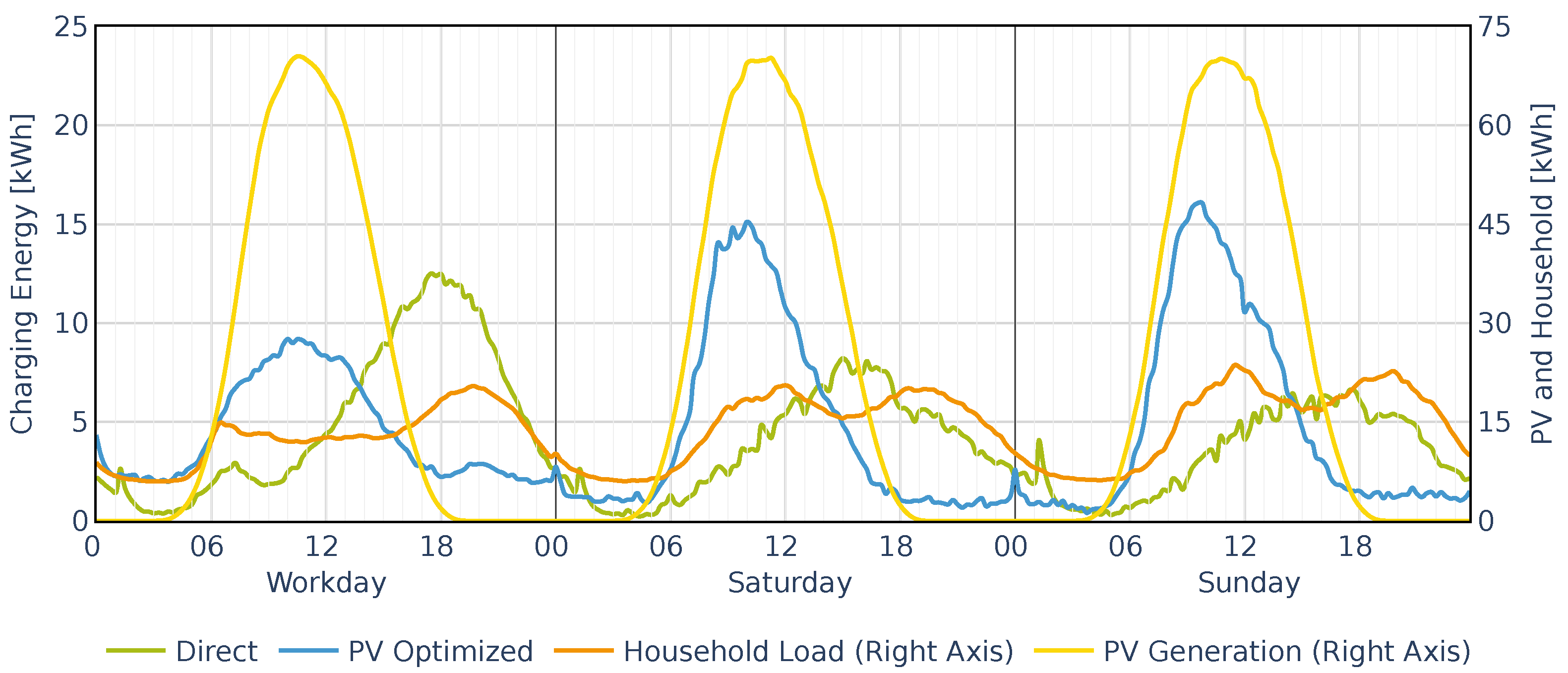
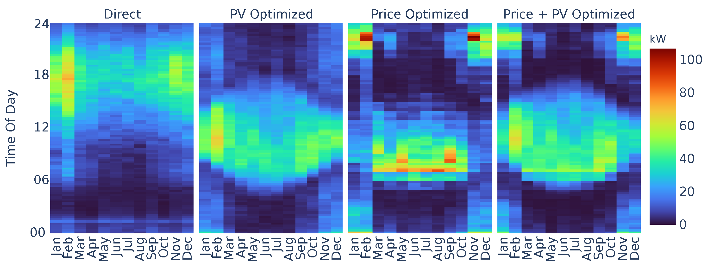
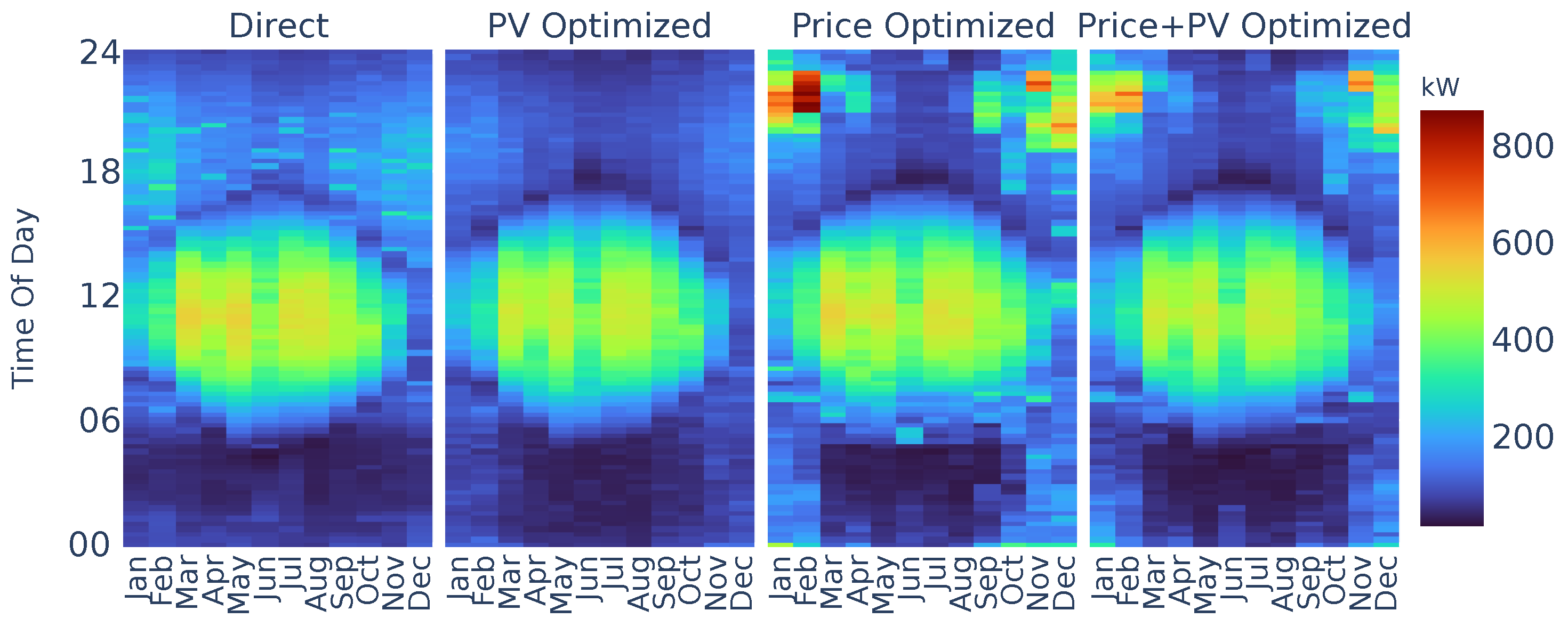
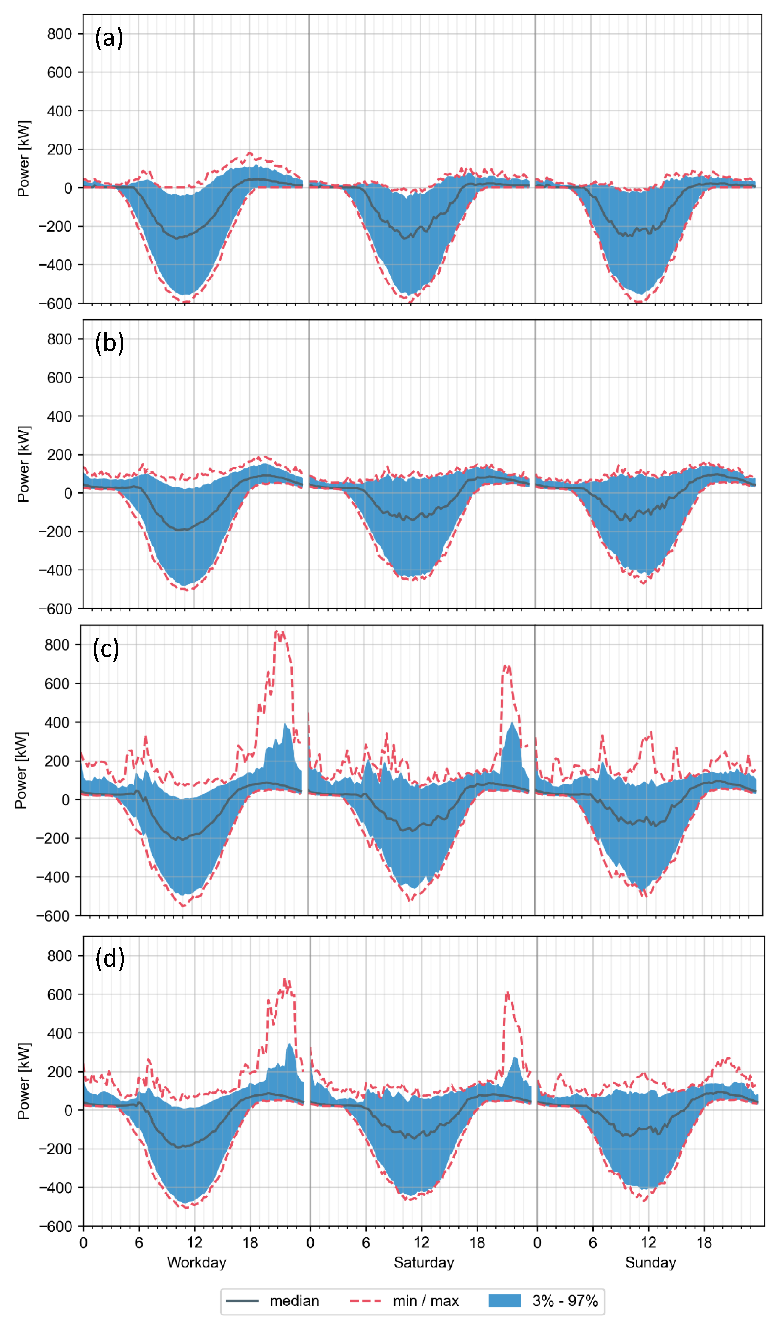
4.1. Effects of Optimized Charging Configurations on Load Shifting

Figure 11 illustrates the charging configuration for 100 vehicles comparing “direct charging” against “PV optimized charging”. It shows how well “PV optimized charging” adapts to the PV generation for the average type days. The “PV optimized charging” profile fits the PV generation profile although PV plants are often generating, while EVs are driving. On weekends, the effect is even stronger and an even higher share of charging power can be shifted into times with high PV generation. This means that the battery storage capacity of EVs is large enough to facilitate shifting of charging power flexibly throughout the day and also from workday to weekend. The PV incentive shifts the charging process away from the household load peak in the evening in workdays.

Figure 12 compares “direct charging” with “price optimized charging” and “combined price + PV optimized charging”. Again, it shows that there is enough flexibility for the optimization to move most of the charging energy into low price times on the weekend, late evening, or in the morning. “Combined price + PV optimized charging” presents a mixed incentive scheme of the electricity price, PV generation, and household load. This combined charging strategy shifts some of the charging load into daytime with high PV generation and some of the charging load into low price times.

Figure 13 shows the average of charging power for each month and time of day.

In case of “direct charging”, most of the charging processes take place in the second half of the day between 12:00 and 21:00. The behavior remains similar throughout all seasons but is stronger in winter especially in the cold month February, which for the contemplated weather year 2012 is the coldest month.

Users with own PV plants (“PV optimized”) charge mainly during daytime. The seasons affect this in a way such that in winter months the charging processes concentrate more on hours during the day around noon. In winter you can also find more charging processes in the late afternoon and morning hours.

As far as the configuration “price optimized charging” is concerned, the distribution of load peaks corresponds to the course of the electricity prices. In the winter months between November and February, charging occurs mostly in the morning before 10:00 a.m., while in summer and transition seasons, charging is shifted to noon and this can be justified by the integration of PV which, with high generation, may reduce the price of electricity.

The charging strategy of “combined price + PV optimized charging” has the characteristics of two single configurations, while the characteristic of “PV optimized charging” is being dominant. Due to reduced solar radiation in winter, EVs on grid are charged at night when the electricity price is low.

In summary, the configuration “price optimized charging” has the highest concentration of charging processes at specific times. In contrast, the configuration “PV optimized charging” has the lowest aggregated charging power, and charging time is more evenly distributed throughout the day. Compared to other configurations, the configuration “direct charging” starts earlier and is less affected by seasons with charging concentration in the coldest month February.

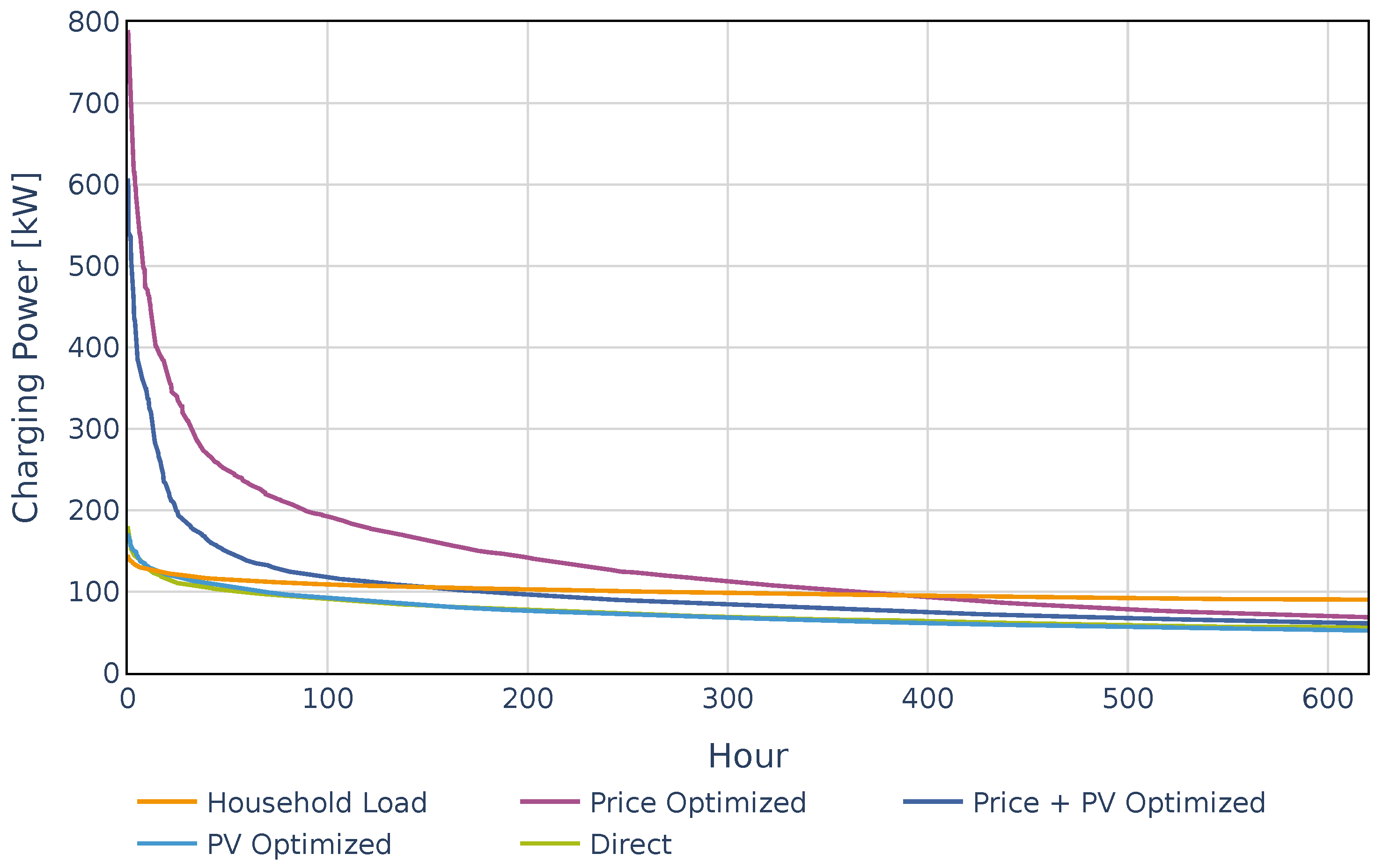
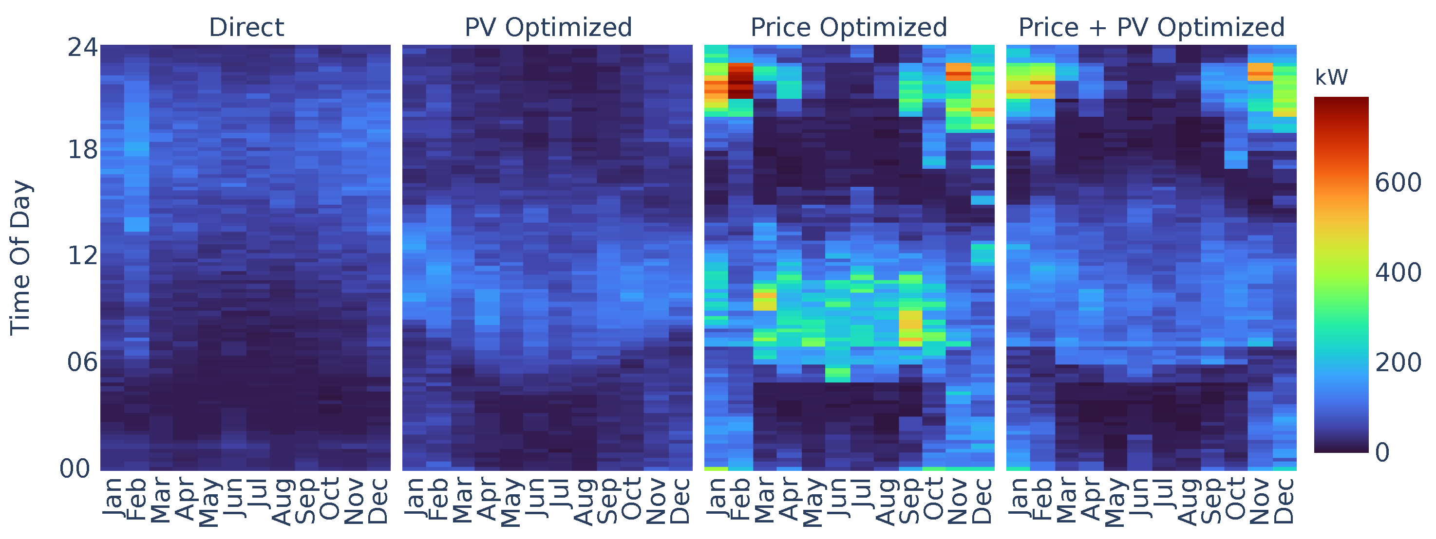
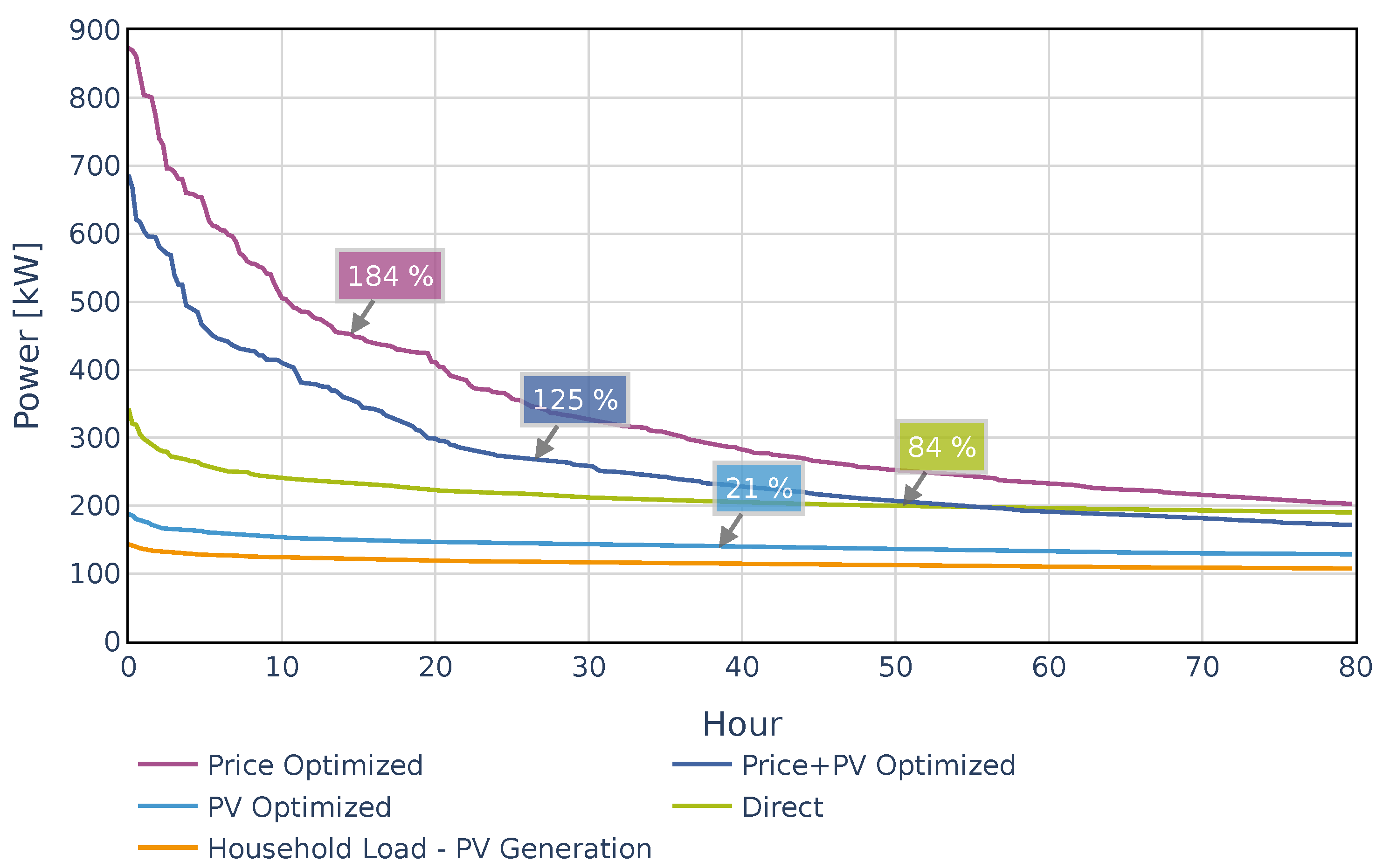
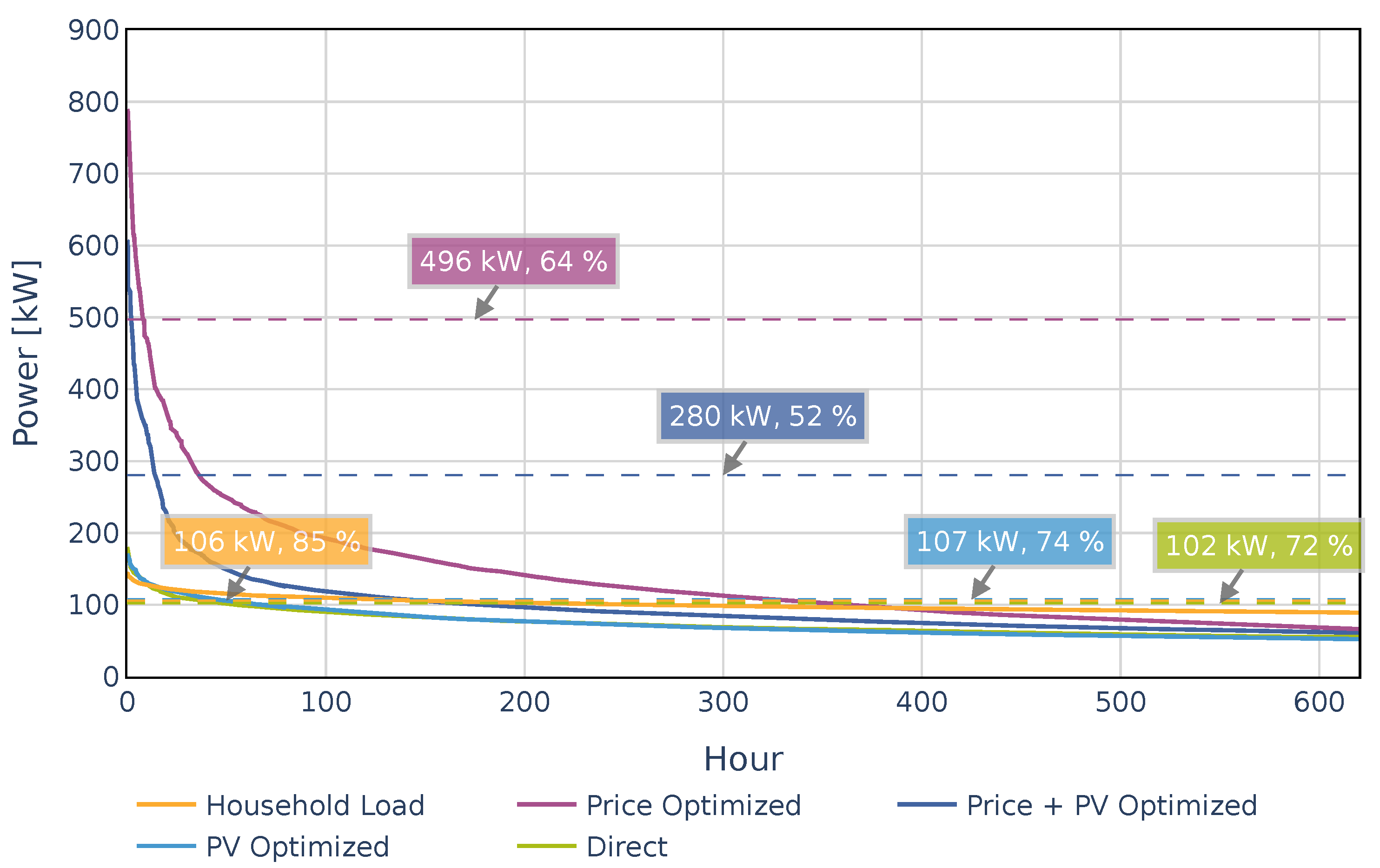
4.2. Occurrence and Extent of Charging Peaks

Besides the average configuration of each charging configuration, it is important to know what the maximum of charging power is and when it occurs. Therefore, Figure 14 shows the maximum charging power for each month and time of day for each charging configuration.

Moreover, it shows the highest concentration of charging processes being at the same time as in Figure 13 but more focused on fewer hours per day. Here, it can be noticed that the “price optimized charging” has the highest aggregated charging values followed by “combined price + PV optimized charging”, while the maxima of “direct charging” and “PV optimized charging” are much lower and hardly visible in this illustration.

The impact on aggregated peaks is illustrated in Figure 15.

Firstly, it can be seen that the maximum aggregated power of the household load lies at almost 150 kW. The peaks of the “direct charging” and “PV optimized charging” configurations are similarly high at 200 kW. It can be noted that the highest peaks occur for the “price optimized charging” with the peak being at almost 800 kW. “Combined price + PV optimized charging”, on the other hand, has a lower, but still very high, peak at around 600 kW.

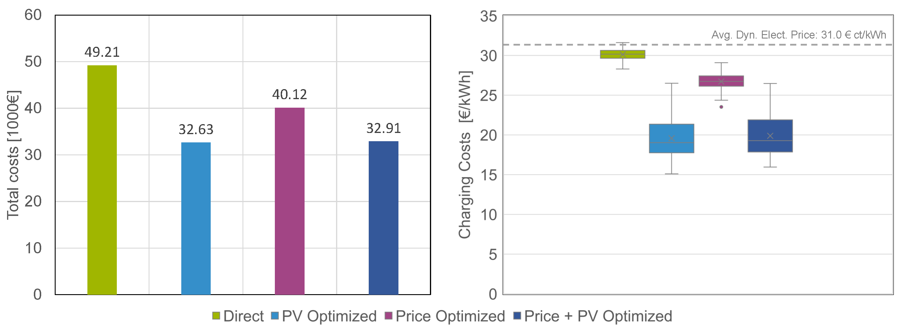
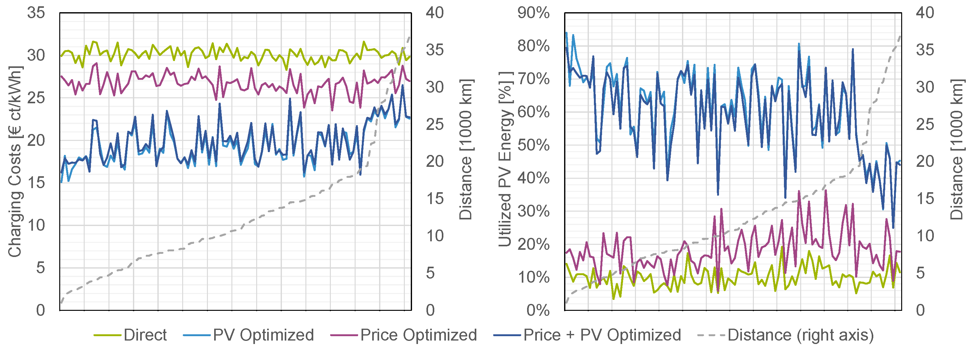
4.3. Economical Aspects on Households

This subsection of the paper discusses the economic aspects correlated to the previously discussed charging configurations of the EV users. The economics of EV charging can be assessed by evaluating the costs and benefits, which could involve different stakeholders, technologies, and parameters. In this study, however, only the costs of charging are to be assessed, considering a comparison between the different charging configurations. In order to have comparable results, in terms of charging electricity prices and total costs, the utilization of PV energy was incorporated and prioritized for charging the EVs over covering the household load for the calculations of “direct charging” and “price optimized” strategies.

Figure 16 consists of two subplots; on the left side, the total charging costs are illustrated for the 100 aggregated charging profiles, over the simulation year and per charging configuration. Here, the total costs were calculated by multiplying the hourly electricity price by the quarter-hourly electricity consumption. In this context, the highest total costs are depicted for“direct charging”, while the most economical option is the “PV optimized charging” with a difference of 33.7%. The (“price + PV optimized charging” has a slightly higher total cost than the “PV optimized”, with a percentage of 0.8%. Accordingly, “price optimized” represents the third most economical option with a variation of 18.5% compared to “direct charging”. For these calculations, a EUR 6 ct/kWh is adjusted for each of the levelized cost of electricity (LCoE) and the opportunity costs (in total: EUR 12 ct/kWh) of the PV-generated electricity and utilized for charging. The opportunity costs here, express the lost profit that might be generated by feeding the PV-generated electricity in the grid.

Subsequently, the right side of Figure 16 shows the distribution of charging electricity costs in EUR ct/kWh for each charging configuration. It can be noted that PV integrated optimization strategies are more feasible and have more economic benefits than the “price optimized” and uncontrolled strategies. Within this framework, “direct charging” represents the highest average cost of electricity, with EUR 30.1 ct/kWh which keeps it below the average dynamic electricity rates used in these simulations of EUR 31.0 ct/kWh (represented by the dashed line on the same figure). This is mainly due to the utilization of PV energy in these calculations.

In comparison to that, all optimized charging configurations showed lower prices with an average of EUR 26.7 ct/kWh, EUR 19.9 ct/kWh, and EUR 19.6 ct/kWh for “price optimized”, “price + PV optimized charging” and “PV optimized” charging configurations, respectively.

To have a better insight into the cost of electricity for each charging configuration, Figure 17 is plotted and arranged in an ascending order referring to the driven distance in kilometers per EV for all of the 100 EV profiles (interpreted on the x-axis). As it can be seen on the left subplot, the cost of electricity for PV-integrated optimized strategies are almost the same or lower than other charging strategies for all driven distances. It can also be noted that cars with a higher driven distance do not cause higher charging costs for “direct charging” and “price optimized charging”, while the PV-integrated optimized strategies are directly proportional to the driven distance. This trend can be clarified by exhibiting the subplot on the right side, as the share of PV-generated electricity is lower for cars with a higher driven distance. This is mainly due to the flexibility the EV users have when driving less. For “direct” and “price optimized” charging, it is not the case due to the low utilization of PV energy that is bound between 3–36% with an average of 14%, compared to 25–84% with an average of 60% for “PV optimized” and “price + PV optimized” charging strategies. As a conclusion, incorporating a PV optimization strategy would increase the employment of PV energy for charging by 46% on average.

Consequently, “PV optimized charging” shows the lowest cost of charging electricity followed by the “price + PV optimized charging” and then the “price optimized charging”. All three optimization strategies show an economical benefit over the uncontrolled charging configuration.

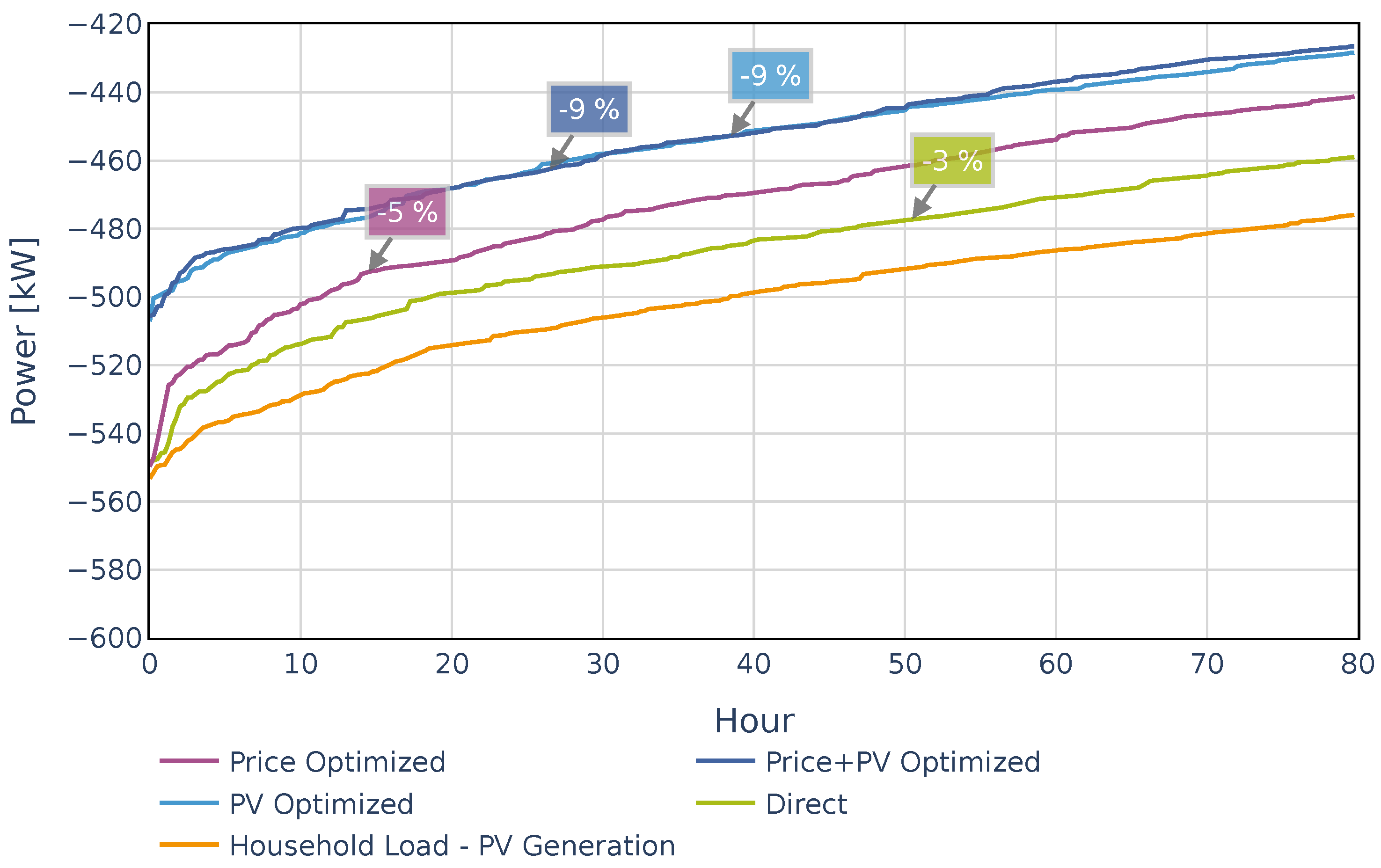
4.4. Effect on Grid Load Considering Aggregated Configuration with Household Load

The maximum grid load can happen in both cases: High electricity consumption with low PV generation or low consumption during times of high PV generation. For a better understanding of the impact that the charging configurations could have on the grid, the combined load of households and EV charging is considered. Figure 18 illustrates grid load, which is in this study defined as the maximum of the aggregated charging power and the household load minus the PV generation as it is shown in Equation 9:

$$Gridload=|EVload+Householdload-PVgeneration|$$

(9)

The result looks similar to Figure 13. The PV generation for any household with PV causes the highest peaks during daytime.

The sizing of lines and transformers in an electrical grid is dependent on the expected maximum loading. Therefore the 1 % maximum values of the grid load are looked at in more detail. Figure 19 depicts the sorted grid load together with the household load and zooms into the 1% largest values. The lines show the highest 1% of the grid load, aggregated over all 100 systems. In comparison, the household load without any EV charging power is shown. The text annotations show the factor by which the grid load is increased by the charging power compared to the household load minus PV for the largest 1% of values.

“Direct charging” without any optimization increases grid load by 84%. In the case of “PV optimized charging”, the additional grid load for charging EVs is comparably low (+21%). The most remarkable increase of 184% occurs for the “price optimized charging”. For “combined price + PV optimized charging”, the peak load more than doubles and increases by 125%.

In electrical grids higher load causes a fall of the voltage and higher generation causes an increase of the voltage. The voltage needs to stay within maximum and minimum limits. If this cannot be guaranteed grid reinforcement or voltage regulation components needs to be invested. In Figure 20, the sorted grid load is presented again but taking the highest negative value for grid load. This presents the case of higher generation.

The aggregated grid load “PV optimized charging” and “combined price + PV optimized charging” in this case decreases by 9%. If PV is not an optimization incentive, the decrease is smaller and lies at 3% for “direct charging” and 5% for “price optimized charging”. At this point, it should be mentioned that not necessarily every household with an EV also has a PV plant. This study intends more to display how much simultaneity of EV, PV, or electricity prices affects the grid load.

Figure 21 shows the statistical distribution of the grid load of the four charging strategies and each type day. The light blue area shows the values between the 3% and 97% quantile. The figure illustrates at what times of day and days of week high loads can occur. Subfigure (a) shows the uncontrolled case with moderate load peaks with a maximum positive value of 200 kW. It also shows that feed-in from PV regularly causes a high negative load of about 600 kW, which is higher than in all optimized scenarios. In subfigure (b), the “PV optimized charging” strategy is illustrated. It shows a similar profile for the positive load side, as shown in (a), but compared to (a), the maximum negative load is 150 kW lower on weekdays and about 200 kW lower on weekends. This clearly shows a beneficial effect on the grid load due to PV-optimized charging. Subfigure (c) for the “price optimized charging” scenario shows extreme positive peak loads with more than 800 kW, especially at night. Here, the different characteristics between working days and Saturdays and Sundays become even more apparent. The partly very high distance between the light blue area and the red dashed maximum line at some times of day indicates how infrequently the high charging rates occur. The scenario “combined price + PV optimized charging” in subfigure (d) shows also high positive peak loads up to 600 kW in some cases, but not as high as (c). Scenarios (c) and (d) clearly show that the identical price signal for all EVs, which serves as an incentive to shift charging power to times when electricity is low-priced, can lead to high simultaneity and thus cause high load peaks in particular cases.

To see what potential there might be for interventions on the grid level, the dashed line shows how much the maximum aggregated charging power can be reduced, assuming that 3% of the energy can be shifted. The potential for grid-related reduction measures is illustrated in Figure 22.

For “price optimized charging”, the peak could be reduced by 36% to 496 kW. For “combined price + PV optimized charging”, the peak can be reduced even more, by 48%, to 280 kW after cutting off 3% of energy.

5. Sensitivity Analysis

This section reflects the robustness of the results towards some basic assumptions that might change in future.

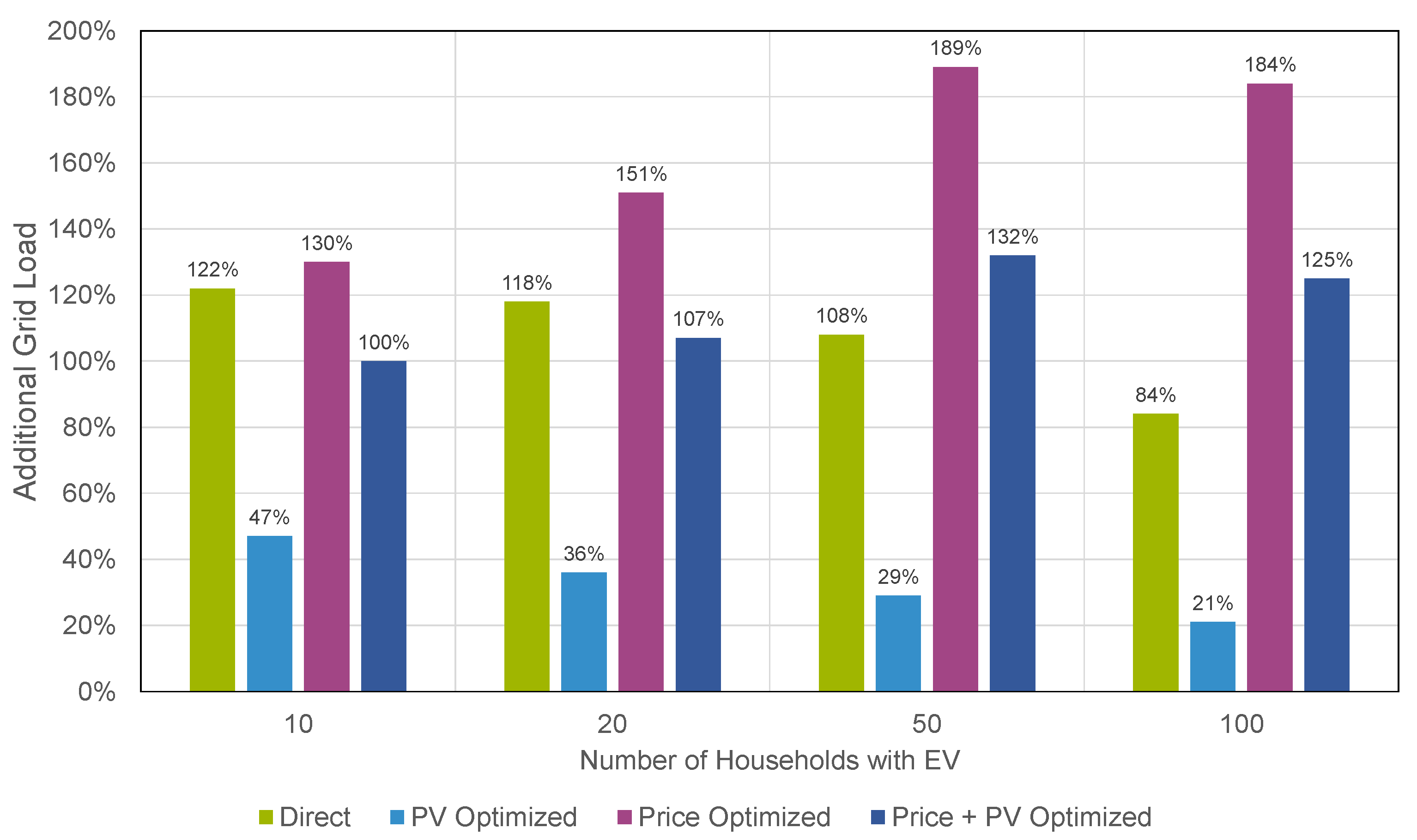
5.1. Number of Households and EVs

The effect on additional grid load by 100 households and EV charging profiles is compared to the impact on grid load with fewer households and EVs. Figure 23 shows the largest 1 % values of additional grid load caused by a different number of EVs in the sample.

Although the sample size is not very high and more repetitions of sampling could validate the results better, a clear tendency can be deduced. For configurations that do not include equal price incentives, such as “PV optimized charging” and “direct charging”, the additional grid load decreases with the number of profiles, whereas those configurations that use the electricity price as incentive have an increasing relative impact on grid load which might be asymptotic at some point.

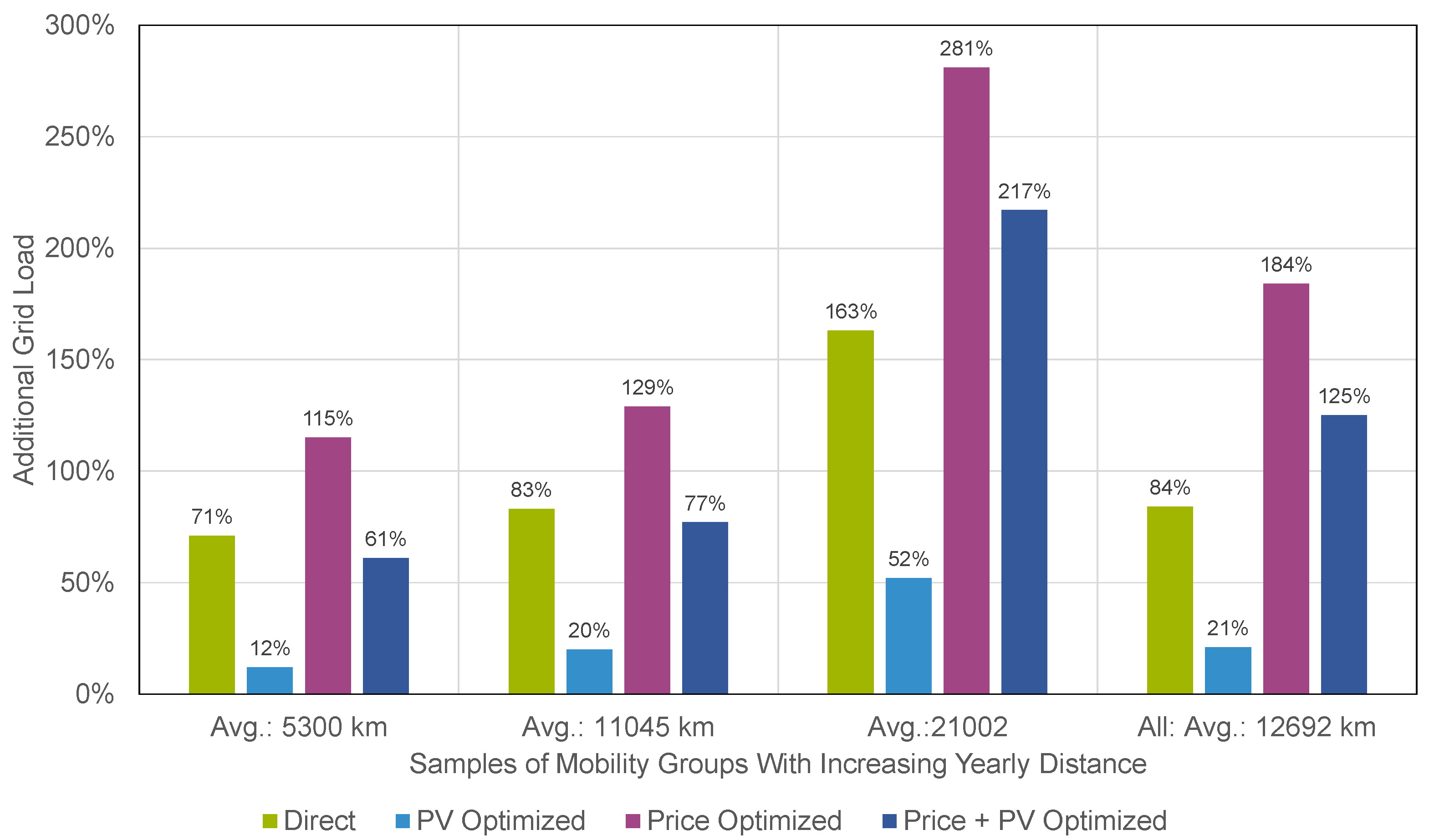
5.2. Yearly Driven Distance

Cars with a higher distance consume more energy and are consequently expected to cause higher additional grid load. Figure 24 quantifies this effect. The sample used in previous sections with 100 profiles is sorted by yearly driven distance and split into three groups with the same number of profiles.

The smallest group drives 5300 km per year on average and would cause an additional grid load of 71% for “direct charging”, 12% for “PV optimized charging”, 115% for “price optimized charging”, and 61% for “price and PV optimized charging”. For the second group, with an average of 11,045 km yearly distance, the additional grid load increases only slightly, whereas the additional grid load for the third group increases stronger and is especially strong for the controlled charging configurations. As a conclusion, it can be seen that number of EVs inside a grid area has a huge impact on the challenges faced.

5.3. Electricity Price Volatility

Due to several factors, including political, economical, and technological, while considering the developing penetration of renewable energy, a higher volatility in electricity market prices is expected in the upcoming years [33]. As a consequence, synthetic price time series with higher volatilities and standard deviations of EUR 55 and 108 ct/kWh were generated by integrating an incremental factor ($I_F$) of 2 and 4, respectively, in Equation (10) to see the impact of different EPEX day ahead market prices.

$$S_{EP}=(EP-Avg\left(EP\right))*I_F+Avg\left(EP\right)$$

(10)

where EP is the consumers’ electricity prices, and $S_{EP}$ represents the synthetic electricity prices that consider the $I_F$. Here, however, Equation (11) is applied to avoid outliers including very high peaks and low valleys, and to keep the synthetic electricity prices in a plausible range.

$$-300€/MWh<EP-Avg\left(EP\right)<+300€/MWh$$

(11)

The implied volatility revealed much better economic characteristics for the “price optimized charging configuration, especially at an $I_F$ of 4. In contrast, “direct charging” and “PV optimized charging” experienced a negative impact. This has kept the “price + PV optimized charging” at an almost constant level.

Table 4. Economical aspects while considering different incremental factors.

Charging Configuration	Reference at ${\mathit{I}}_{\mathit{F}}$= 1	Volatility at ${\mathit{I}}_{\mathit{F}}$= 2		Volatility at ${\mathit{I}}_{\mathit{F}}$= 4
	Total costs [EUR 1000], Avg. Charging costs [EUR ct/kWh]	Total costs [EUR 1000], Avg. Charging costs [EUR ct/kWh]	+/− [%]	Total costs [EUR 1000], Avg. Charging costs [EUR ct/kWh]	+/− [%]
Direct	49.21, 30.11	50.92, 31.19	+3.37%, +3.44%	54.21, 33.23	+9.22%, +9.37%
PV Optimized	32.63, 19.59	32.97, 19.91	+1.02%, +1.66%	33.11, 20.01	+1.44%, +2.08%
Price Optimized	40,12, 26.72	40.00, 26.68	−0.30%, −0.18%	37.08, 24.37	−8.20%, −9.66%
Price + PV Optimized	32.91, 19.88	32.76, 19.80	−0.45%, −0.40%	32.90, 19.89	−0.02%, +0.03%

below presents all the related values for observation and comparison between the reference scenario and the synthetic generated volatilities with $I_F$ of 2 and 4.

6. Discussion and Outlook

A modeling and optimization framework for anticipating the shifting potential and additional load from EVs within a network region is described in this research. The combination of an EV charging forecast and a PV generation forecast integrated into the optimization framework allows a deep analysis of the impact and challenges for integrating EVs in residential areas.

The applied mixed-integer linear optimization framework allows shifting of the charging process within the boundaries of the user’s mobility demand. The results show an enormous shifting potential towards daytime and weekends in the case of “PV optimized charging” and towards early morning hours and weekends in the case of “price optimized charging”. Thus, the shift in potential also allows a significant increase in the utilization of PV-energy of 46% on average compared to uncontrolled charging.

In general, this shifting potential can create benefits on different levels. On a local level, it can reduce electricity costs for the household and increase the capacity usage of a low-voltage grid. On a system level, it aids in more efficient usage of renewable energies, transmission grid capacities, and control reserves among others. To find out about the optimal behavior for all categories together, a holistic approach would be necessary that includes an understanding of all categories and weighing criteria between the user and system benefits. While the holistic approach is a point of further research and out of scope for this paper, this work gives a deeper understanding of the system components on a local level and describes synergies and conflicts between low-voltage grid and electricity cost reduction by means of EV load shifting. As presented in Section 2, literature that points out the benefits of EV load shifting potential can be distinguished into the aspects of system convenience that are addressed, the method, or the database that is used. However, on the way to find a system optimum, the contribution of this work is to understand the effects of charging incentives on a local level but based on data that also consider the seasonality and the interdependency between generating and consuming units.

On the side of user benefits, with the applied design of a dynamic electricity tariff, the average economic savings for a single household that shifts load to times of low electricity prices (“price optimized charging”) lies at about 18.5 % per year compared to non-incentivized “direct charging”. This, however, is relatively low and would hardly compensate for potential grid expansion costs. The advantage would increase when the load is shifted towards times of high PV generation (“PV optimized charging”) with charging costs of 35% less than the uncontrolled scenario. With an average electricity price of EUR 31 ct/kWh, and PV generation & opportunity costs of EUR 12 ct/kWh, the average electricity price for charging the EV falls significantly from EUR 30.1 ct/kWh in case of “direct charging” to EUR 26.7 ct/kWh and EUR 19.6 ct/kWh for (“price optimized charging”) and (“PV optimized charging”), respectively. This quantifies potential user benefits with uncertainties in terms of electricity price development and regulations that would determine how dynamic electricity prices on the wholesale market are transferred to end-users.

From the grid perspective, the results show potential challenges when optimally integrating EV. While uncontrolled “direct charging” increases grid load, defined as the 1% quantile of aggregated load, by +84%, “PV optimized charging” increases grid load by +21%. For a decentralized optimization without coordination between household loads, an equal price signal for all households increases grid load by +184% for “price optimized charging” and +125% for “combined price + PV optimized charging”. It is important to consider here that the grid already has to stand the case when many households generate PV at the same time, which in this scenario is similarly high, as the high load case. In the high generation case, when generation is higher than load inside a grid area, EVs reduce grid load. “PV optimized charging” reduces grid load by 9% and “direct charging” and “price optimized charging” reduce grid load by 3% and 5%, respectively.

In general, this means that the challenges for grid stability can be quite high when using incentives for end-users. Results suggest that in certain areas a high share of new consumers (EVs) can impose problems for the low-voltage grid. These challenges can be lower depending on the level of PV generation installed. Still, for both, the uncontrolled consumption and the flexible consumption when orientating on an equal incentive, such as the electricity price, can cause concurrences and increase the grid load. Decentralized decisions based on a uniform electricity price signal result in a simultaneous decision without possible quantity control by the electricity trader or the market. Therefore, dynamic electricity price incentives that produce the same price signal for many households in the same area do not present a realistic future scenario, but rather present a more theoretical case. Consequently, an aggregator or a coordinator is indispensable when responding to uniform price signals. In general, market-oriented approaches should always be checked for their grid compatibility before their implementation in order to avoid negative effects on the distribution grid. By an increase in controllable consumers and generators in the distribution grid, the automation of the distribution grid could be an important step for optimal and grid-serving use of flexibility, which can also be helpful for the implementation of market-optimized approaches.

Some aspects or future technologies with relevance to this issue have not been analyzed in this work and shall be enumerated hereafter.

• Home battery storage systems could reduce the grid load significantly further. This should be taken into account in future investigations.
• Further aspects of grid load should be addressed, especially voltage issues, that can be approached by the spread of maximum positive and negative load inside a grid area.
• However, in terms of system convenience, further feedback effects with the energy system and eventually with the transmission grid must be considered.
• An option to meet this demand would be direct central control of decentralized flexibility by an aggregator marketer. This could address both the challenges regarding market integration and congestion management.
• To address these questions of system design, further calculations with central control should be compared to the results in this study. Furthermore, in this context, the load and flexible operation of heat pumps should be considered.

References

1. EEA Greenhouse Gases—Data viewer—European Environment Agency. 2021. Available online: https://www.eea.europa.eu/data-and-maps/data/data-viewers/greenhouse-gases-viewer (accessed on 21 January 2022).
2. IEA, International Energy Agency. Global EV Outlook 2021: Accelerating Ambitions Despite the Pandemic; IEA: Paris; France, 2021. [Google Scholar] [CrossRef]
3. Koalitionsvertrag 2021–2025 zwischen der Sozialdemokratischen Partei Deutschlands (SPD), BÜNDNIS 90 / DIE GRÜNEN und den Freien Demokraten (FDP). 2021. Available online: https://www.tagesschau.de/koalitionsvertrag-147.pdf (accessed on 26 November 2021).
4. § 14a EnWG—Einzelnorm: Steuerbare Verbrauchseinrichtungen in Niederspannung; Verordnungsermächtigung: Gesetz über die Elektrizitäts- und Gasversorgung. 2021. Available online: https://dejure.org/gesetze/EnWG/14a.html (accessed on 29 November 2021).
5. Buzer.de. § 7 BTOElt Wärmepumpen und Andere Unterbrechbare Verbrauchseinrichtungen Bundestarifordnung Elektrizität. 2021. Available online: https://www.buzer.de/gesetz/395/a4751.htm (accessed on 18 January 2022).
6. Fachrizal, R.; Shepero, M.; Meer, D.v.; Munkhammar, J.; Widén, J. Smart charging of electric vehicles considering photovoltaic power production and electricity consumption: A review. eTransportation 2020, 4, 100056. [Google Scholar] [CrossRef]
7. Assad, M.; Ramon, Z.; Tek, L.T. Integration of electric vehicles in the distribution network: A review of PV based electric vehicle modelling. Energies 2020, 13, 4541. [Google Scholar] [CrossRef]
8. Habib, S.; Khan, M.M.; Abbas, F.; Numan, M.; Ali, Y.; Tang, H.; Yan, X. A framework for stochastic estimation of electric vehicle charging behavior for risk assessment of distribution networks. Front. Energy 2020, 14, 298–317. [Google Scholar] [CrossRef]
9. Blasius, E.; Wang, Z. Effects of charging battery electric vehicles on local grid regarding standardized load profile in administration sector. Appl. Energy 2018, 224, 330–339. [Google Scholar] [CrossRef]
10. Franco, F.L.; Ricco, M.; Mandrioli, R.; Grandi, G. Electric vehicle aggregate power flow prediction and smart charging system for distributed renewable energy self-consumption optimization. Energies 2020, 13, 5003. [Google Scholar] [CrossRef]
11. Morsy, N.; Sayed, M.S.; Abdelfatah, A.; Csaba, F. Smart Charging of Electric Vehicles According to Electricity Price; IEEE: Piscataway, NJ, USA, 2019. [Google Scholar]
12. Spencer, S.I.; Fu, Z.; Apostolaki-Iosifidou, E.; Lipman, T.E. Evaluating smart charging strategies using real-world data from optimized plugin electric vehicles. Transp. Res. Part Transp. Environ. 2021, 100, 103023. [Google Scholar] [CrossRef]
13. Müller, M.; Samweber, F.; Leidl, P. Impact of different charging strategies for electric vehicles on their grid integration. In Netzintegration der Elektromobilität 2017; Liebl, J., Ed.; Springer: Wiesbaden, Germany, 2017; pp. 41–55. [Google Scholar] [CrossRef]
14. Ninkovic, T.; Calasan, M.; Mujovic, S. Coordination of Electric Vehicles Charging in the Distribution System; IEEE: Piscataway, NJ, USA, 2020. [Google Scholar] [CrossRef]
15. Ioakimidis, C.S.; Dimitrios, T.; Pawel, R.; Konstantinos, N.G. Peak shaving and valley filling of power consumption profile in non-residential buildings using an electric vehicle parking lot. Energy 2018, 148, 148–158. [Google Scholar] [CrossRef]
16. Tuchnitz, F.; Ebell, N.; Schlund, J.; Pruckner, M. Development and Evaluation of a Smart Charging Strategy for an Electric Vehicle Fleet Based on Reinforcement Learning. Appl. Energy 2021, 285, 116382. [Google Scholar] [CrossRef]
17. Konstantinidis, G.; Kanellos, F.D.; Kalaitzakis, K. A Simple Multi-Parameter Method for Efficient Charging Scheduling of Electric Vehicles. Appl. Syst. Innov. 2021, 4, 58. [Google Scholar] [CrossRef]
18. Yao, L.; Damiran, Z.; Lim, W.H. Optimal Charging and Discharging Scheduling for Electric Vehicles in a Parking Station with Photovoltaic System and Energy Storage System. Energies 2017, 10, 550. [Google Scholar] [CrossRef]
19. Li, D.; Zouma, A.; Liao, J.; Yang, H. An energy management strategy with renewable energy and energy storage system for a large electric vehicle charging station. eTransportation 2020, 6, 100076. [Google Scholar] [CrossRef]
20. Schroeder, B. dena-NETZFLEXSTUDIE: Optimierter Einsatz von Speichern für Netz- und Marktanwendungen in der Stromversorgung. 2017. Available online: https://www.dena.de/fileadmin/dena/Dokumente/Pdf/9191_dena_Netzflexstudie.pdf (accessed on 20 October 2021).
21. Carli, R.; Dotoli, M. A Distributed Control Algorithm for Optimal Charging of Electric Vehicle Fleets with Congestion Management. IFAC-PapersOnLine 2018, 51, 373–378. [Google Scholar] [CrossRef]
22. Infas Institut für Sozialwissenschaft. Mobilität in Deutschland. 2017. Available online: http://www.mobilitaet-in-deutschland.de (accessed on 20 October 2021).
23. Automatische Zählstellen auf Autobahnen und Bundesstraßen. 2019. Available online: https://www.bast.de/BASt_2017/DE/Verkehrstechnik/Fachthemen/v2-verkehrszaehlung/zaehl_node.html (accessed on 26 November 2021).
24. Gauglitz, P.; Ulffers, J.; Thomsen, G.; Frischmuth, F.; Geiger, D.; Scheidler, A. Modeling Spatial Charging Demands Related to Electric Vehicles for Power Grid Planning Applications. Energies 2020, 9. [Google Scholar] [CrossRef]
25. Fraunhofer-Institut für Energiewirtschaft und Energiesystemtechnik. Ladeinfrastruktur 2.0. Available online: https://www.iee.fraunhofer.de/de/projekte/suche/laufende/ladeinfrastruktur2-0.html (accessed on 4 December 2021).
26. Trost, T.; Sterner, M.; Bruckner, T. Impact of electric vehicles and synthetic gaseous fuels on final energy consumption and carbon dioxide emissions in Germany based on long-term vehicle fleet modelling. Energy 2017, 141, 1215–1225. [Google Scholar] [CrossRef]
27. Böttger, D.; Dreher, A.; Ganal, I.; Gauglitz, P.; Geiger, D.; Gerlach, A.; Gerhardt, N.; Harms, Y.; Härtel, P.; Jentsch, M.; et al. SYSTEMKONTEXT: Modellbildung für nationale Energieversorgungsstrukturen im Europäischen Kontext unter Besonderer Berücksichtigung der Zulässigkeit von Vereinfachungen und Aggregationen. Available online: https://www.enargus.de/pub/bscw.cgi/?op=enargus.eps2&q=Fraunhofer-Institut%20f%C3%BCr%20Energiewirtschaft%20und%20Energiesystemtechnik%20(IEE)&v=10&p=2&s=8&id=600797 (accessed on 20 October 2021).
28. von Appen, J. Sizing and Operation of Residential Photovoltaic Systems in Combination with Battery Storage Systems and Heat Pumps. Ph.D. Thesis, University of Kassel, Kassel, Germany, 2018. [Google Scholar] [CrossRef]
29. Böttger, D.; Härtel, P. On Wholesale Electricity Prices and Market Values in a Carbon-Neutral Energy System. Energy Econ. 2022, 106, 105709. [Google Scholar] [CrossRef]
30. Tjaden, T.; Bergner, J.; Weniger, J.; Quaschning, V. Repräsentative elektrische Lastprofile für Wohngebäude in Deutschland auf 1-sekündiger Datenbasis. Hochschule für Technik und Wirtschaft (HTW) Berlin. 2015. Available online: https://solar.htw-berlin.de/elektrische-lastprofile-fuer-wohngebaeude/ (accessed on 12 November 2021).
31. BDEW Bundesverband der Energie- und Wasserwirtschaft e.V. Standardlastprofile Strom. Available online: https://www.bdew.de/energie/standardlastprofile-strom/ (accessed on 19 October 2021).
32. Bynum, M.L.; Hackebeil, G.A.; Hart, W.E.; Laird, C.D.; Nicholson, B.L.; Siirola, J.D.; Watson, J.P.; Woodruff, D.L. Pyomo—Optimization Modeling in Python; Springer Nature: Berlin/Heidelberg, Germany, 2021; Volume 67. [Google Scholar]
33. Härtel, P.; Korpås, M. Demystifying market clearing and price setting effects in low-carbon energy systems. Energy Econ. 2021, 93, 105051. [Google Scholar] [CrossRef]
Figure 1. Configuration of the households under consideration of their load flows.
Energies 15 01079 g001
Figure 2. Procedure for the generation of the charging load time series and the grid load caused by the households.
Energies 15 01079 g002
Figure 3. Temperature-related additional stationary power demand and instationary energy demand.
Energies 15 01079 g003
Figure 4. Daily driven distance of the aggregated EV driving profiles by day type.
Energies 15 01079 g004
Figure 5. Maximum possible charging load of all 100 EVs, based on the presence of EVs at their home parking lot and the maximum charging power of every single EV.
Energies 15 01079 g005
Figure 6. Distribution of mobility groups for this case study.
Energies 15 01079 g006
Figure 7. Mean PV generation of all 100 PV systems per day type.
Energies 15 01079 g007
Figure 8. Median electricity price per type day.
Energies 15 01079 g008
Figure 9. Aggregated average for electricity household load per type day and season.
Energies 15 01079 g009
Figure 10. Visualization of the optimization model setup.
Energies 15 01079 g010
Figure 11. Aggregated average for EV charging energy and corrensponding PV generation and household load on different type days: “direct charging” and “PV optimized charging”.
Energies 15 01079 g011
Figure 12. Aggregated average for EV charging energy and corresponding electricity price on different type days: “direct charging”, “price optimized charging” and “combined price + PV optimized charging”.
Energies 15 01079 g012
Figure 13. Aggregated average for EV charging power throughout the year for the different charging configurations.
Energies 15 01079 g013
Figure 14. Aggregated maximum for EV charging power throughout the year for different charging configurations.
Energies 15 01079 g014
Figure 15. Sorted aggregated charging power for all charging configurations.
Energies 15 01079 g015
Figure 16. (Left): Total charging costs for all charging configurations and the 100 vehicles. (Right): Distribution of charging costs for all charging configurations and the 100 vehicles in EUR ct/kWh.
Energies 15 01079 g016
Figure 17. (Left): Charging costs in EUR ct/kWh for all charging configurations sorted by ascending driven distance. (Right): Percentage of the PV-utilized energy out of the total charging load for all charging configurations.
Energies 15 01079 g017
Figure 18. Aggregated maximum for grid load throughout the year for the different charging configurations.
Energies 15 01079 g018
Figure 19. Largest 1% values of sorted grid load for each charging configuration and household load minus PV generation. Annotations show the increase of grid load compared to household load minus PV generation.
Energies 15 01079 g019
Figure 20. Largest 1% of minimum values of sorted grid load for each charging configuration against household load. Annotations show the increase of grid load compared to household load.
Energies 15 01079 g020
Figure 21. Grid load of the aggregated pool of all 100 households for (a) “direct charging” configuration, (b) “PV optimized charging”, (c) “price optimized charging”, (d) “combined price + PV optimized charging”.
Energies 15 01079 g021
Figure 22. Sorted aggregated charging power for all charging configurations and peak shaving potential after cutting off 3% of energy (dashed line).
Energies 15 01079 g022
Figure 23. Largest 1% values of additional grid load for each charging configuration and variation of the number of households with EVs.
Energies 15 01079 g023
Figure 24. Largest 1% values of additional grid load for three samples with different annual distances.
Energies 15 01079 g024