Development of an Optimized Curtailment Scheme through Real-Time Simulation

Abstract

When a lot of surplus power occurs in wind power system, an output limit is implemented to directly or indirectly curtail the output to maintain a balance between the supply and demand of the power system. The curtailment process of a large-scale wind farm causes loss of power and mechanical loads. Resultantly, imbalanced curtailments often occur, resulting in unilateral burdens for the owners of wind farms. Considering the curtailment issue, the study for minimizing system loss of power plants is required in terms of operational efficiency. This paper proposes an algorithm to achieve flexible control during the actual power curtailment process in a wind farm, considering the wake effect. Here, the Monte Carlo method was adopted to calculate the curtailment weight in wind farms by using power loss terms. In addition, an equivalent model of a real wind farm was implemented and simulated through real simulation computer-aided design (RSCAD) software. This paper verified the effectiveness of the proposed method by applying the curtailment communication signal to a real-time digital simulator (RTDS). The results showed a reduction in the computational loading of individual wind turbine curtailment values with the decline of the total effective power loss.

1. Introduction

The development of renewable energy systems has been receiving a lot of attention due to the crisis caused by climate change and the resultant carbon neutrality. The wind power generation system plays an essential role in carbon neutrality because it has a low carbon emission feature during the power generation process. Additionally, the generation cost of wind power is relatively low, and large-scale wind power systems are efficient with regard to central control. However, the constantly changing wind speed in the supply side causes irregular power supply problems for the surrounding grid system. Furthermore, wind power irregularity affects harmonic components, resulting in power quality deterioration and power equipment damages [1,2]. This problem can be solved by stabilizing the imbalance between power supply and power demand through curtailments, which forcibly limit the power generated by wind turbines. Thus, lately there have been many studies on the active power control of wind farms [3,4,5].

In general, in the case of wind farm curtailments, control is performed by starting and stopping wind generators. The frequent process of starting and stopping wind farms has a significant impact on the quality of electrical systems. Regarding the frequent start and stop problems of wind turbines, the authors of [6] suggested new measures for improving the power consumption structure and grid side. In [7,8], an active power control strategy was proposed based on real-time wind speed information and the dynamic classification of operating conditions. This control strategy can reduce the total number of wind turbine stops because it considers the frequent stop times and performs control. However, since the dynamic classification criterion is a comprehensive approach, it is difficult to precisely control the active power of individual wind turbines. In addition, an active power allocation strategy based on a proportional algorithm is proposed in [9,10,11], and it adopts a control strategy that allocates active power proportions to a wind capacity to reduce the allocation errors. The authors of [12] presented a control strategy for the equitable distribution of the active power scheduling commands in wind farms. The advantage of the average distribution method and the capacity proportional distribution strategy is that the algorithm is simple. However, both control strategies do not consider the influence of external factors, such as the wind turbine position [13] and wake effect [14], which negatively affects control reliability in actual wind farms.

Recently, the penetration rate of wind power generation in local units has been growing. Control studies at the field station level have been drawing significant attention, especially with regard to the active power control mode and distribution algorithm. In [15], each wind turbine’s expected power and the operating status during each power control cycle were classified. Thus, the active power of each type of wind turbine is differently controlled. The problem with this control strategy is that the prediction accuracy is reduced when the wind speed fluctuates. Additionally, a control error rate may occur. In another control strategy, a method for controlling the active power distribution of wind farms based on the priority method was proposed [16,17]. This control strategy comprehensively considers the turbine operating status and control characteristics and limits the power to each wind turbine according to a control sequence. However, the mechanical losses due to power control are not taken into account. Thus, the fatigue load is affected. Additionally, there have been concerns regarding the economics of wind farm operation due to the loss of limited power. A recent power control strategy was optimized according to an objective function by optimizing active power control based on the operating cost function of wind turbines [18,19]. This strategy was optimized to improve the economic operation of wind farms. However, an objective function with multiple factors can impose undue computational burdens on centralized controllers.

In this paper, a new method is proposed for improving the operation method of wind farms based on wind condition predictions. The proposed method takes into account the wake effect. This is because the change in wind speed due to the wake effect significantly affects the active power control environment. In addition, it was analyzed to implement a wind profile similar to that of the real environment. In the case of the proposed method, the optimal curtailment signal was derived using the look-up table based on the Monte Carlo. Based on this, a real-time simulation was performed on the wind farm model designed in RSCAD and verified the power loss reduction of the wind farm. This paper is composed of four main sections. Section 2 analyzes the wake effect and discusses the method of controlling the active power of wind turbines. Section 3 discusses ways for the effective reduction of control losses while focusing on the losses caused by energy curtailments. In addition, a simulation verification environment, HILs is discussed. Section 4, to increase the accuracy of the simulation, analyzes the wind conditions in a way similar to the real environment, and compares case studies using an RTDS to verify the effectiveness of the proposed method. Finally, Section 5 states the conclusions, expected effects, and future research plans.

2. Wind System Description

In the case of active power control, the generated power follows the maximum power point tracking (MPPT) and responds to the instructions of the TSO, such as curtailment when excess power is generated in the grid. Recently, the grid codes related to power curtailment have been strengthened to limit the surplus power generation and stably keep balance of the system. In the case of the power control method, an operator directly manages active power control according to grid system conditions and supply and demand. For example, control methods include delta control, maximum output limit, and output rate of change limit. As mentioned in the introduction, several studies are currently being conducted on the method of optimal curtailment. However, no specific methods have been presented to reduce power losses. In this paper, we propose an improved technique in terms of loss reduction.

2.1. The Wake Effect and Wake Model

Since a wind farm is arranged with several wind turbines, the wind turbines located at the front generate the wake effect. As a result, the amount of power in each wind turbine changes even under the same environmental conditions. In this process, the power curve remains, but the output amount of each wind turbine changes due to fluctuation in wind speed due to the wake effect. Therefore, it is essential to consider the wake effect when operating a wind farm. Large-scale wind farms incur losses due to various factors. In a previous study, the loss factor of each element was obtained, as shown in

Table 1. Detailed factors of wind power loss.

Loss Category	Low [%]	Typical [%]	High [%]
Wake effect	3.0	6.7	15.0
Availability	2.0	6.0	10.0
Electrical	2.0	2.1	3.0
Performance	0.0	2.5	5.0
Environmental	1.0	2.6	6.0
Curtailment	0.0	0.0	5.0
Total losses	7.8	18.5	37.0

[20]. The table shows that the wake effect occupies the most significant proportion in the loss coefficient. Therefore, in this study, a method of limiting the active power of wind farms was researched by predicting the wind speed value changed by the wake effect.

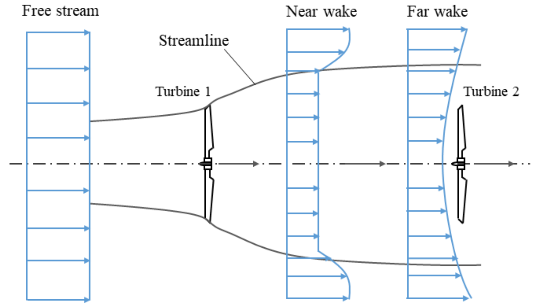
Figure 1 shows an example of the wake effect [21]. The maximum wind energy can be extracted from wind Turbine 1 when a uniform wind passes. However, the passing wind is affected by turbulence, and the wind speed is slowed down by the rotational motion of the blade. This influence has a significant effect on the power output of the turbine located within the wake effect area. In addition, the fatigue loads, such as the motion loading patterns of wind turbines, may increase, and mechanical defects may occur due to the wake effect. As a result, the lifespan of individual turbines can considerably vary, and the operating and maintenance costs of some turbines can be increased. In this study, the main wind direction was analyzed using wind data measurements from an actual wind farm. In addition, the influence of individual wind turbines was verified through a wake model.

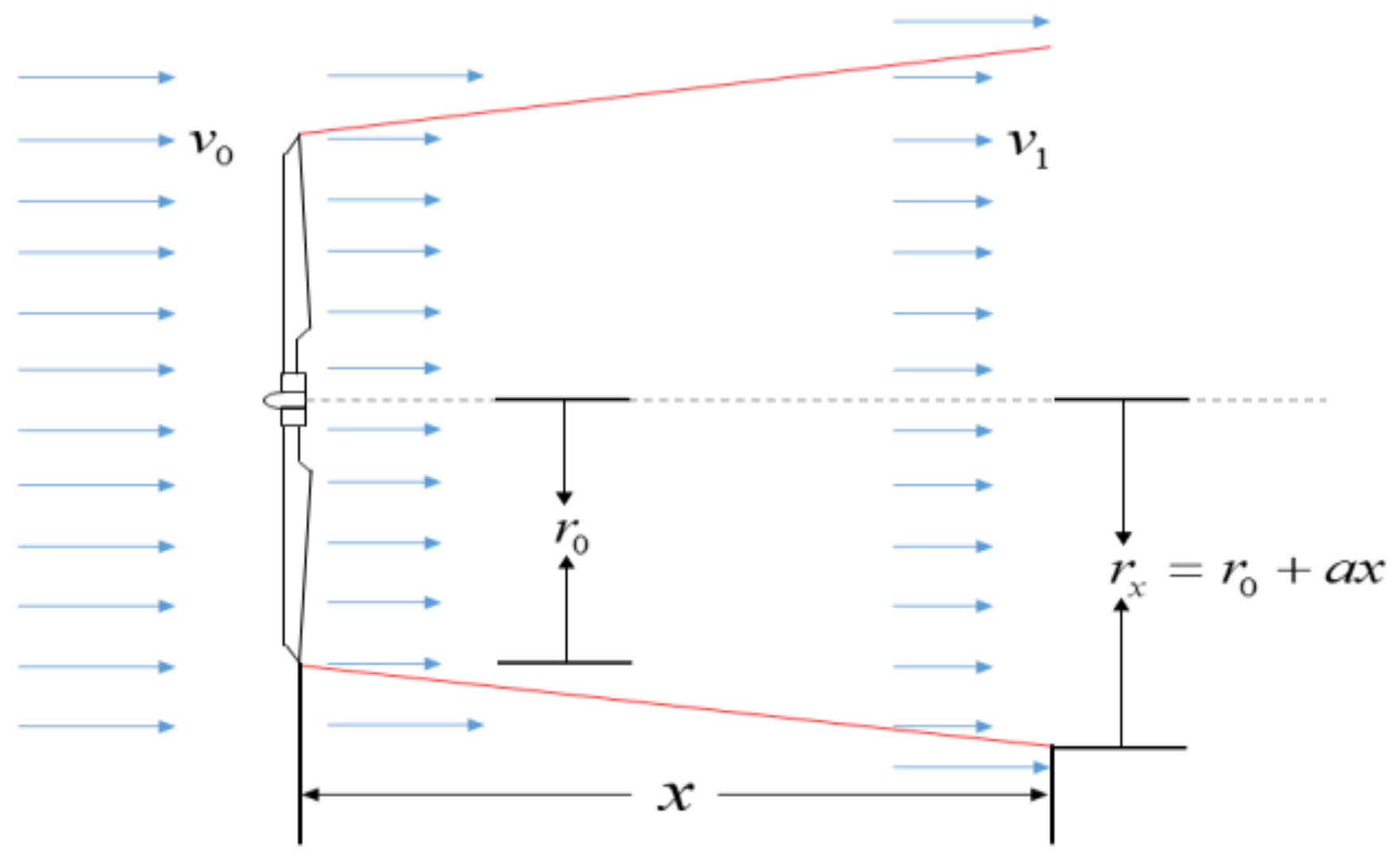
The wind farm’s output tends to decrease due to the wake effect. Minimizing the wake effect when constructing a wind farm layout is necessary. When building the wind farm layout, it should be batched to consider the separation distance of each wind turbine. In this study, active power was decided using the N.O Jensen model, and a long-distance wake model was illustrated, as shown in Figure 2.

According to the Jensen model, the wind speed $v_1$ due to the wake effect is obtained as follows:

$$v_1=v_0+v_0\left(\sqrt{1-C_t}-1\right){\left(\frac{r_0}{r}\right)}^2$$

(1)

where $v_0$ represents the initial wind speed blowing to the blade, $r_0$ is the blade radius, $C_t$ is the thrust coefficient of the turbine, and $r_x$ shows the linear dimension of the diffused wind that underwent the wake effect.

2.2. Active Power Control

In the case of wind power generation, the output is changed according to the wind speed. In particular, the output is changed according to the rotational speed of a wind turbine even when the same wind speed is input. In this process, MPPT controls the speed of the wind turbine to obtain maximum performance and improve the efficiency of power generation. As a result, maximum energy can be achieved under the same conditions. Therefore, wind farms should operate by applying MPPT. However, due to the increase in the grid connection of wind turbines, a grid can reach its acceptance limit. In particular, a wind power generator can increase power generation at night, but the power demand is less at night than at daytime. This means that oversupply is highly likely to occur, and the resulting overvoltage or reverse current may be intensified. Therefore, it is important to have stable operation systems for power supply systems and operate by the control command of the system operator. However, if the output control of wind power generation is not considered according to a grid system’s conditions, the share of wind power generation is limited to a certain level. Thus, large-scale wind farms must have an output control function based on supervisory control. In this paper, we propose the use of an optimal curtailment strategy based on the active power loss when switching from the wind power generator MPPT mode to the output limit control mode.

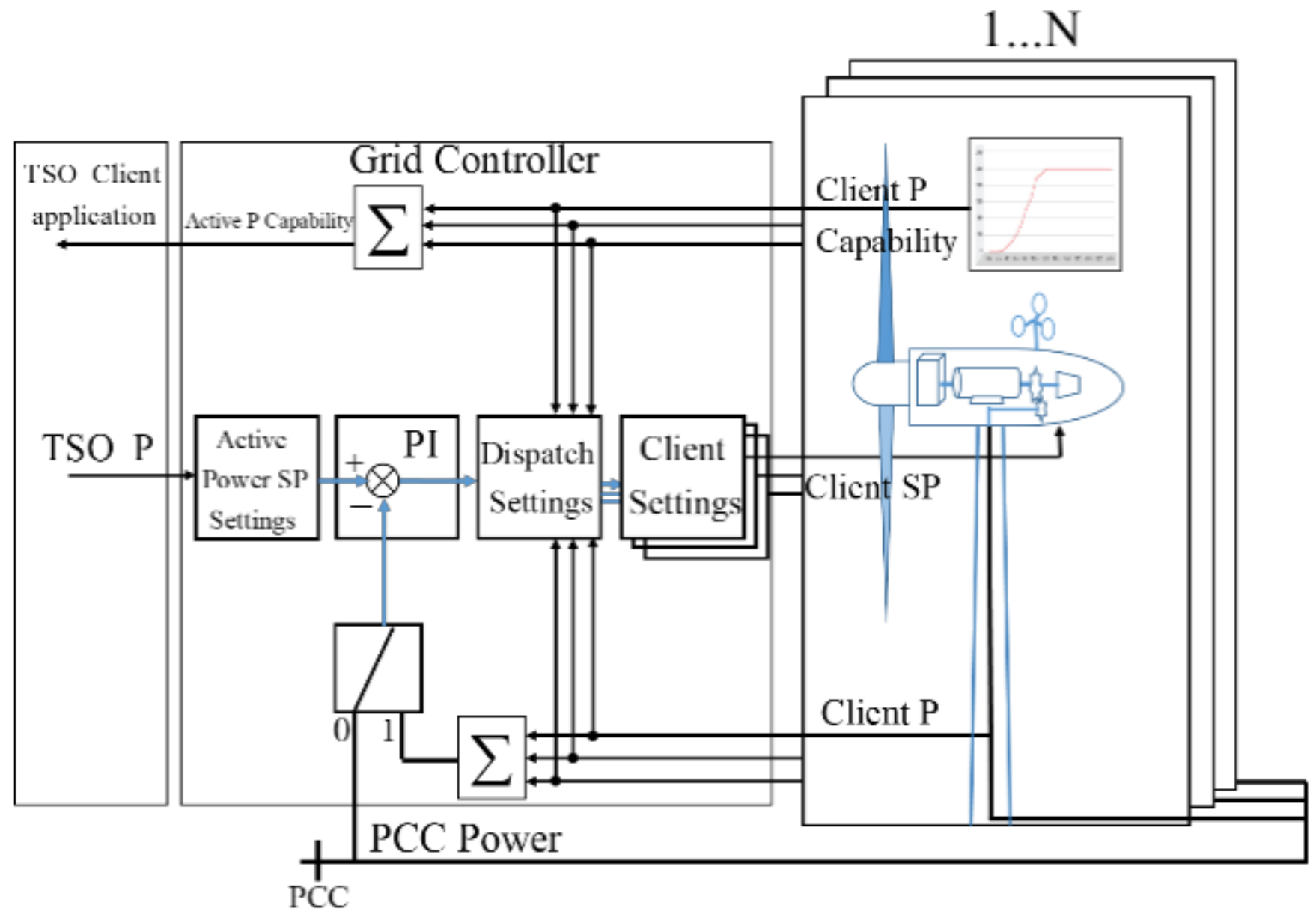
The active power setting SP generally determines the final active power output command based on the following factors: the system operator output command, wind farm operator setting, grid connected operating conditions, and wind farm grid connected standards. The PI controller feeds back the actual active power output using a point of common coupling (PCC) bus. At this time, if there are output fluctuations due to wind farm losses or wind speed changes, the wind farm’s output command is corrected. The active power command of each turbine is derived by reflecting the output measurement value of the PCC using the corresponding logic. In this process, the active power output value of the wind farm, which is required by the transmission system operator (TSO), can be distributed to individual turbines. A schematic diagram of the active power output control of individual wind turbines is shown in Figure 3.

The active power amount of a wind power farm is expressed as follows:

$$P_{WF}={\displaystyle \sum }_{k=1}^N{P}_{W{T}_k}+P_{loss}$$

(2)

where $P_{WF}$ is the total power of the wind farm measured at the PCC point, $P_{W{T}_k}$ is the power generated by an individual wind turbine, and $P_{loss}$ is the output power loss.

In general, wind turbines reduce output power to a certain part from a generator’s maximum capacity to balance supply and demand. In addition, wind turbines stably maintain frequency through output control in response to sudden load increases [22]. The wind farm curtailment command based on the weight assigned to each turbine is as follows:

$$cu{r}_{WF}={\displaystyle \sum }_{k=1}^N{w}_{k}cu{r}_{W{T}_k}$$

(3)

At this time, the individual weights of $w_k$ are based on the sum of the total 1 and are expressed as follows:

$${\displaystyle \sum }_{k=1}^N{w}_k=1$$

(4)

where $k^{ }$ is the number of wind turbines in a wind farm, $cu{r}_{WF}$ is the power limit of the wind farm, $w_k$ is the curtailment weight allocated to individual wind turbines, and $cu{r}_{W{T}_k}$ is the curtailment of individual wind turbines.

This paper proposes a method to effectively reduce losses by focusing on the power losses caused by curtailments. The proposed method is expected to reduce the curtailment imbalance and the unilateral burden on wind power operators.

3. Monte Carlo-Based Weighting

3.1. Loss-Based Objective Functions and Constraints

The active power of a wind farm is controlled by a certain ratio of the output power through proportional distribution (PD) control. This method is simple and has a low computational load. However, it is considered inappropriate for minimizing the losses occurring in the process of allocating active power. Therefore, in this paper, a loss function is presented. Moreover, the optimal command value of individual wind power generators was calculated and then distributed to individual turbines based on the loss function. The objective functions based on the load data of each section line from an array to the wind turbine and the PCC is the same as in Equation (5). In accordance with the curtailment reference, the output power value for each turbine was calculated while focusing on loss reduction based on the proposed loss function.

$$Mi{n}^{ }{\displaystyle \sum }_{n=1}^N{r}_{n·n-1}·\frac{P_{ref·n}{}^2+Q_{ref·n}{}^2}{V_{n,n-1}{}^2}$$

(5)

where $P_n$ and $Q_n$ represent the active and reactive power command values of the wind turbine, $V_n$ is the voltage fluctuation in the $n_{ }$ bus, and $r_n$ is the resistance load in the n bus.

The objective function derived for calculating the weight based on a random number is expressed as follow:

$$\begin{gathered} X_n=Ran\left(i\right)\times \frac{1}{\delta }+\frac{1}{\delta } \\ {X}_n=X_{n-1}+Ran\left(i\right)\times \frac{1}{\delta }+\frac{1}{\delta } \end{gathered}$$

(6)

where $i_{ }$ represents a range of random numbers greater than 0 and less than 1, and $\mathsf{\delta }$ is a standard deviation for setting random numbers.

Based on Equation (6), the reduction weight assigned to each turbine was derived as shown in Equation (7). The corresponding weight was derived using the generated random number and total output limit command.

$$w_n=X_{n-1}+\left(cu{r}_{WF}-{\displaystyle \sum }_{n=1}^N{X}_n\right)/N$$

(7)

where $X$ is a random number for representing the weight, and $cu{r}_{WF}$ is the total wind farm output.

According to the curtailment reference, the power value of individual turbines was calculated and prepared as a look-up table based on the proposed loss function.

3.2. Monte Carlo Simulation

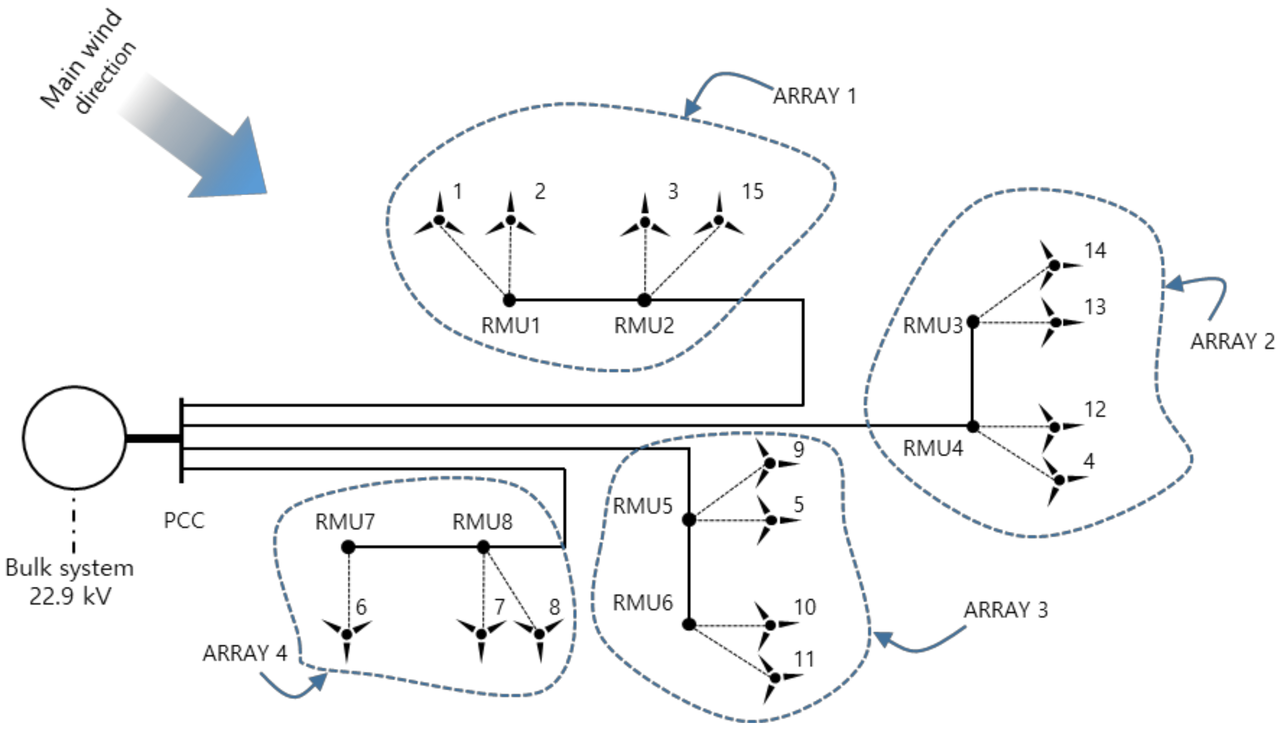
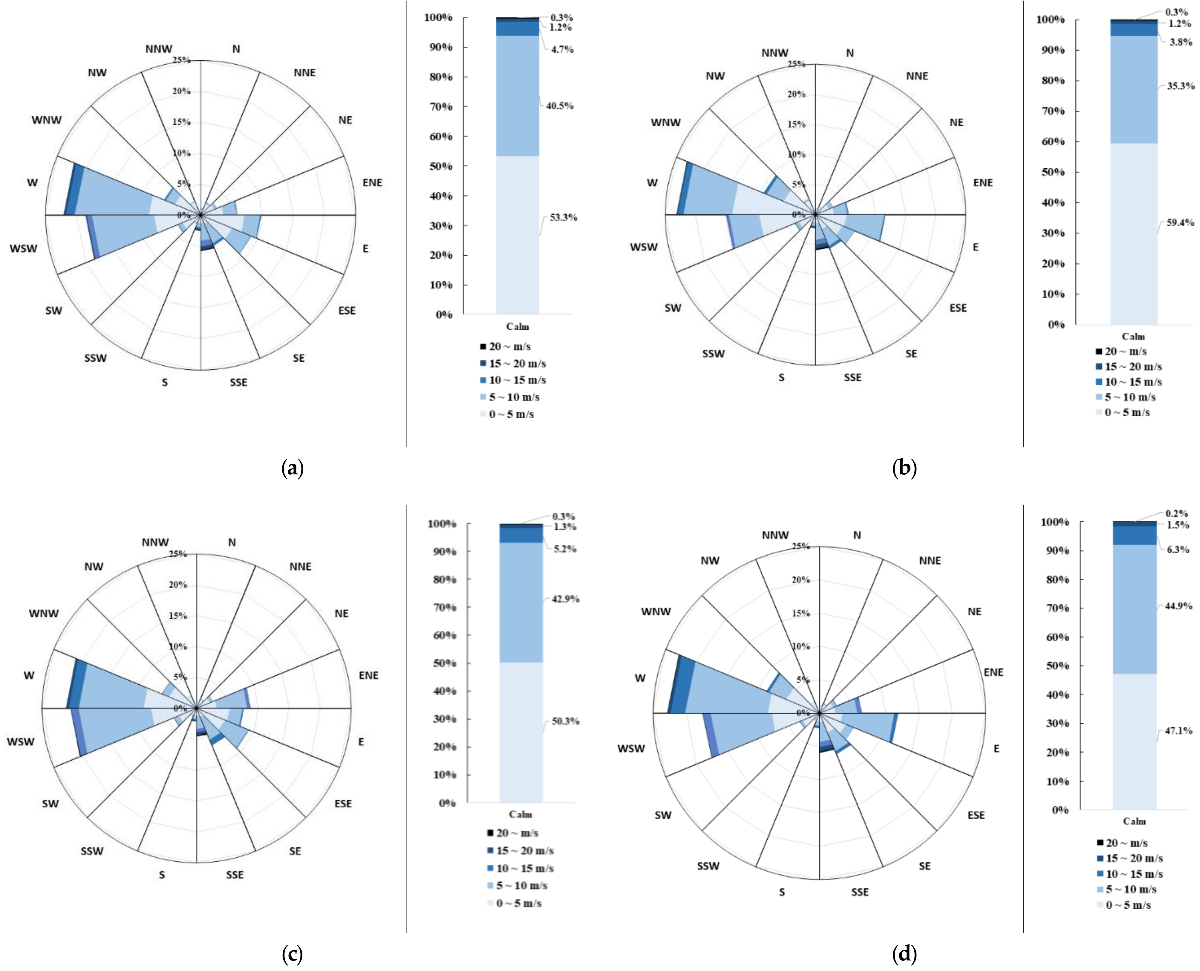
Monte Carlo is a wide range of algorithmic techniques that repeatedly use random sampling methods to achieve mathematical results and determine probability distributions for uncertain input variables. Furthermore, the results are derived according to a simulation repetition established by a random sample. This method is applied in optimization, numerical integration, and derivation from percentage distribution. In this work, the optimal value of active power was distributed to individual turbines using the Monte Carlo method while considering various weather conditions. The main wind direction of the wind farm was set based on measured wind data considering the wake effect according to the layout of the wind turbine. 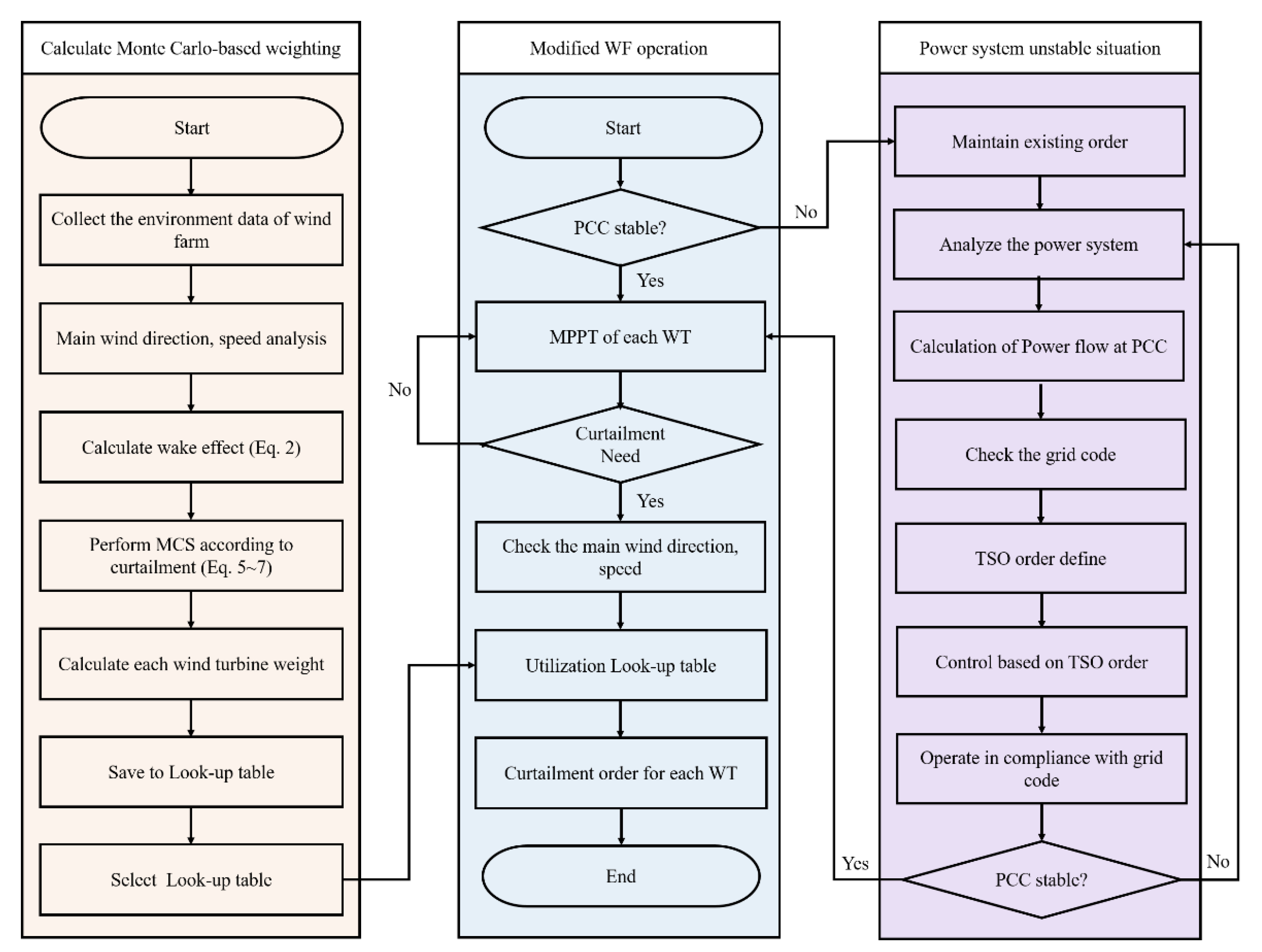Figure 4 shows the algorithm performed by applying the Monte Carlo simulation. The active power command values were suitably distributed for individual wind power generators according to the algorithm.

The proposed algorithm differently distributes the values of individual turbines when it distributes the total active power command of a wind farm to individual turbines. First, the wind direction and speed data are collected from the environmental data of wind farms. The wind speed distribution along the main direction is analyzed through the collected data. Then, each output quantity is calculated considering the wake effect of each wind power generator on the analyzed wind condition data. Assuming that the output limit signal is input to the calculated wind power generator, the weight of the curtailment from each wind power generator was obtained using the proposed loss reduction objective function. The individual output data of the wind power generator according to the output limit was converted into a look-up table. When an output limit command is input, the active power output limit command is distributed by selecting it according to the order. Wind farm curtailment is performed using the look-up table. Before the curtailment order, the wind farm performs the MPPT operation. The system operator decides whether to curtail power or not based on the power supply and system demand and sets a command. Then, the optimal individual turbine command value from the look-up table is selected and distributed based on the current status of the wind farm and the set curtailment command information. However, the system operator the unstable state of the grid must be considered. Control that complies with the grid code should be prioritized for the power system’s stable operation. Determine the stability of the PCC and, in the case of unstable situations, operate according to the power system unstable situation algorithm. According to the existing command, the power system is analyzed. The power flow of PCC is calculated based on the analyzed power system result. A new TSO command is established based on the grid code and the analyzed power system state. The established TSO command is controlled for the stabilization of the power system. When the system is stabilized, control is performed according to the order of the modified WF operation algorithm.

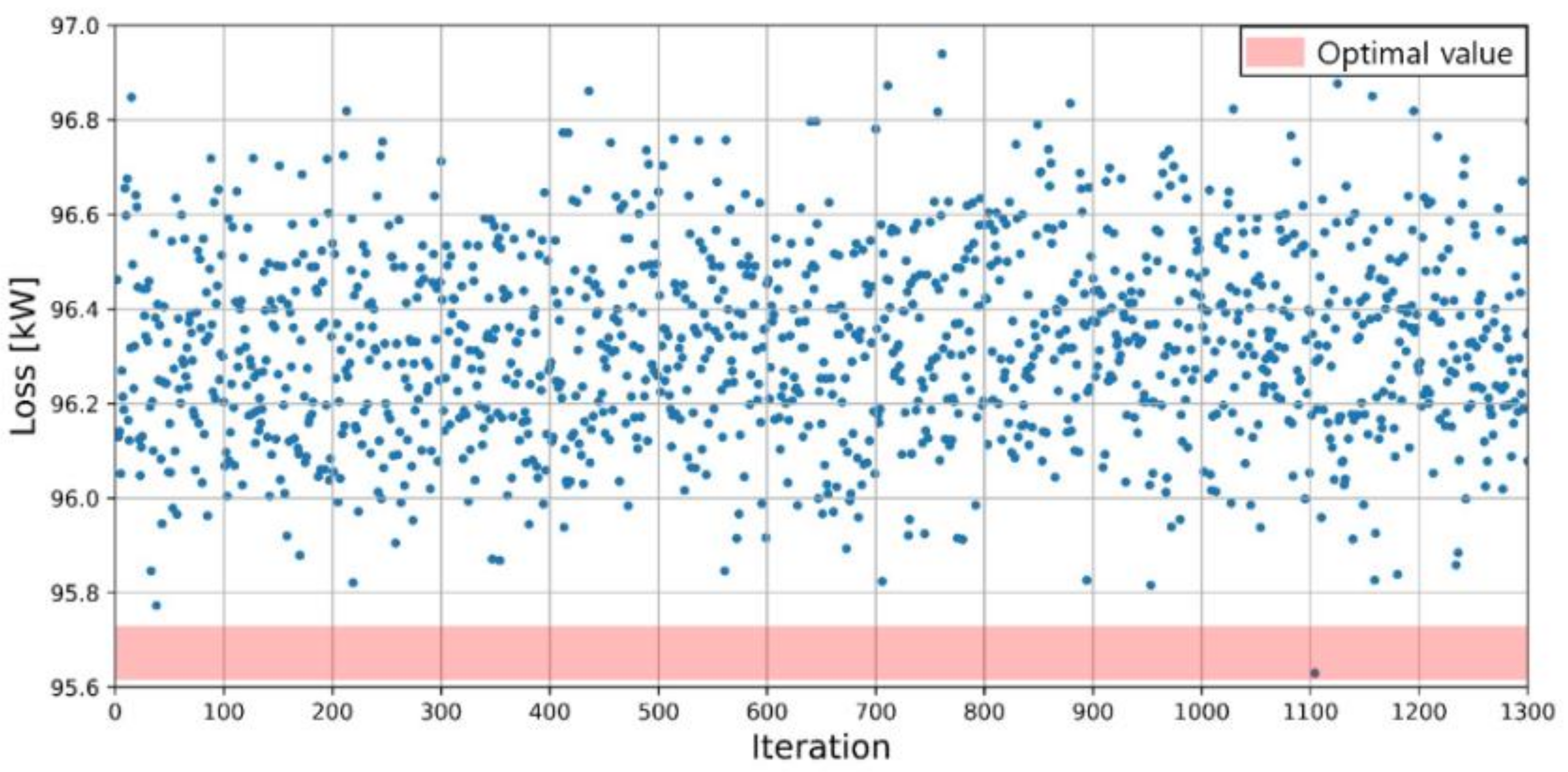
Monte Carlo simulations were performed to find optimal command values by generating random numbers based on loss reduction. The x-axis is the number of iterations based on the active power distribution value. For each iteration, different weights were derived based on random numbers, and the active power values were applied to individual turbines using the weights. According to each assigned active power value, the y-axis is the power loss value at the PCC point. Typically, Monte Carlo simulations are performed on a 10,000 basis. In this paper, as a result of running 10,000 simulations, no advanced results were obtained even when more iterations of 1300 times or more were performed. Therefore, the results of up to 1300 times were derived as a graph, as shown in Figure 5.

3.3. HILs (Hardware-in-the-Loop Simulation)

HILs is a technology used for developing and testing complex embedded systems in real time. The HILs components include simulators that mathematically model systems and environments in which HILs target devices are operated. The simulator performs the function of simulating the operating environment of the HILs target devices in real time and uses HILs to build a simulated environment close to an actual operating environment to test the HILs target devices. To develop an embedded system with great precision, it is necessary to perform experiments on the entire system to which the system belongs in a real environment. However, it is practically impossible to perform tests in a natural environment. In particular, when the target system is a wind farm, this task becomes impossible due to economic viability and accessibility. Therefore, HILs is an effective method when conducting wind farm-based research because it provides test environments similar to actual environments. In addition to these advantages, HILs can significantly reduce the development time and cost by detecting errors, taking actions to fix them, and performing trial and error in advance.

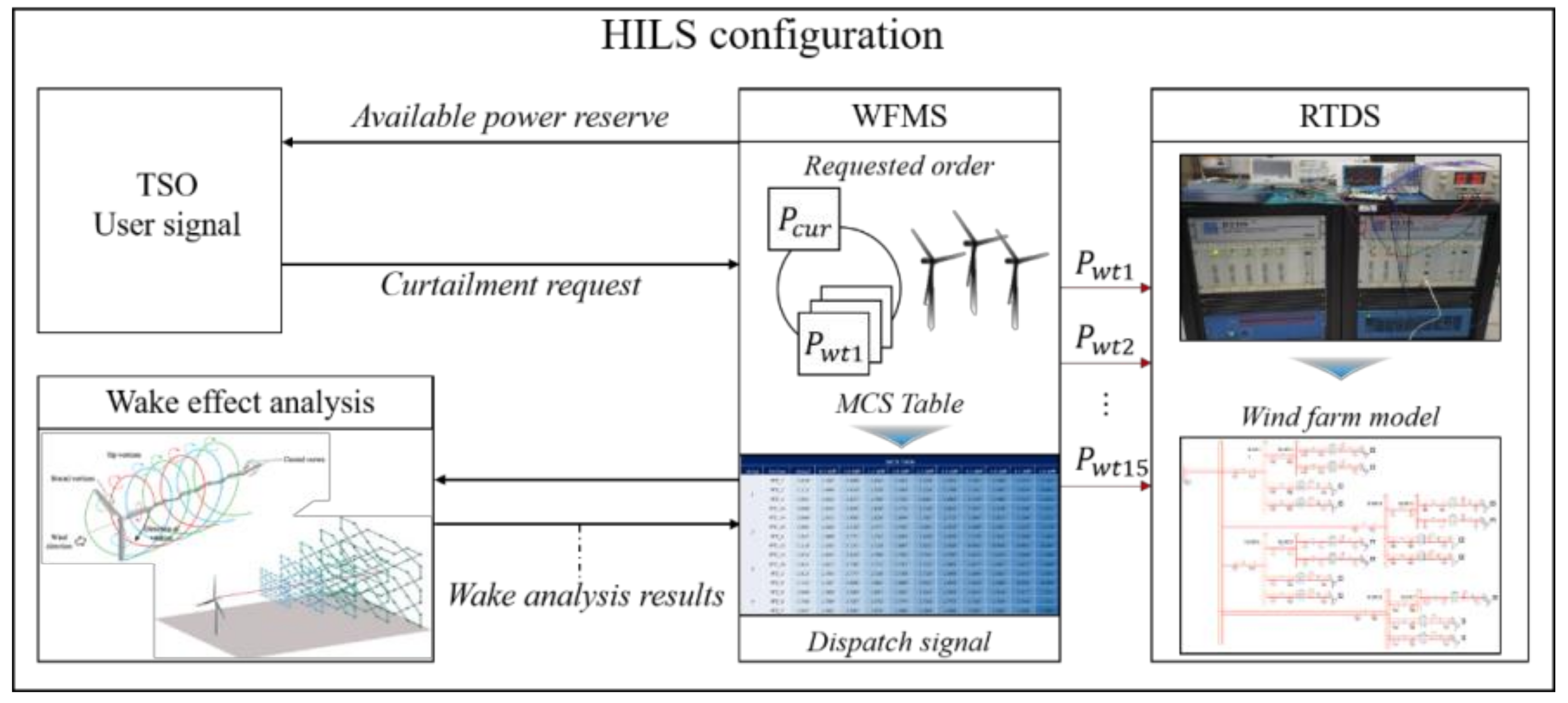
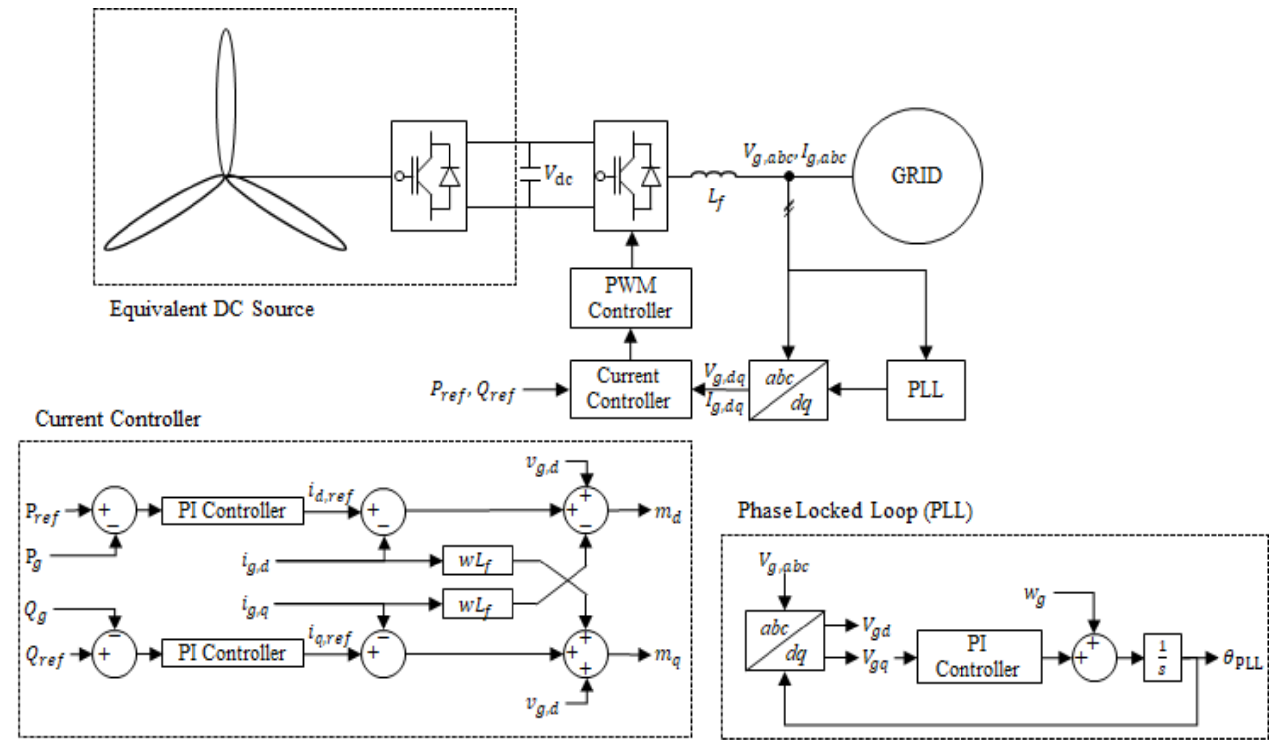
Figure 6 shows the HILs configuration for active power control in a wind farm. The TSO controls the stable power supply based on the wind farm data obtained through the wind farm management system (WFMS). When the wind farm produces more energy than required by the TSO, an output limiting signal is transmitted. In the WFMS, the output limit command value required by the TSO is distributed to individual wind turbines. At this time, the command value is calculated considering the wind turbine wake effect and the loss-based Monte Carlo method. In addition, the signal of the distributed command is entered in the HILs configuration to perform control. In this paper, each wind turbine in the wind farm was assumed as a full converter interfaced model. A simplified wind turbine model implemented in HILs configuration is depicted in Figure 7 as the control strategy proposed in this paper is focused on the grid side converter to minimize active power loss within the wind farm by controlling the active power of each wind turbine. The active and reactive power injected from each wind turbine can be computed as Equations (8) and (9).

$$P_g=\frac{3}{2}\left(v_{gd}{i}_{gd}+v_{gq}{i}_{gq}\right)$$

(8)

$$Q_g=\frac{3}{2}\left(v_{gq}{i}_{gd}-v_{gd}{i}_{gq}\right)$$

(9)

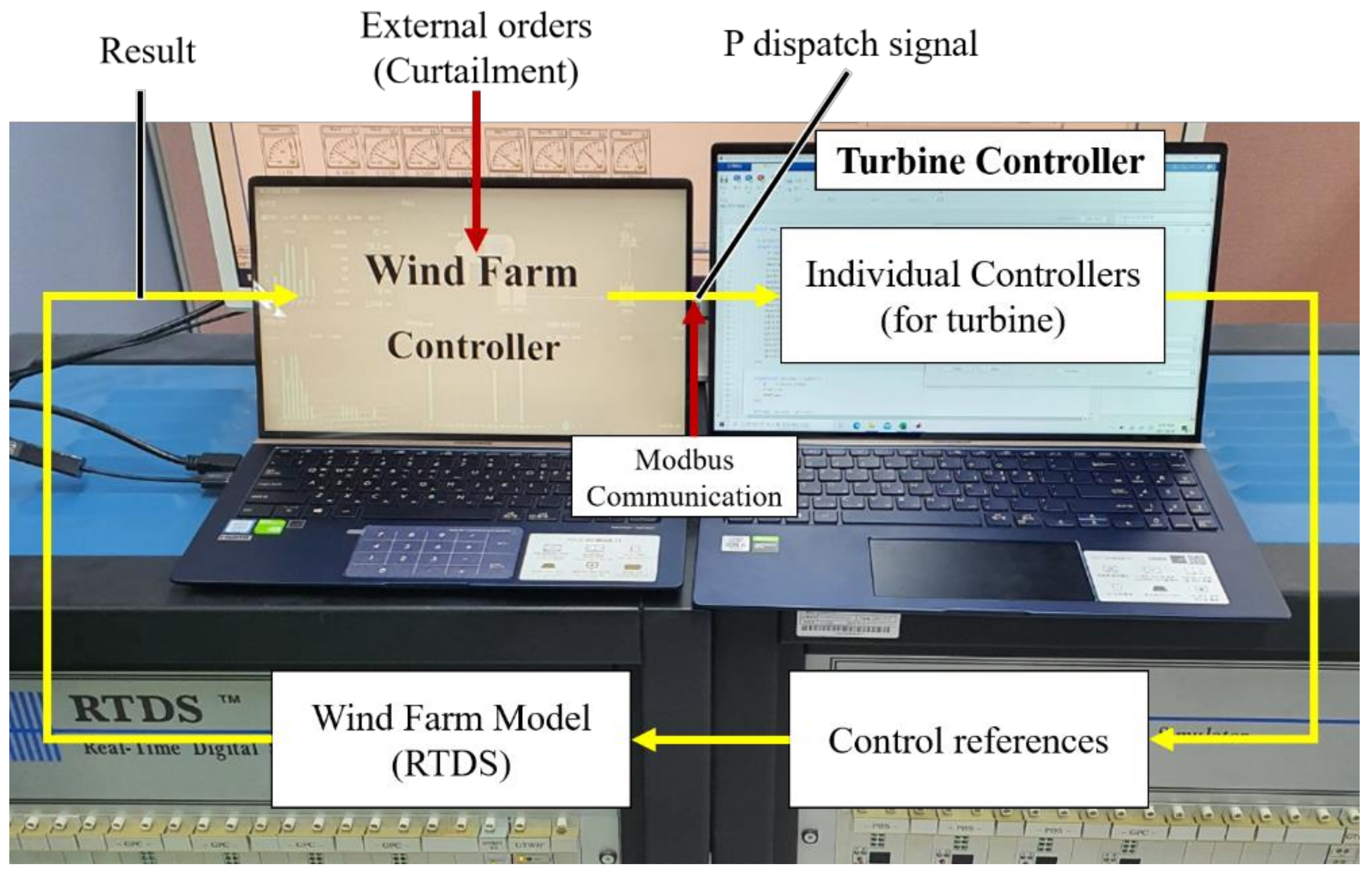
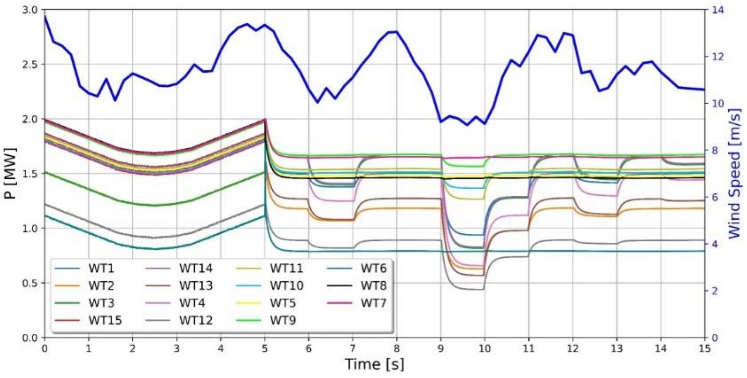
The control structure flow, including the implemented real HILs, is shown in Figure 8. The HILs consist of a separate computer as a wind farm controller, a turbine controller, and a grid model of the RTDS. Each PC was configured by reflecting individual algorithms according to their roles. When an active/reactive signal is received, the wind farm controller sends the control signal to each turbine, and the RTDS operates based on the control signal. It is a structure in which the PC manages the signal, and the signal is transmitted using the MODBUS protocol. When surplus power is measured, the wind farm controller may receive the TSO curtailment signal. The transmitted signal outputs the curtailment signal of the individual wind turbine according to the control command established in the MCS table from the wind farm controller. The curtailment signal is entered as a dispatch signal to the wind farm configured in RSCAD based on the equivalent model expressed in Figure 7. Through the curtailment signal, the individual wind turbines and the PCC’s changed output are monitored in real time by the wind farm controller. A mode bus protocol was used to send and receive control signals during this process. In addition, the amount of power loss reduction of the proposed method can be confirmed through this control structure.

4. Discussion

4.1. Simulation Model Configuration

In this paper, Jeju Island, which has a large proportion of annual average curtailments due to increased wind generation, was selected as a target area. Figure 9 shows the structure of the Jeju Dongbok Wind Farm. Figure 10 describes the wind-rose which was obtained by measuring the wind flowing into the wind turbine of Array 1 of the Dongbok wind farm from 1 May 2019 to 30 May 2019. This pattern was analyzed based on the main factors: wind direction, frequency, and speed. In addition, the wind-rose in this paper was based on the Weibull distribution function and the Von Mises distribution function. For the Weibull distribution function ranking coefficient, the wind speed with the highest probability of occurrence was designated, and other wind speeds were derived as shape coefficients as a function of value. In addition, the wind direction distribution map was derived based on the Von Mises distribution function, and the average of the wind direction data was applied as the function parameter. In this study, the main wind direction was set through the presented wind direction and speed data. The wind direction was determined by north (N), south (S), east (E), west (W), and azimuth (0–360°). Furthermore, all the information displayed in the data set applied 16 azimuths as the default direction. It was possible to confirm the main wind direction of the wind farm and the proportion of the wind speed for each wind direction through wind data. The main wind direction was in the W direction, and it was confirmed to be 292.5° at 270°.

Table 2. Wind speed data measured at the main wind direction (west 270°).

Group	Wind Speed
Array 1	WT1	WT2	WT3	WT15
	11.54 m/s	10.02 m/s	12.64 m/s	13.16 m/s
Array 2	WT14	WT13	WT4	WT12
	13.08 m/s	10.34 m/s	11.19 m/s	9.40 m/s
Array 3	WT11	WT10	WT5	WT9
	11.86 m/s	11.59 m/s	11.07 m/s	8.95 m/s
Array 4	WT6	WT8	WT7
	13.74 m/s	10.99 m/s	12.78 m/s

shows the data based on the wind flowing from the main wind direction (W direction) of the Dongbok wind farm.

The wind turbines (WT1, WT3, WT15, WT14 WT11, WT6, and WT7) face wind in front of the leading wind direction. Since the turbine’s wind speed is not affected by any obstacles, the wind turbines mentioned above were set to free wind. The wind turbine considered in this study had a rated wind speed of 12 m/s. According to Figure 9, the actual wind speed data comprised the main wind direction (W 270°) and the wind speed of the wind turbines at the front (11.5 m/s or more). However, in the case of the wind turbine located at the rear, the wind speed was found to be lower than that of the wind turbine at the front (11.5 m/s or less). The minimum wind speed was measured by the wind turbine (WT9), and it was found to be 8.95 m/s. In particular, WT2, WT4, and WT13, which are located at the rear end of WT1, showed wind speed decreases compared with the initial wind speed. This was because the rear-installed wind turbines faced low wind speed caused by the rotational movement of the front wind turbine rotor blades. Furthermore, the wind speed attenuation due to the wake effect depended on the distance between the wind turbines.

To apply the proposed method, a simulation was constructed using the RSCAD tool. The selected wind farm consists of 15 Hanjin 2 MW doubly fed induction generator (DFIG) wind generators. The wind farm consists of one array of three or four wind turbines. In the case of grid-connected structure, the wind farm consisted of a voltage of 22.9 kV, also connected to the system by boost from central substation facilities. The initial MW output was set by inputting the wind speed data measured in the main wind direction of the configured wind farm. In the simulation scenario, the power losses according to the curtailment signal were derived and compared.

4.2. Simulation Results

The PCC power value was measured by inputting the command value to the wind farm based on the configured RSCAD. The simulations were conducted for 15 s, including 5 s for initial stabilization. After the initial stabilization step, the set command value was input according to the curtailment signal.

Table 3. Maximum output setting value according to the curtailment signal.

Array	Turbine	Control
		PD		MCS Table
		Ratio	PMax [MW]	Ratio	PMax [MW]
1	WT1	0.067	1.497	0.1365	1.147
	WT2	0.067	1.182	0.1067	0.981
	WT3	0.067	1.648	0.126	1.351
	WT15	0.067	1.667	0.1158	1.421
2	WT14	0.067	1.667	0.0958	1.521
	WT13	0.067	1.272	0.087	1.170
	WT4	0.067	1.514	0.0764	1.465
	WT12	0.067	0.885	0.0662	0.887
3	WT11	0.067	1.542	0.0574	1.588
	WT10	0.067	1.508	0.0464	1.609
	WT5	0.067	1.480	0.0356	1.635
	WT9	0.067	0.789	0.0246	0.999
4	WT6	0.067	1.667	0.0156	1.922
	WT8	0.067	1.463	0.009	1.751
	WT7	0.067	1.654	0.001	1.982

shows the maximum command set values and the allocation ratio according to the curtailment signal of 5 MW. The curtailment signal written in the table was an input signal calculated by the PD control method and the proposed method (MCS). In the case of the PD control method, the 5 MW curtailment signal was distributed at a constant rate to 15 wind turbines. The PD method of the generic output control applied the same allocation ratio of 0.067 and controlled each wind turbine in a curtailment amount of approximately 0.33 MW. Furthermore, the proposed method controlled the power values of individual wind turbines according to each other allocation ratio in the look-up table.

Figure 11 and Figure 12 show the actual active power of the wind farm based on two methods (PD, MCS Table) when inputting a curtailment signal of 5 MW. They also show the wind speed data continuously blowing into the wind farm. The curtailment signal was entered at 5 s when the wind turbine MPPT control was in progress. Both methods distributed the curtailment allocation ratio of the individual turbines, and the active power output could confirm that limit.

Figure 13 shows the PCC bus voltage comparison according to the output limit of the two methods. In both methods a voltage drop occurred from the curtailment signal. The voltage drop could be observed due to the decrease in the power factor, since a proportional relationship between the active power and power factor was established. Additionally, the voltage fluctuation at the curtailment time was 0.95–1.05 p.u., showing a stable status.

Figure 14 shows the power graph of the PCC bus based on the two control methods (PD, MCS Table) when inputting an output power limit command of 5 MW. The loss reduction effect of the proposed method was confirmed through the main analysis for 6–13 s when the output limit was applied. As shown in the enlarged graph, the loss reduction effect of the proposed method was verified in the loss reduction section. Furthermore, it can be seen that the loss reduction effect increased when the output quantity of the whole wind turbine decreased.

Table 4. Numerical result for the simulation.

Section	PD			MCS			Improved Quantity [kWh]
	PWF [MW]	PPCC [MW]	Loss [kW]	PWF [MW]	PPCC [MW]	Loss [kW]
Pave	24.4300	20.5343	3895.7	24.4300	20.7054	724.69	0.8808
P1section	20.9847	19.8969	1087.8	20.9847	20.5782	406.50	0.1892
P2section	15.6323	15.2751	357.2	15.6323	15.5976	34.70	0.0895
P3section	19.8491	19.0172	831.9	19.8491	19.6929	156.20	0.1876
P4section	21.4858	20.2982	1187.6	21.4858	20.8684	617.40	0.1583

shows the effect of decreasing the losses based on the two case studies. When instructing a curtailment signal of 5 MW, an average loss of 10 s was measured, from 5 to 15 s in the two case studies. Regarding the average loss measurements, the proposed method showed an improvement of 3.171 MW compared with the measured average loss of the PD method. In addition, regarding the loss improvement analysis, the loss reduction was evaluated by dividing it into four sectors. When the order was expressed as a loss ratio, it was found that the loss reduction in sector 1 had the greatest effect. Considering that this is an instantaneous power indicator, the improvement effect in terms of the power amount is expected to be even more significant. In addition, the loss reduction effect is expected to increase further when applied to large-scale wind farms in the future.

5. Conclusions

In this paper, a study was conducted on optimization command values according to curtailment signals. The proposed method is based on power losses, and the Monte Carlo algorithm was applied to assign curtailment signals. Next, a simulation was performed by making the calculated values in a look-up table based on the proposed algorithm. In the case of a power curtailment requirement from the TSO, the proposed method showed that the computational burden of the wind farm controller could be reduced while reducing the active power loss. As the simulation results show, the power loss could be improved compared with that of the proportion distribution method when controlling the MCS table method to actual wind farms. When applied to a large-scale wind farm, the amount of power loss improvement is expected to increase. Additionally, it is expected that more sophisticated design simulations can be performed through linkage with existing wind farm management systems using the RTDS model. However, there are still some shortcomings that need to be completed. Based on this study, it is necessary to further explore the control for wind directions other than the main wind direction. This helps reduce power loss with the active power control flexible in various output limiting scenarios. In addition, the detailed controller needs to be modified to reflect momentary changes in system conditions such as accidents. Finally, from the operation viewpoint, a detailed economic analysis should be done based on power loss reduction.