
Improved Optimal Control of Transient Power Sharing in Microgrid Using H-Infinity Controller with Artificial Bee Colony Algorithm


Abstract
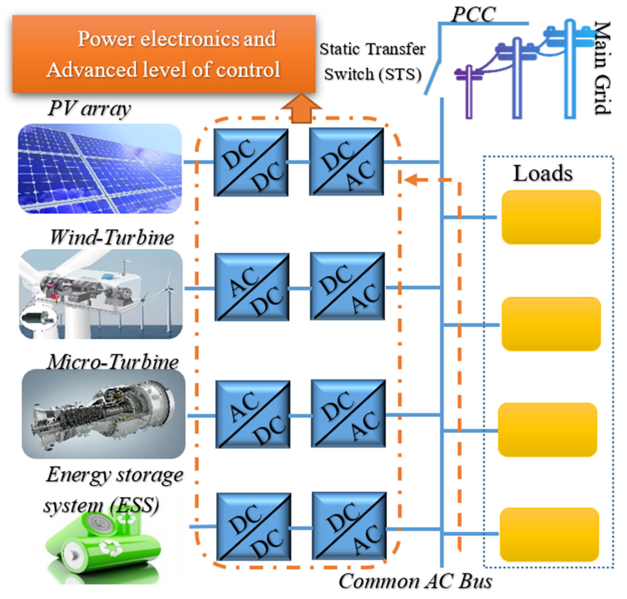
:1. Introduction
2. Mathematical Modeling and Optimization Algorithms
2.1. Particle Swarm Optimization Algorithm
2.2. Artificial Bee Colony Algorithm
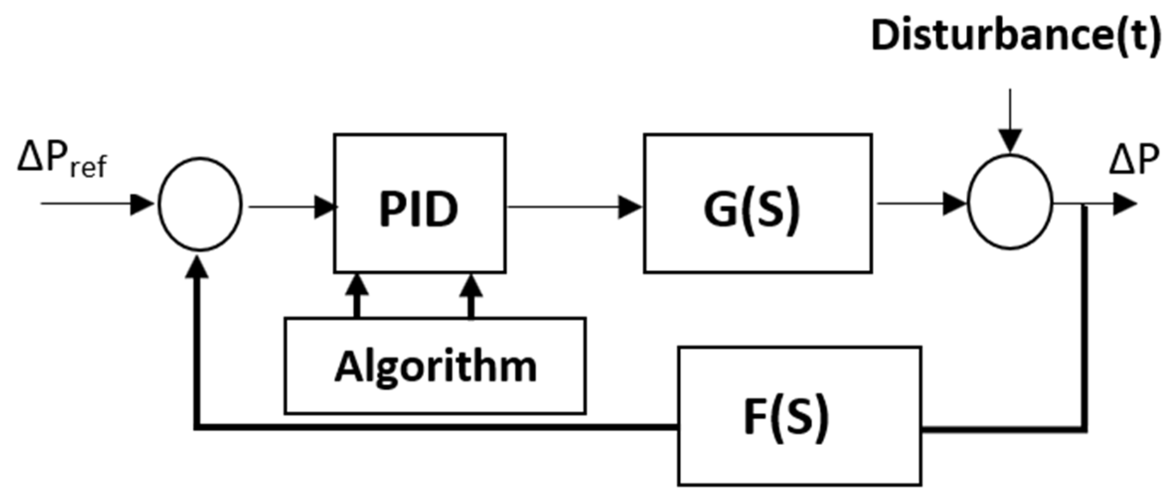
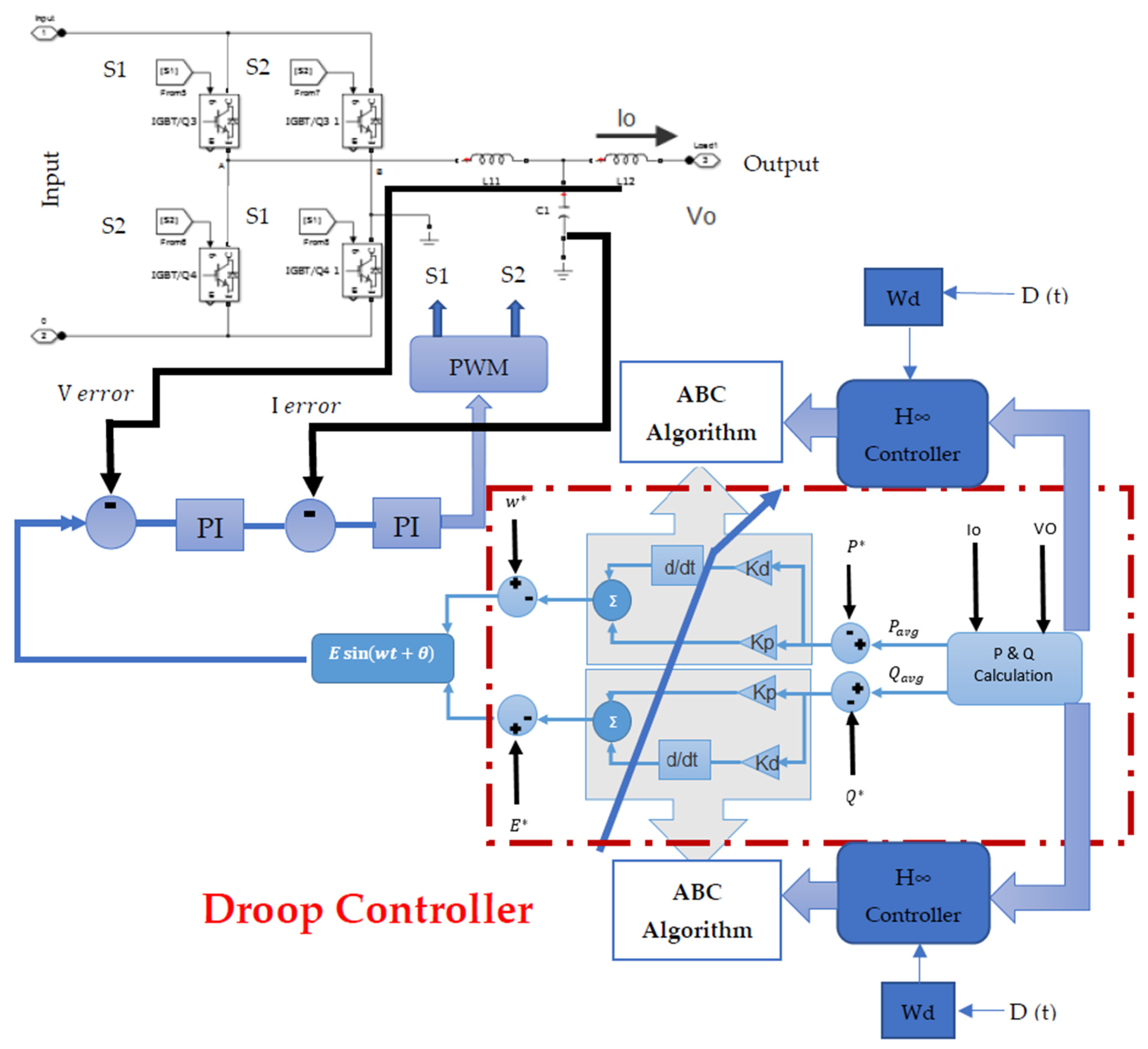
3. Controller Design
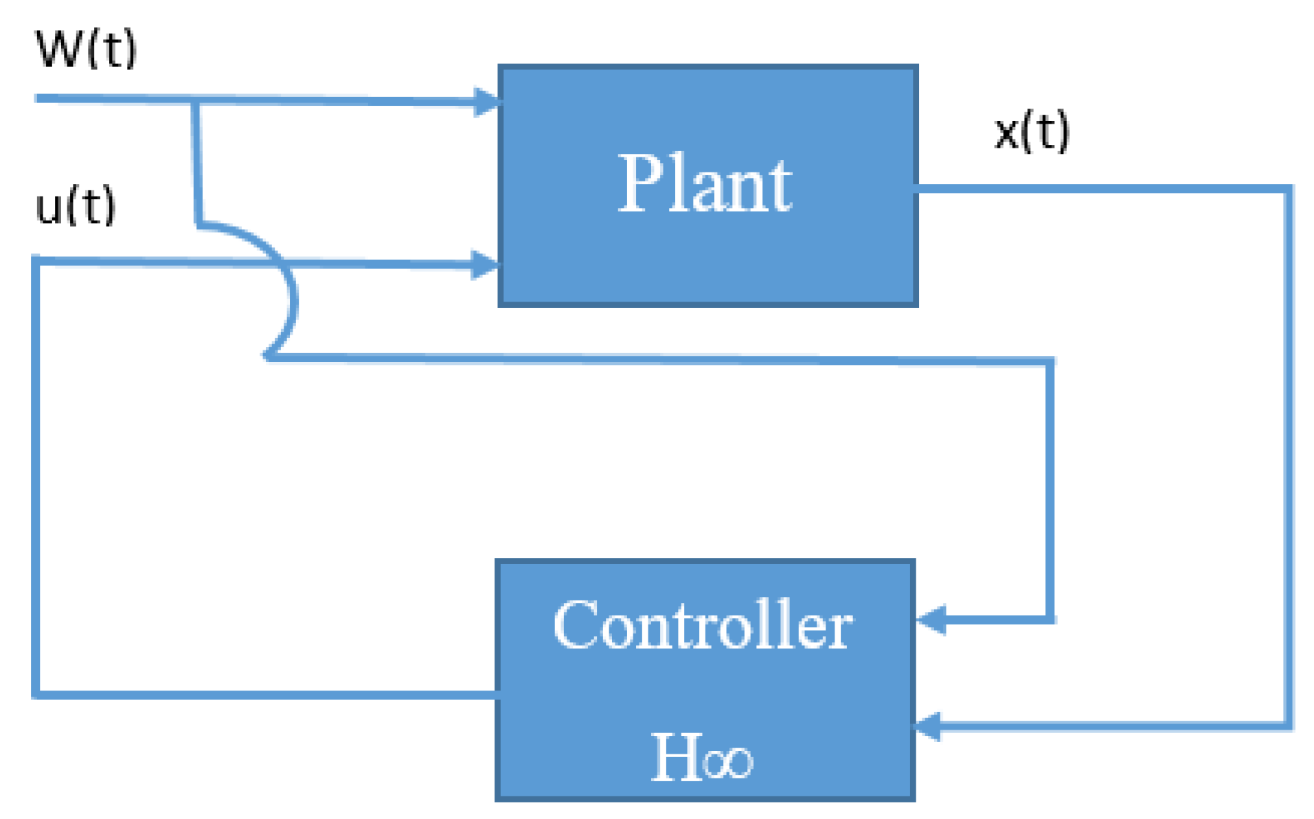
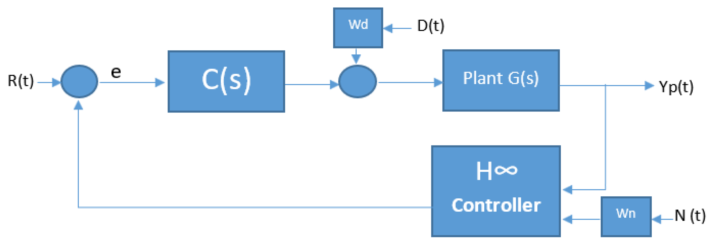
3.1. Design of H∞ Optimal Controller
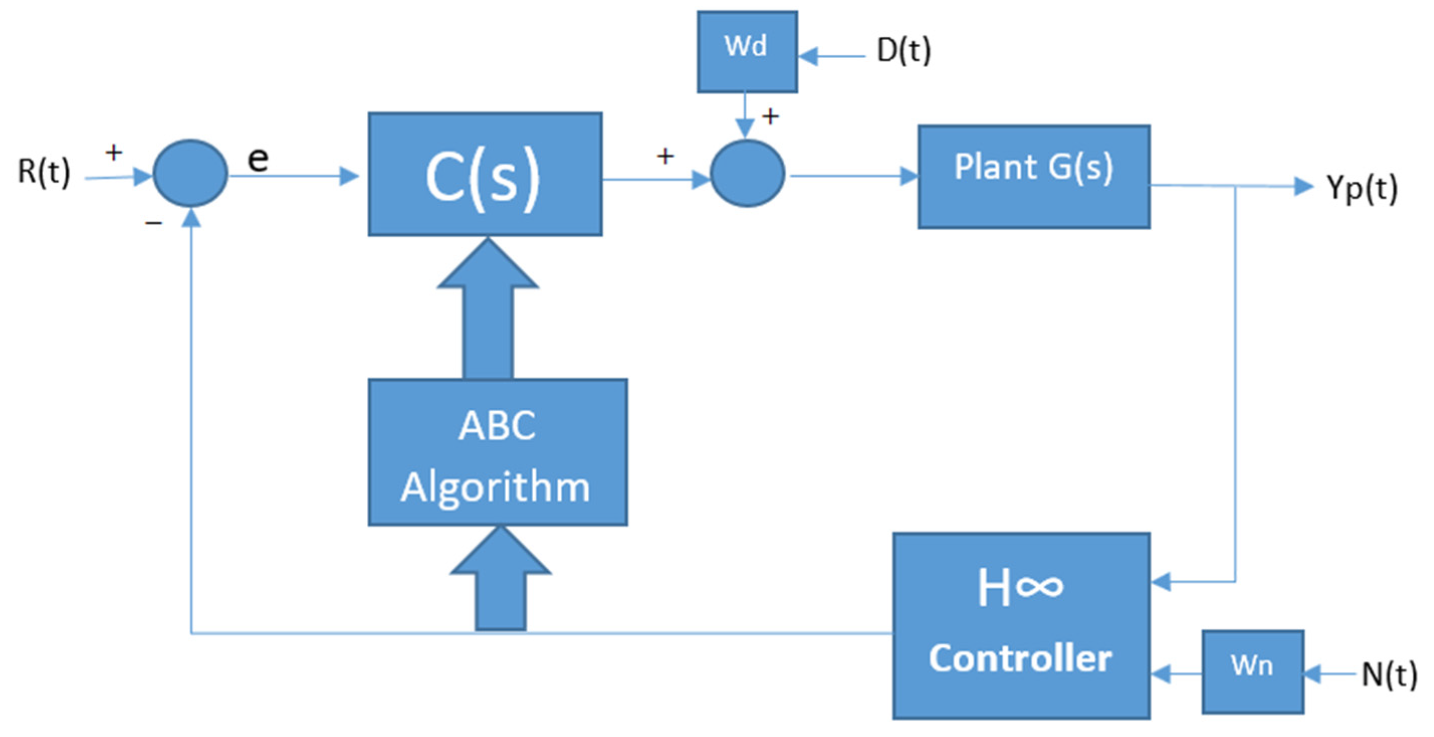
3.2. Design of PID H∞ Optimal Controller with ABC Algorithm
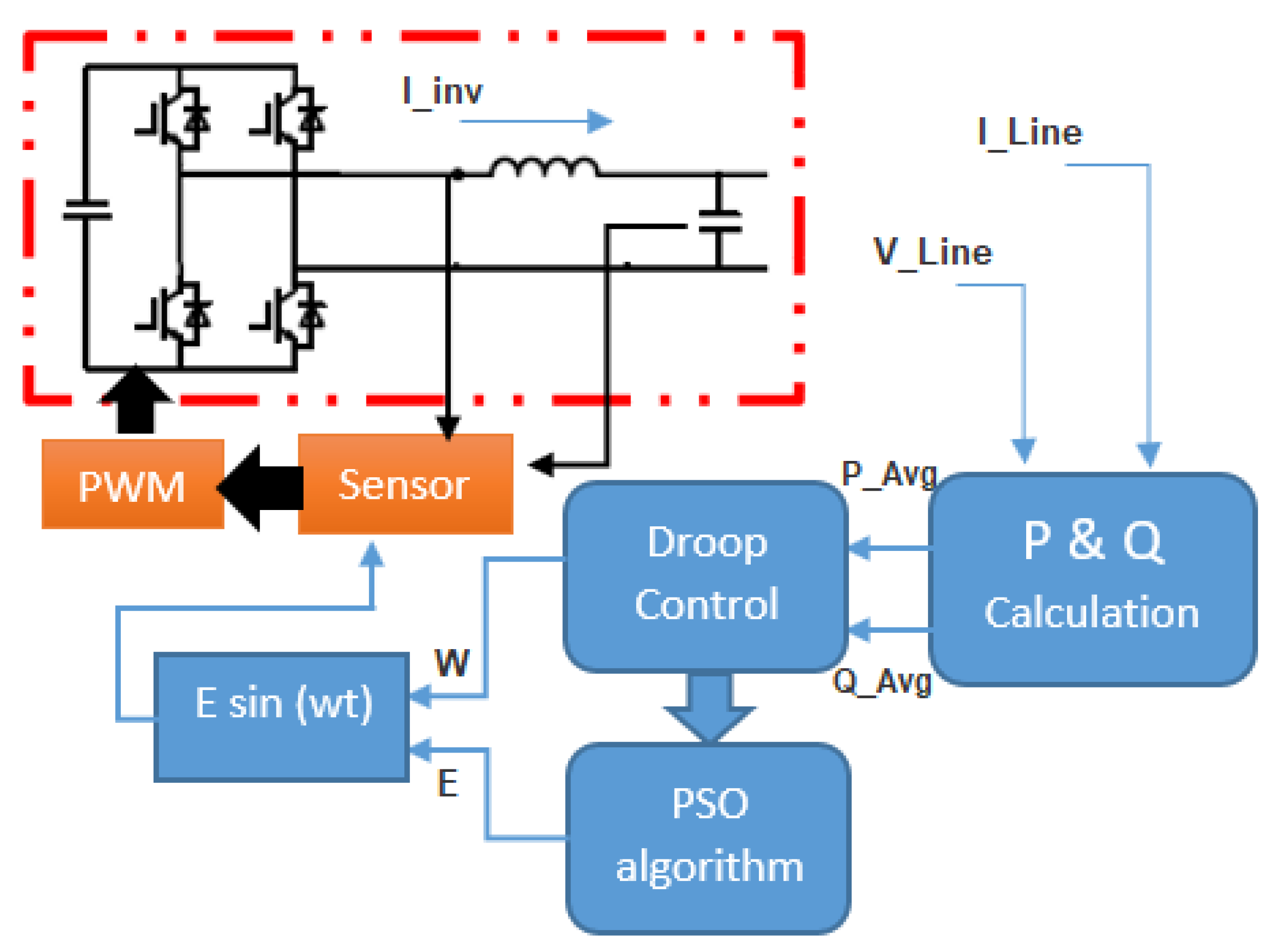
4. Optimized Droop Control Parameters by H∞ Optimal Controller with ABC Algorithm
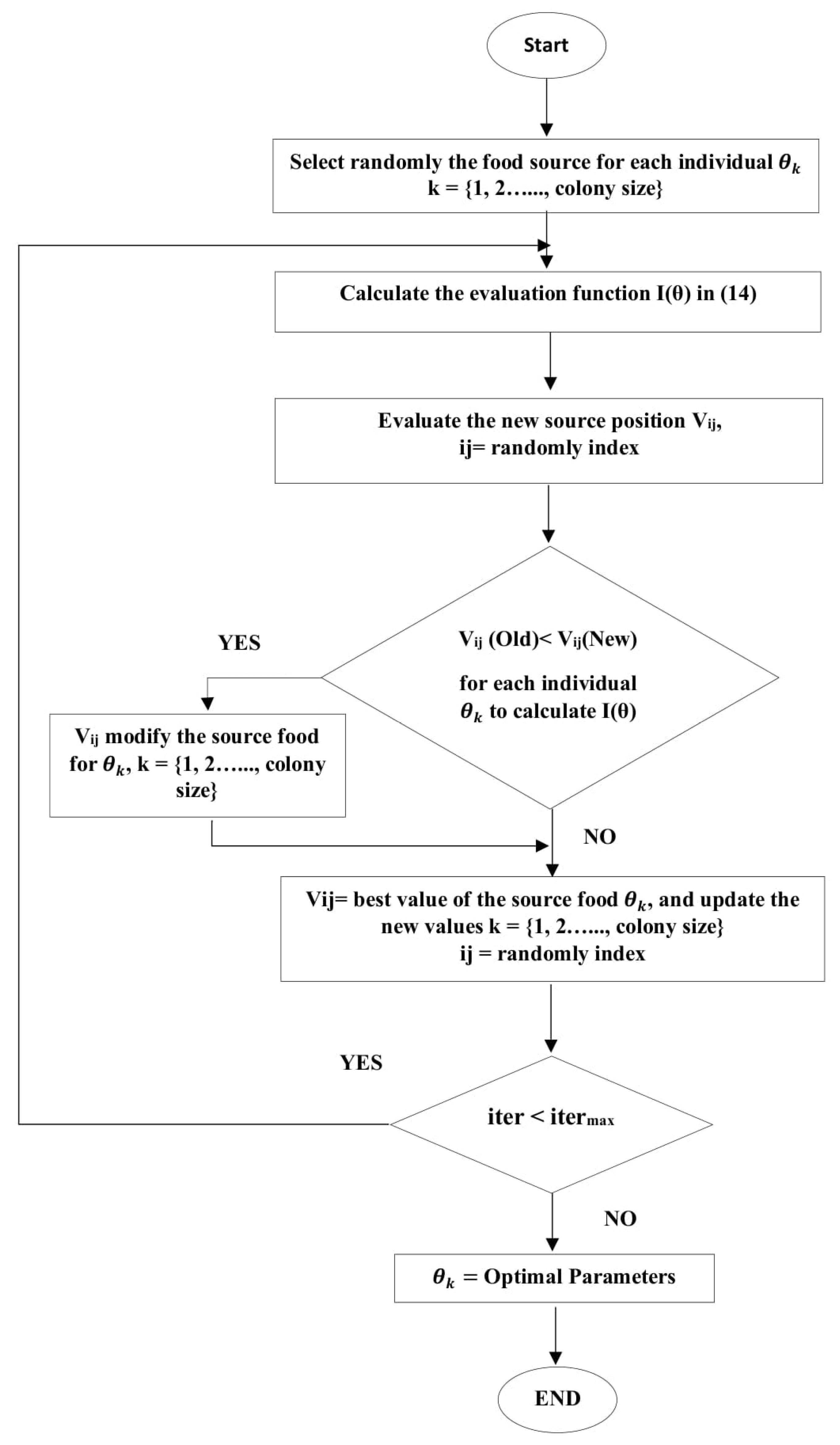
4.1. Explanation Method of H∞ Controller Using ABC
- Randomly select the food source for each individual , where k is the colony size of the ABC algorithm k = {1, 2, ……, colony size (population)}.
- Calculate the values of the evaluation function in Equation (14) as previously explained, and apply the result in the droop control equations.
- Calculate the new value of the source position , where i and j are randomly selected indexes.
- Compare the new value of the source position of each individual with old values according to Equation (3).
- In case the new source food is better than the old source, modify the source food of each individual according to the mathematical equation of the ABC algorithm. If not, the new source is the best value of source food.
- Test the maximum number of iterations; if the number of iterations reaches the maximum, this means that the last value is the optimal controller parameter. If not, repeat the process to evaluate the objective function for , where k = {1, 2…..., colony size}. The algorithm flowchart is shown in Figure 10.
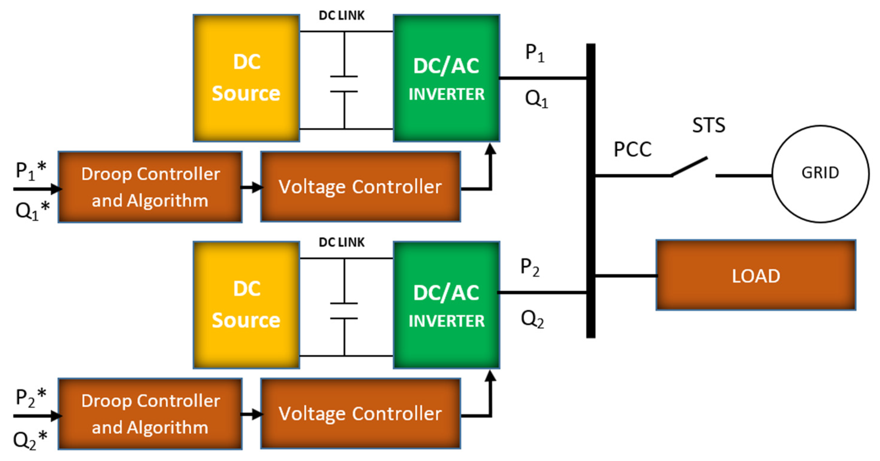
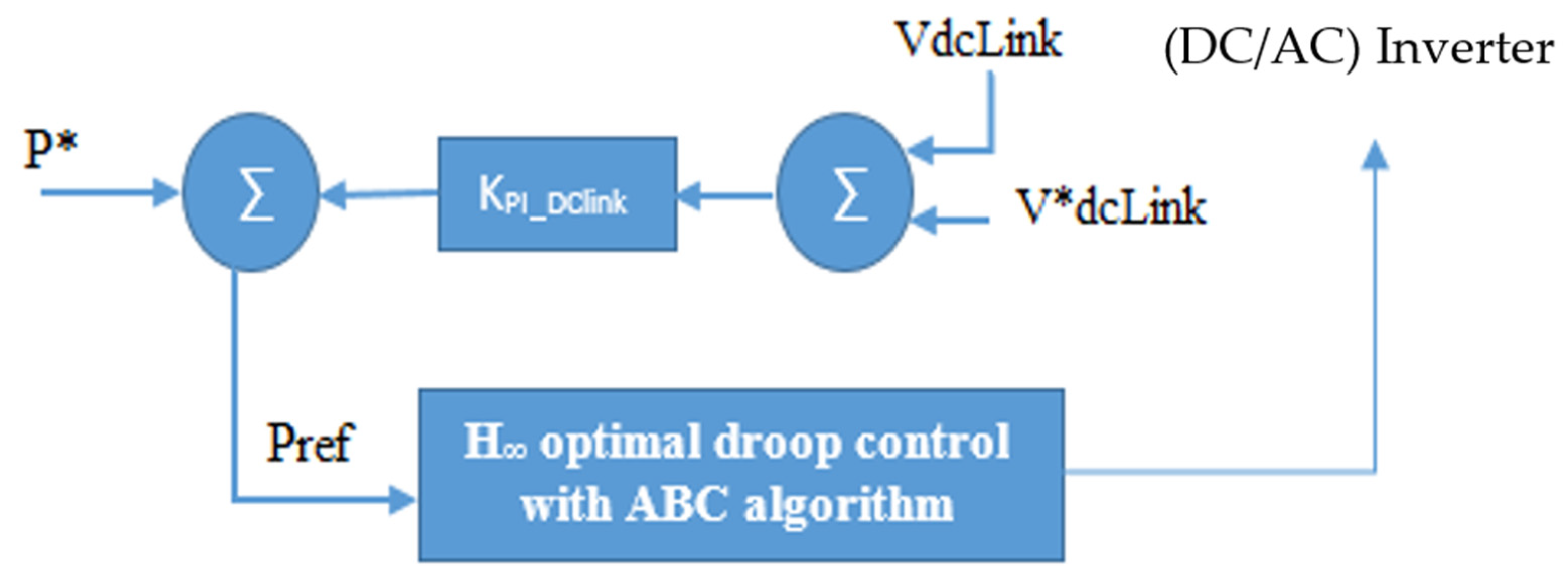
4.2. Inverter’s Power Regulator
- Conventional controller.
- Particle swarm optimization (PSO) algorithm.
- Artificial bee colony algorithm.
- H∞ optimal controller with the ABC algorithm.
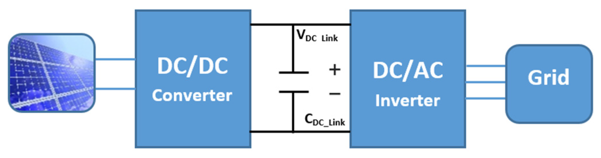
5. DC Link Voltage and Circulating Power of the Inverters
5.1. DC Link Modeling
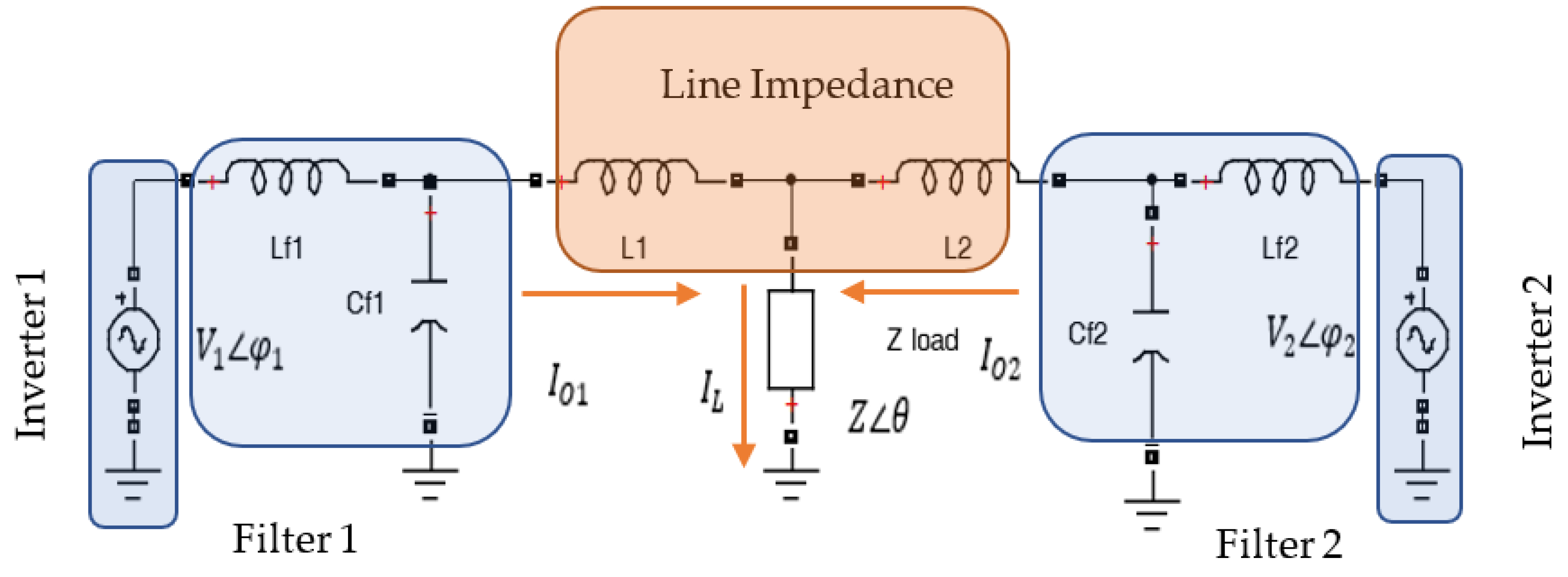
5.2. Power Calculation and Equations of Parallel Inverters
5.3. Design of the DC Link Voltage
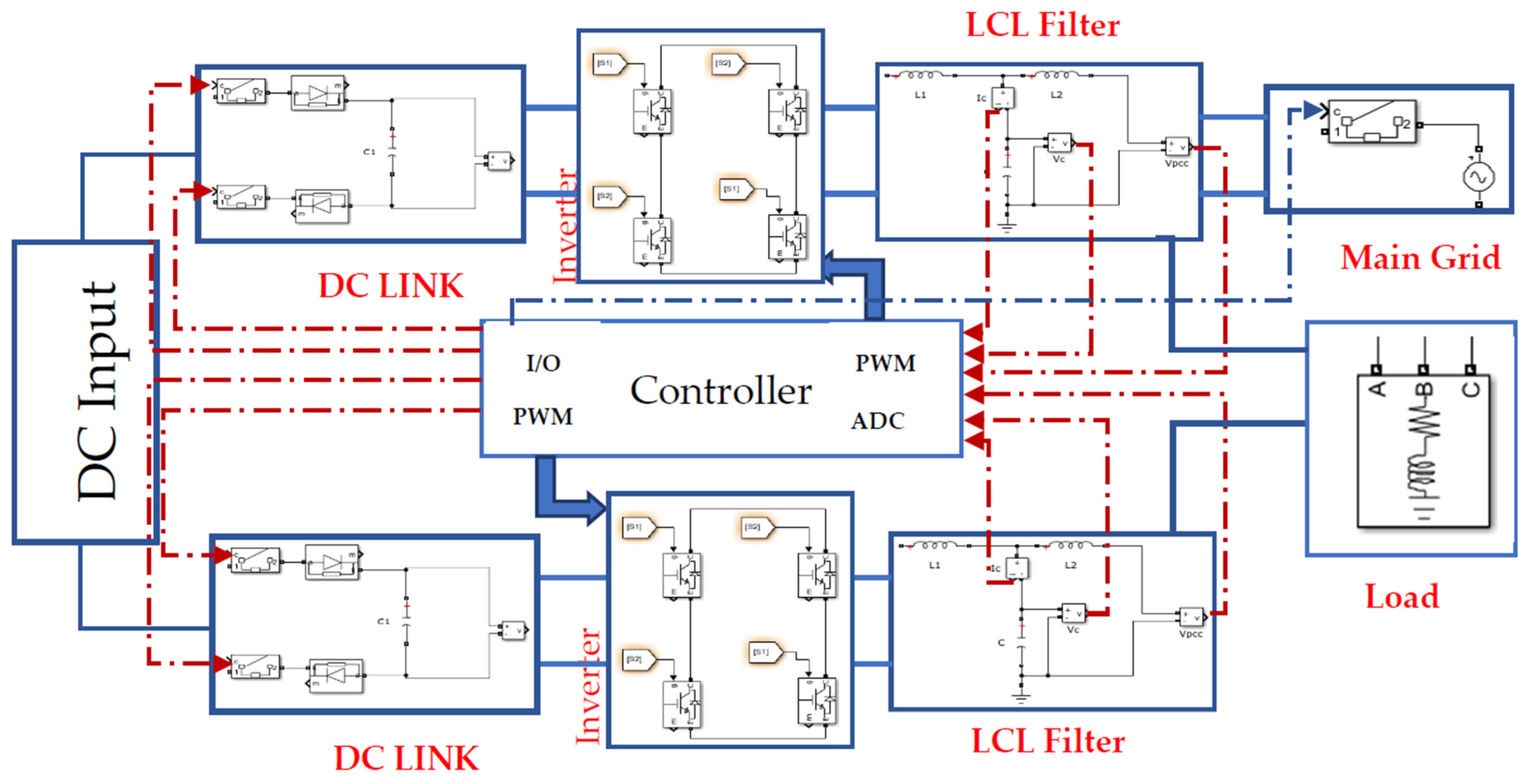
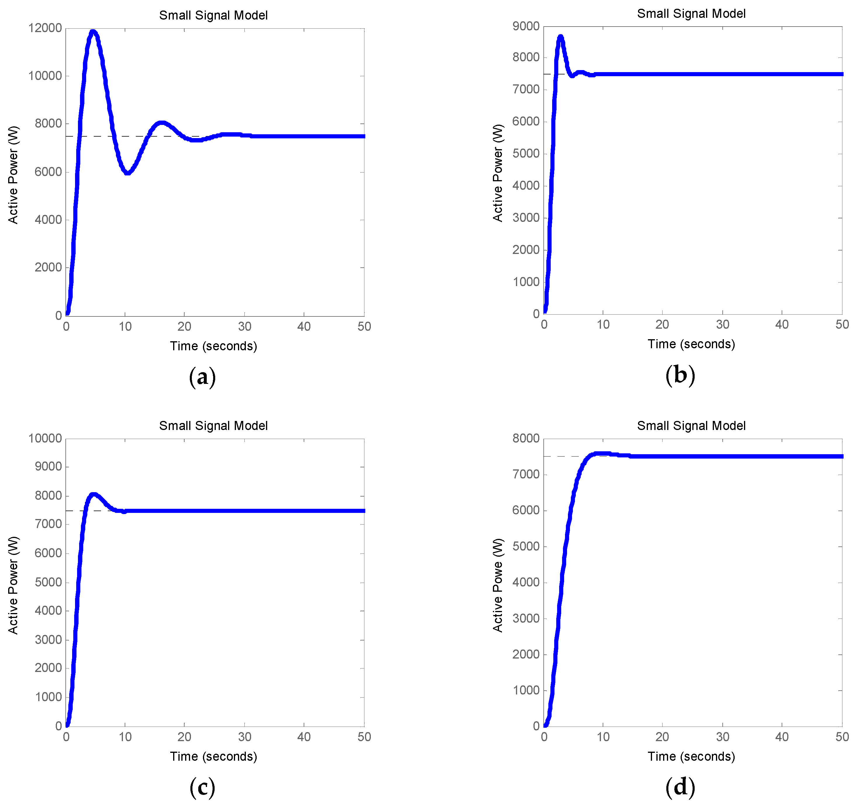
6. Simulation Results and Verification
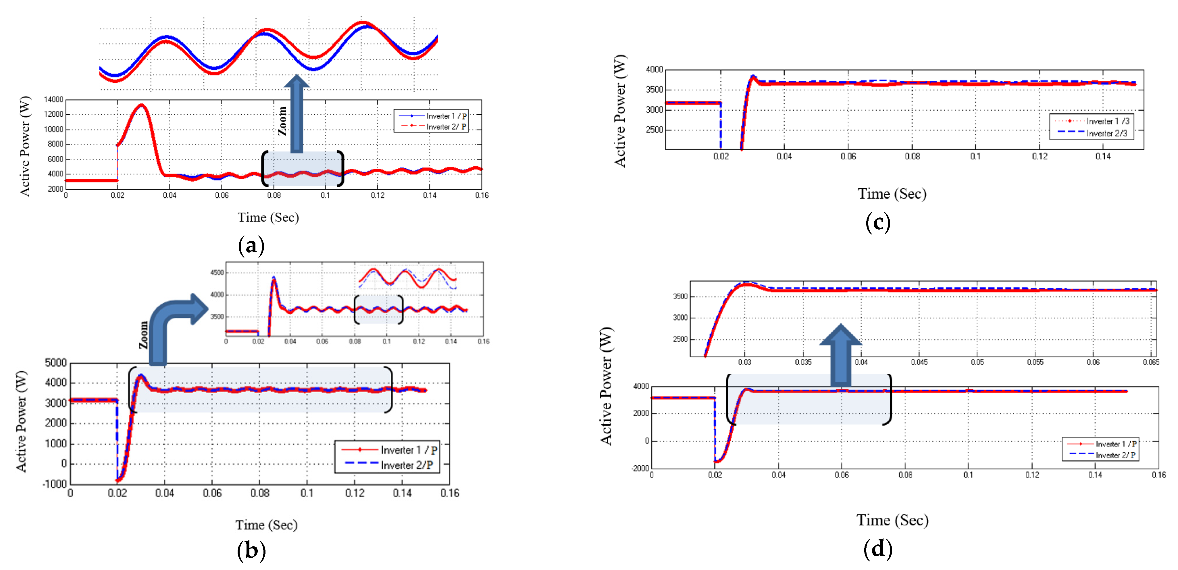
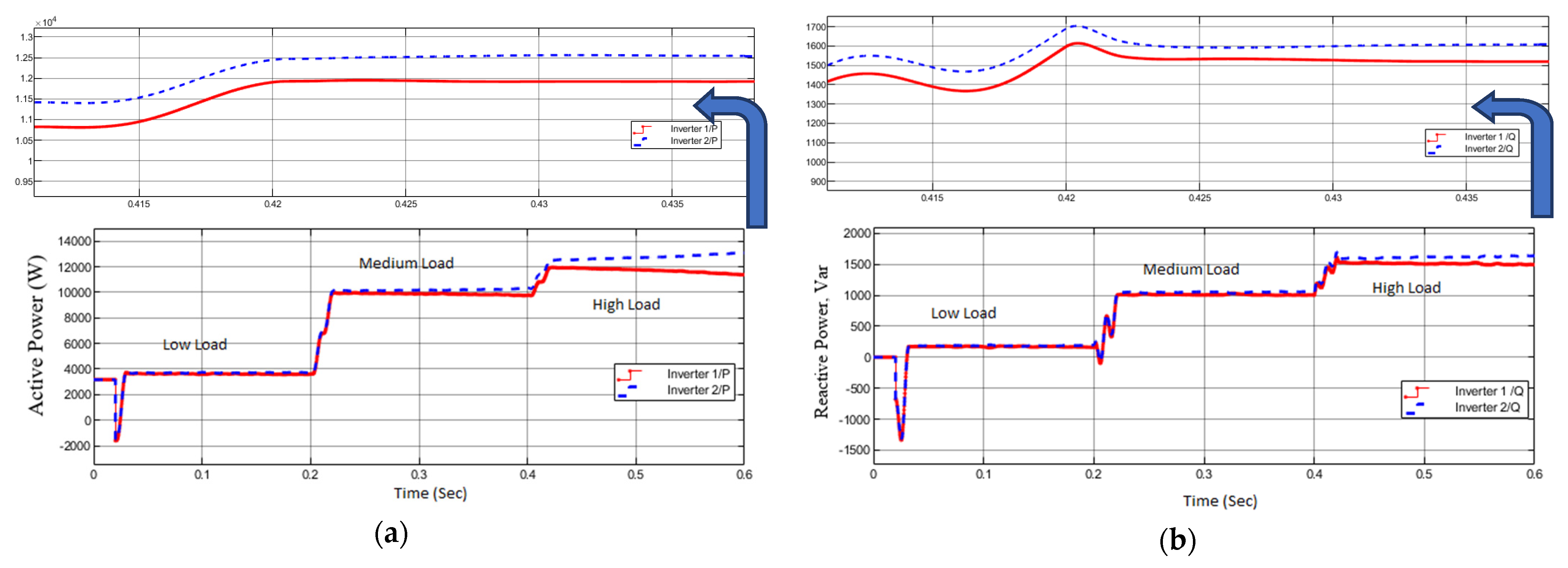
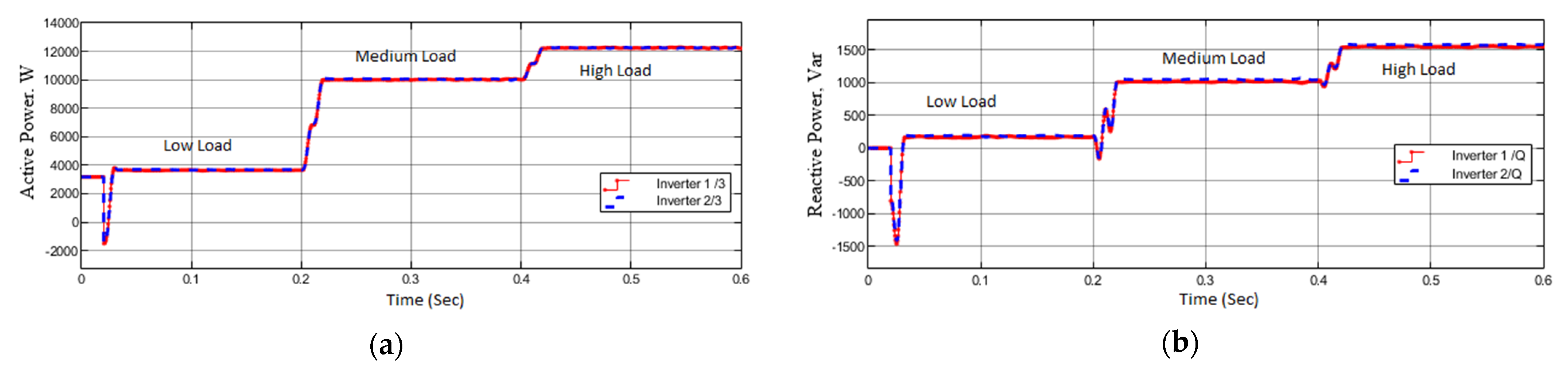
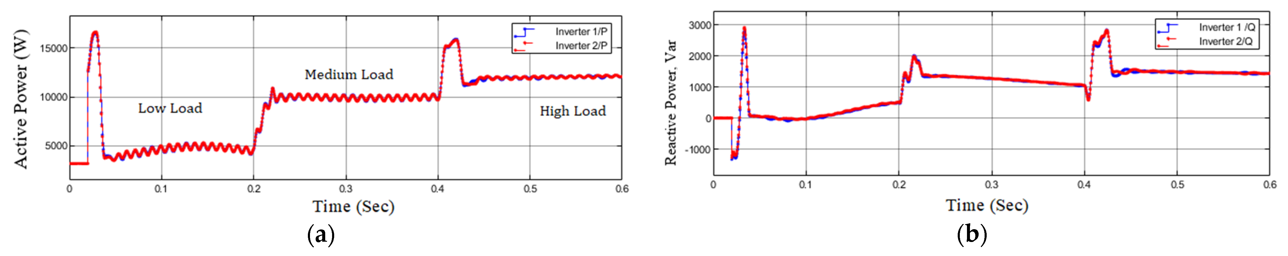
6.1. Active Power Sharing among Two Parallel Inverters
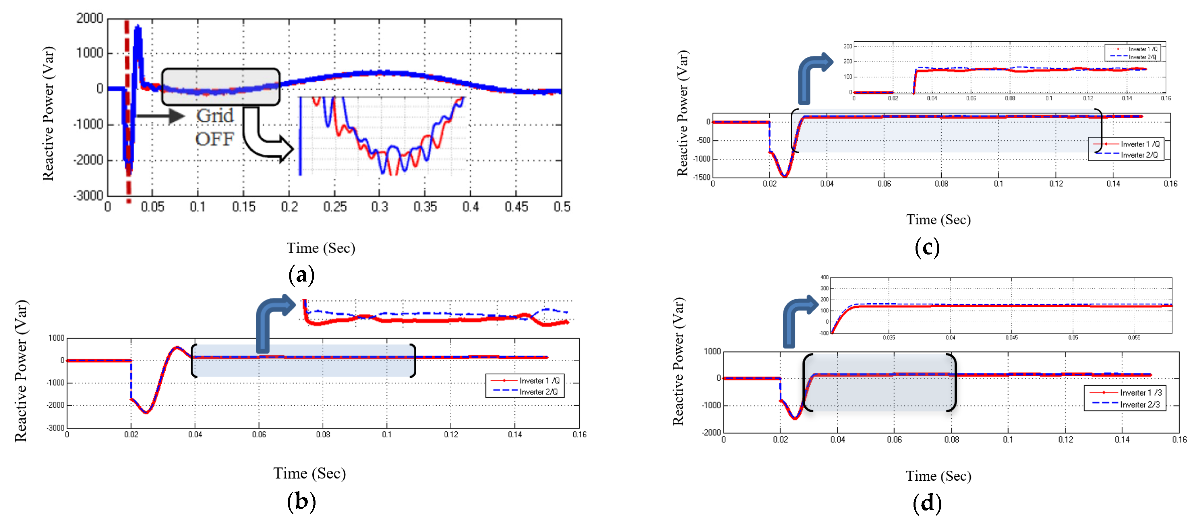
6.2. Reactive Power Sharing among Two Parallel Inverters
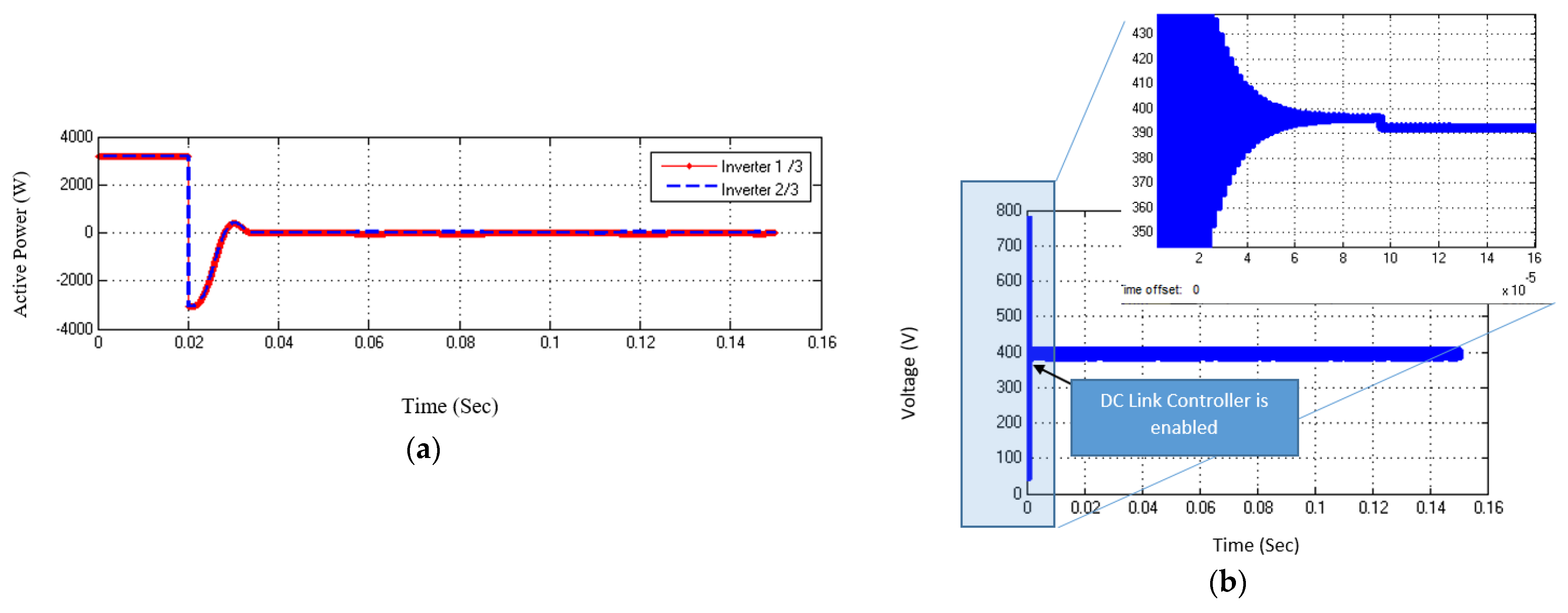
6.3. Result of the DC Link Controller
6.4. Power Sharing Signal Analysis under Variable Loads
7. Conclusions
Author Contributions
Funding
Data Availability Statement
Acknowledgments
Conflicts of Interest
Nomenclature
| P* and Q* | Active and reactive power nominal value |
| P and Q | Active and reactive power actual value |
| Kp and kq | Frequency and voltage droop control gain compensator |
| w* and E* | Frequency and voltage nominal value |
| w and E | Frequency and voltage actual value |
| Vik | The ith particle velocity at kth iteration. |
| Xik | The particle’s current position. The i and k are particle index, and iteration index. |
| Pbest and Pgbest | The particle’s best position and global group’s global best position. |
| r1 and r2 | Random numbers between {0, 1} |
| Vij | A new food source (i, j are random selected index) |
| Xkj | Selected random food source, and k = {1, 2, …, colony size (population)} |
| φij | A random number {−1, 1} |
| G(s) | Uncertain plant of the closed-loop system |
| Yp(t), and R(t) | The output system, and a reference input |
| e(t), and C(s) | An error signal of the closed-loop control system, and the tuning algorithm of PID controller |
| Wd, and Wn | Weighting functions |
| D(t) and N(t) | The disturbance and the noise |
| T(s) and D(s) | Complementary function, and sensitivity function |
| P∞,τ | The robust stability performed by H∞ optimization, and a time constant. |
| OS, tr, ts, ESS, ai | Overshoot, rising time, settling time, steady-state error, weight factor (i = 1, 2 …, 5) |
| I(θ) | The performance for weighting function, θ is the coefficient controller |
| KPID | Kp, KI, and KD are proportional, integral, and derivative controllers |
| β | The phase angle between the output voltage inverter and the Common AC bus |
| VL, Zo, φ | Load voltage, the equivalent output reactance and resistance of each inverter |
| KPE, KPβ, KqE, Kqβ | The coefficients of linearity |
| ΔP and ΔQ | The change output active power and reactive power |
| ΔPavg and ΔQavg | Average values of the change active power and reactive power |
| EDC_Link | The energy absorbed by the DC link capacitor |
| VDC_Link | The voltage drops on the link capacitor |
| CDC_Link | The DC link capacitor |
| ∆VDC_Link | The DC link voltage variation value |
Appendix A. The Change Output Powers of the First and Second Inverters Coefficients
Appendix B
Appendix C
References
- He, J.; Liu, X.; Mu, C.; Wang, C. Hierarchical control of series-connected string converter-based islanded electrical power system. IEEE Trans. Power Electron. 2020, 35, 359–372. [Google Scholar] [CrossRef]
- Wang, C.; Yang, X.; Wu, Z.; Che, Y.; Guo, L.; Zhang, S.; Liu, Y. A highly integrated and reconfigurable microgrid testbed with hybrid distributed energy sources. IEEE Trans. Smart Grid 2016, 7, 451–459. [Google Scholar] [CrossRef]
- Pavon, W.; Inga, E.; Simani, S.; Nonato, M. A Review on Optimal Control for the Smart Grid Electrical Substation Enhancing Transition Stability. Energies 2021, 14, 8451. [Google Scholar] [CrossRef]
- Mohandes, B.; Acharya, S.; El Moursi, M.S.; Al-Sumaiti, A.S.; Doukas, H.; Sgouridis, S. Optimal design of an islanded microgrid with load shifting mechanism between electrical and thermal energy storage systems. IEEE Trans. Power Syst. 2020, 35, 2642–2657. [Google Scholar] [CrossRef]
- Hosseini, S.M.; Carli, R.; Dotoli, M. Robust optimal energy management of a residential microgrid under uncertainties on demand and renewable power generation. IEEE Trans. Autom. Sci. Eng. 2020, 18, 618–637. [Google Scholar] [CrossRef]
- Chiang, H.C.; Jen, K.K.; You, G.H. Improved droop control method with precise current sharing and voltage regulation. IET Power Electron. 2016, 9, 789–800. [Google Scholar] [CrossRef]
- Meng, X.; Liu, J.; Liu, Z. A generalized droop control for grid-supporting inverter based on comparison between traditional droop control and virtual synchronous generator control. IEEE Trans. Power Electron. 2018, 34, 5416–5438. [Google Scholar] [CrossRef]
- Chen, J.; Yue, D.; Dou, C.; Chen, L.; Weng, S.; Li, Y. A Virtual Complex Impedance Based P-V Droop Method for Parallel-Connected Inverters in Low-Voltage AC Microgrids. IEEE Trans. Ind. Inform. 2020, 17, 1763–1773. [Google Scholar] [CrossRef]
- Aderibole, A.; Zeineldin, H.; Al Hosani, M.; El-Saadany, E.F. Demand side management strategy for droop-based autonomous microgrids through voltage reduction. IEEE Trans. Energy Convers. 2018, 34, 878–888. [Google Scholar] [CrossRef]
- Li, Z.; Chan, K.W.; Hu, J.; Guerrero, J.M. Adaptive Droop Control Using Adaptive Virtual Impedance for Microgrids with Variable PV Outputs and Load Demands. IEEE Trans. Ind. Electron. 2020, 68, 9630–9640. [Google Scholar] [CrossRef]
- Pouryekta, A.; Ramachandaramurthy, V.K.; Mithulananthan, N.; Arulampalam, A. Islanding detection and enhancement of microgrid performance. IEEE Syst. J. 2018, 12, 3131–3141. [Google Scholar] [CrossRef]
- Yao, W.; Chen, M.; Matas, J.; Guerrero, J.M.; Qian, Z.-M. Design and analysis of the droop control method for parallel inverters considering the impact of the complex impedance on the power sharing. IEEE Trans. Ind. Electron. 2011, 58, 576–588. [Google Scholar] [CrossRef]
- Dos Santos Neto, P.J.; Dos Santos Barros, T.A.; Silveira, J.P.C.; Ruppert Filho, E.; Vasquez, J.C.; Guerrero, J.M. Power management strategy based on virtual inertia for DC microgrids. IEEE Trans. Power Electron. 2020, 35, 12472–12485. [Google Scholar] [CrossRef]
- Singh, B.; Sharma, R.; Kewat, S. Robust Control Strategies for SyRG-PV and Wind-Based Islanded Microgrid. IEEE Trans. Ind. Electron. 2021, 68, 3137–3147. [Google Scholar] [CrossRef]
- Deng, W.; Dai, N.; Lao, K.-W.; Guerrero, J.M. A Virtual-Impedance Droop Control for Accurate Active Power Control and Reactive Power Sharing Using Capacitive-Coupling Inverters. IEEE Trans. Ind. Appl. 2020, 56, 6722–6733. [Google Scholar] [CrossRef]
- Helmi, A.M.; Carli, R.; Dotoli, M.; Ramadan, H.S. Efficient and Sustainable Reconfiguration of Distribution Networks via Metaheuristic Optimization. IEEE Trans. Autom. Sci. Eng. 2021, 19, 82–98. [Google Scholar] [CrossRef]
- Muhammad, M.A.; Mokhlis, H.; Naidu, K.; Amin, A.; Franco, J.F.; Othman, M. Distribution network planning enhancement via network reconfiguration and DG integration using dataset approach and water cycle algorithm. J. Mod. Power Syst. Clean Energy 2019, 8, 86–93. [Google Scholar] [CrossRef]
- Hamzeh, M.; Mokhtari, H.; Karimi, H. A decentralized self-adjusting control strategy for reactive power management in an islanded multi-bus MV microgrid. Can. J. Electr. Comput. Eng. 2013, 36, 18–25. [Google Scholar] [CrossRef]
- Choudhury, S. A comprehensive review on issues, investigations, control and protection trends, technical challenges and future directions for Microgrid technology. Int. Trans. Electr. Energy Syst. 2020, 30, e12446. [Google Scholar] [CrossRef]
- Ding, W.; Fang, W. Target tracking by sequential random draft particle swarm optimization algorithm. In Proceedings of the 2018 IEEE International Smart Cities Conference (ISC2), Kansas City, MO, USA, 16–19 September 2018; pp. 1–7. [Google Scholar]
- Jouda, M.S.; Kahraman, N. Optimized control and Power Sharing in Microgrid Network. In Proceedings of the 2019 7th International Istanbul Smart Grids and Cities Congress and Fair (ICSG), Istanbul, Turkey, 25–26 April 2019; pp. 129–133. [Google Scholar]
- Bağış, A.; Senberber, H. Modeling of higher order systems using artificial bee colony algorithm. Int. J. Optim. Control Theor. Appl. 2016, 6, 129–139. [Google Scholar] [CrossRef]
- Habib, H.U.R.; Subramaniam, U.; Waqar, A.; Farhan, B.S.; Kotb, K.M.; Wang, S. Energy cost optimization of hybrid renewables based V2G microgrid considering multi objective function by using artificial bee colony optimization. IEEE Access 2020, 8, 62076–62093. [Google Scholar] [CrossRef]
- Chamchuen, S.; Siritaratiwat, A.; Fuangfoo, P.; Suthisopapan, P.; Khunkitti, P. High-Accuracy power quality disturbance classification using the adaptive ABC-PSO as optimal feature selection algorithm. Energies 2021, 14, 1238. [Google Scholar] [CrossRef]
- Hua, H.; Qin, Y.; Geng, J.; Hao, C.; Cao, J. Robust Mixed H 2/H ∞ Controller Design for Energy Routers in Energy Internet. Energies 2019, 12, 340. [Google Scholar] [CrossRef] [Green Version]
- Hayat, R.; Leibold, M.; Buss, M. Robust-Adaptive Controller Design for Robot Manipulators Using the H∞ Approach. IEEE Access 2018, 6, 51626–51639. [Google Scholar] [CrossRef]
- Baburajan, S.; Wang, H.; Kumar, D.; Wang, Q.; Blaabjerg, F. DC-Link Current Harmonic Mitigation via Phase-Shifting of Carrier Waves in Paralleled Inverter Systems. Energies 2021, 14, 4229. [Google Scholar] [CrossRef]
- Jin, Q.; Liu, Q.; Huang, B. Control design for disturbance rejection in the presence of uncertain delays. IEEE Trans. Autom. Sci. Eng. 2015, 14, 1570–1581. [Google Scholar] [CrossRef]
- Rodríguez-Licea, M.-A.; Pérez-Pinal, F.-J.; Nuñez-Perez, J.-C.; Herrera-Ramirez, C.-A. Nonlinear Robust Control for Low Voltage Direct-Current Residential Microgrids with Constant Power Loads. Energies 2018, 11, 1130. [Google Scholar] [CrossRef] [Green Version]
- Ravada, B.R.; Tummuru, N.R. Control of a supercapacitor-battery-PV based stand-alone DC-microgrid. IEEE Trans. Energy Convers. 2020, 35, 1268–1277. [Google Scholar] [CrossRef]
- Magableh, M.A.K.; Radwan, A.; Mohamed, Y.A.-R.I. Assessment and Mitigation of Dynamic Instabilities in Single-Stage Grid-Connected Photovoltaic Systems with Reduced DC-Link Capacitance. IEEE Access 2021, 9, 55522–55536. [Google Scholar] [CrossRef]
- Issa, W.R.; El Khateb, A.H.; Abusara, M.A.; Mallick, T.K. Control strategy for uninterrupted microgrid mode transfer during unintentional islanding scenarios. IEEE Trans. Ind. Electron. 2017, 65, 4831–4839. [Google Scholar] [CrossRef] [Green Version]
- Yan, X.; Cui, Y.; Cui, S. Control Method of Parallel Inverters with Self-Synchronizing Characteristics in Distributed Microgrid. Energies 2019, 12, 3871. [Google Scholar] [CrossRef] [Green Version]


| Method | Control PID Parameters | Step Response Characteristics | ||
|---|---|---|---|---|
| OS % | Ts (S) | Absolute Error | ||
| Conventional | Kp = 0.64 Ki = 0.24 Kd = 0.308 | 58.2 | 23.3 | 25.8 |
| PSO | Kp = 0.9005 Kd = 0.5284 | 15.8 | 4.18 | 15.6004 |
| ABC | Kp = 0.5885 Kd = 0.1988 | 7.41 | 7.24 | 14.2117 |
| ABC with H∞ | Kp = 0.313 Kd = 0.225 | 1.26 | 7 | 10.529 |
| Symbol | Description | Value |
|---|---|---|
| Nominal Value of Active Power for inverter 1 | 10 KW | |
| Nominal Value of Active Power for inverter 2 | 10 KW | |
| Nominal Value of Reactive Power for inverter 1 | 150 Var | |
| Nominal Value of Reactive Power for inverter 2 | 150 Var | |
| Load Active Power | 7500 W | |
| Load Reactive Power | 300 Var | |
| Nominal Voltage | 325 V | |
| Nominal frequency | 50 HZ | |
| VDC_Link | DC link voltage | 400 V |
| Method | Overshoot % | Power Matching among Inverter 1 and Inverter 2 % | ||
|---|---|---|---|---|
| P1 % | P2 % | |||
| DGs Active Power | PSO Droop Control ABC Droop Control H∞ with ABC | 13.33 3.42 1.34 | 16 3.85 1.86 | 81.34 98.165 98.64 |
| DGs Reactive Power | Q1 % | Q2 % | ||
| PSO Droop Control ABC Droop Control H∞ with ABC | 10.33 1.12 0.85 | 15.5 3.34 1.47 | 80.62 93.89 96.77 | |
| Symbol | Description | Value |
|---|---|---|
| PMax | Maximum value of active power for each inverter | 13 KW |
| QMax | Maximum value of reactive power for each inverter | 3.5 KW |
| PL Low | Low load active power | 7 KW |
| QL Low | Low load reactive power | 300 Var |
| PL Medium | Medium load active power | 20 KW |
| QL Medium | Medium load reactive power | 2 KVar |
| PL High | High load active power | 25 KW |
| QL High | High load reactive power | 3 KVar |
| Nominal peak voltage | 325 V | |
| Nominal frequency | 50 HZ | |
| VDC_Link | DC link voltage | 400 V |
Publisher’s Note: MDPI stays neutral with regard to jurisdictional claims in published maps and institutional affiliations. |
© 2022 by the authors. Licensee MDPI, Basel, Switzerland. This article is an open access article distributed under the terms and conditions of the Creative Commons Attribution (CC BY) license (https://creativecommons.org/licenses/by/4.0/).
Share and Cite
Jouda, M.S.; Kahraman, N. Improved Optimal Control of Transient Power Sharing in Microgrid Using H-Infinity Controller with Artificial Bee Colony Algorithm. Energies 2022, 15, 1043. https://doi.org/10.3390/en15031043
Jouda MS, Kahraman N. Improved Optimal Control of Transient Power Sharing in Microgrid Using H-Infinity Controller with Artificial Bee Colony Algorithm. Energies. 2022; 15(3):1043. https://doi.org/10.3390/en15031043
Chicago/Turabian StyleJouda, Mohammed Said, and Nihan Kahraman. 2022. "Improved Optimal Control of Transient Power Sharing in Microgrid Using H-Infinity Controller with Artificial Bee Colony Algorithm" Energies 15, no. 3: 1043. https://doi.org/10.3390/en15031043
APA StyleJouda, M. S., & Kahraman, N. (2022). Improved Optimal Control of Transient Power Sharing in Microgrid Using H-Infinity Controller with Artificial Bee Colony Algorithm. Energies, 15(3), 1043. https://doi.org/10.3390/en15031043