Optimal Sizing of Battery Energy Storage Systems Considering Cooperative Operation with Microgrid Components

Abstract

Battery energy storage systems (BESSs) are key components in efficiently managing the electric power supply and demand in microgrids. However, the BESSs have issues in their investment costs and operating lifetime, and thus, the optimal sizing of the BESSs is one of the crucial requirements in design and management of the microgrids. This paper presents a problem framework and its solution method that calculates the optimal size of the BESSs in a microgrid, considering their cooperative operations with the other components. The proposed framework is formulated as a bi-level optimization problem; however, based on the Karush–Kuhn–Tucker approach, it is regarded as a type of operation scheduling problem. As a result, the techniques developed for determining the operation schedule become applicable. In this paper, a combined algorithm of binary particle swarm optimization and quadratic programming is selected as the basis of the solution method. The validity of the authors’ proposal is verified through numerical simulations and discussion of their results.

1. Introduction

Microgrids are a framework of smart power grids that manage a localized group of electrical power sources and loads, which can be operated in both connected and disconnected to bulk power grids [1,2,3]. In association with the growth in the installation of renewable energy-based variable generation systems (VREs), microgrids are highly expected as some of the most realistic, sustainable power grids, in terms of the efficient use of renewable energy sources (RESs). In fact, extensive studies and developments have been promoted to improve their operations since the early 2000s [4,5], and demonstrative field tests are actively being carried out [6,7].

Generally, components of a microgrid are classified into a controllable and uncontrollable component. The former type consists of controllable power generation systems (CGs) and battery energy storage systems (BESSs). Meanwhile, the latter type includes electrical loads and VREs, which can be treated as one aggregated uncontrollable component in microgrid operations; this is the net load. Operators of the microgrid make an operation schedule of the controllable components, relying on the assumed profiles of the uncontrollable components (or the assumed profile of the net load) in advance, and adjust the schedule by reflecting the actual behavior of the net load. In the process, the BESSs take on an extremely important role that compensates the power surplus or shortage in the microgrid by their charging or discharging function, in addition to contributions to the reduction of operational costs and peak shaving [8,9,10,11]. By contrast, the BESSs, as is well known, have issues in their investment costs and operating lifetime, and these create a bottleneck in design and management of the microgrid. For these reasons, it becomes a crucial requirement to calculate the optimal size of the BESSs in consideration of the operation schedule after the BESS installation, despite difficulties in the operation scheduling [12,13,14].

Focusing on the CGs only, their operation scheduling is formulated as a mixed integer programming (MIP) problem that combines problems of the unit commitment (UC) and the economic load dispatch (ELD). As it is essentially the same as the UC–ELD problem for the thermal power generation units in the bulk power grids, their solution techniques are applicable. Historically, the traditional optimization algorithms, e.g., branch-and-bound (BB) [15,16] and dynamic programming (DP) [17,18], have been used for the solution methods of the UC–ELD problems. Intelligent optimization algorithms, which include genetic algorithms (GAs) [19], simulated annealing (SA) [20,21], and particle swarm optimization (PSO) [22,23], are adopted to the problems, too. Although various algorithms have been applied, there are still none established for the UC–ELD problems, as well as the operation scheduling problems of the CGs.

In microgrids, VREs and BESSs have significant portions in the electrical power source, and we cannot forget their influences on the balancing operations of the power supply and demand. The VREs, whose outputs strongly depend on the weather conditions, increase the uncertainty in the assumed profile of the net load. The BESSs enhance flexibility in the microgrid operations; however, they bring additional variables into the operation scheduling problems, which represent their operational states. Hence practical operation scheduling problems become more complicated than the case when we only treat the UC–ELD problem [24,25,26,27,28]. Similarly, the optimal BESS sizing has often been discussed separately from the optimal operation scheduling in spite of the fact that the size and the operations of the BESSs have influences on each other.

The authors propose a problem framework and its solution method that calculates the optimal size of BESSs, while determining the optimal operation schedule of controllable components in a microgrid. To emphasize the mutual interaction in the optimal sizing and the optimal operation scheduling, the proposed framework is formulated as a bi-level optimization problem. However, in the solution process, the problem is regarded as a type of standard optimization problem under Karush–Kuhn–Tucker (KKT) conditions. In the solution method, a combined algorithm of binary particle swarm optimization (BPSO) and quadratic programming (QP), which is the BPSO–QP [23,28], is applied to the problem framework. This algorithm was originally proposed for operation scheduling problems, but in this paper, it provides both the optimal size of the BESSs and the optimal operation schedule of the microgrid under the assumed profile of the net load. By the BPSO–QP application, we can localize influences of the stochastic search of the BPSO into the generating process of the UC candidates of CGs. Through numerical simulations and discussion on their results, the validity of the proposed framework and the usefulness of its solution method are verified.

2. Problem Formulation

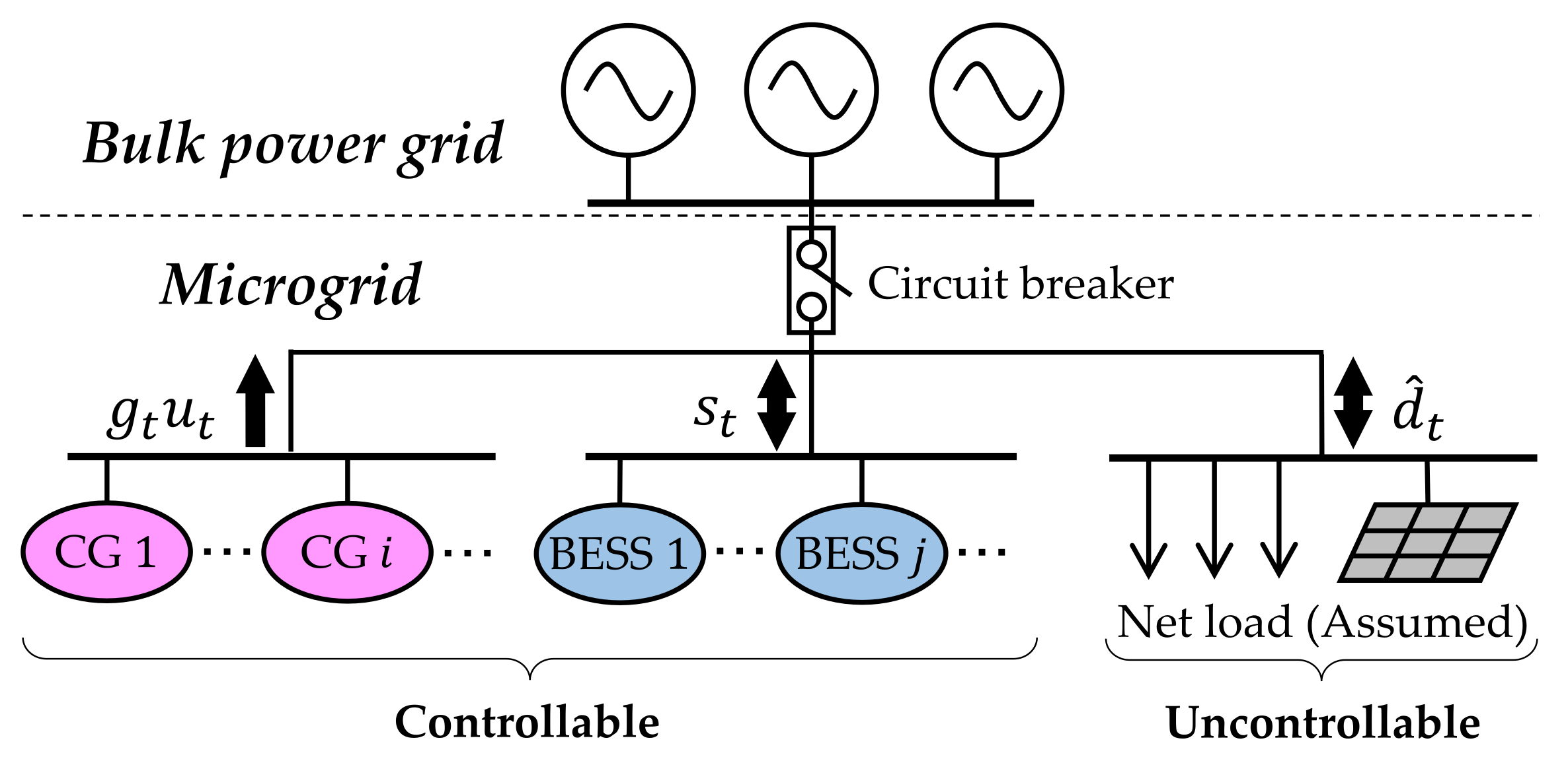
As illustrated in Figure 1, there are four types in the microgrid components: (1) CGs, (2) BESSs, (3) electrical loads, and (4) VREs. Controllable loads can be regarded as a type of BESSs. The CGs and the BESSs are controllable, while the electrical loads and the VREs are uncontrollable that can be aggregated as the net load. Operation scheduling of the microgrids is represented as the problem of determining a set of the start-up/shut-down times of the CGs, their output shares, and the charging/discharging states of the BESSs. In operation scheduling problems, we normally set the assumption that the specifications of the CGs and the BESSs, along with the profiles of the electrical loads and the VRE outputs, are given.

If the power supply and demand cannot be balanced, an extra payment, which is the imbalance penalty, is required to compensate the resulting imbalance of power in the grid-tie microgrids, or the resulting outage in the stand-alone microgrids. Since the imbalance penalty is extremely expensive, the microgrid operators secure the reserve power to prevent any unexpected additional payments. This is the reason why the operational margin of the CGs and the BESSs is emphasized in the operation scheduling. Moreover, the operational margin of the BESSs strongly depends on their size, and therefore, it is crucially required to calculate the appropriate size of the BESSs, considering their investment costs and the contributions by their installation.

To simplify the discussion, the authors mainly focus on a stand-alone microgrid and treat the BESSs as an aggregated BESS. The optimization variables are defined as:

$$Q\in {ℝ}_0^{+},$$

(1)

$$u_{i,t}\in \left\{0, 1\right\}, \mathrm{for} \forall i, \forall t,$$

(2)

$$g_{i,t}\in \left[G_i^{\min },G_i^{\max }\right], \mathrm{for} \forall i, \forall t,$$

(3)

$$s_t\in \left[S^{\min },S^{\max }\right], \mathrm{for} \forall t.$$

(4)

The traditional frameworks of the operation scheduling normally require accurate information for the uncontrollable components; however, this is impractical in the stage of design of the microgrids. The only available information is the assumed profile of the net load (or the assumed profiles of the uncontrollable components) including the uncertainty. The authors define the assumed values of the net load and set their likely ranges as:

$${\widehat{d}}_t\in \left[d_t^{\min },d_t^{\max }\right], \mathrm{for} \forall t.$$

(5)

The target problem is to determine the set of $\left(Q,u,g,s\right)$ in terms of minimizing the sum of investment costs of the newly installing BESSs, $f_1\left(Q\right)$, and operational costs of the microgrid after their installation, $f_2\left(u,g,s\right)$. Based on the framework of bi-level optimization, the target problem is formulated as follows:

Upper-level problem:

$$\underset{u,g,s}{\min }\left[f_1\left(Q\right) + f_2\left(u,g,s\right)\right],$$

(6)

$$\mathrm{s}.\mathrm{t}.\hspace{1em}{\sum }_{i=1}^{NG}{g}_{i,t}{u}_{i,t}+s_t={\widehat{d}}_t, \mathrm{for} \forall t,$$

(7)

$$\mathrm{If} 0<u_{i,t}^{\mathrm{on}}<U{T}_i \mathrm{then} u_{i,t}=1; \mathrm{If} 0<u_{i,t}^{\mathrm{off}}<D{T}_i \mathrm{then} u_{i,t}=0, \mathrm{for} \forall i, \forall t,$$

(8)

$$\Delta G_i^{-}\le g_{i,t}-g_{i,t-1}\le \Delta G_i^{+}, \mathrm{for} \forall i, \forall t,$$

(9)

$$\begin{gathered} g_{i,t}^{\min }\le g_{i,t}\le g_{i,t}^{\max }, \mathrm{for} \forall i, \forall t. \\ (g_{i,t}^{\max }=\min \left(G_i^{\max },g_{i,t-1}+\Delta G_i^{+}\right); g_{i,t}^{\min }=\max \left(G_i^{\min },g_{i,t-1}+\Delta G_i^{-}\right).) \end{gathered}$$

(10)

The detailed definitions of $f_1$ and $f_2$ are as shown below:

$$f_1\left(Q\right) =\psi Q,$$

(11)

$$f_2\left(u,g,s\right)={\sum }_{t=1}^T{\sum }_{i=1}^{NG}\left[({\alpha }_i+{\beta }_i{g}_{i,t}+{\gamma }_i{g}_{i,t}^2)u_{i,t}+{\delta }_i{u}_{i,t}\left(1-u_{i,t-1}\right)\right].$$

(12)

Lower-level problem:

$$\underset{Q}{\min }{f}_1\left(Q\right),$$

(13)

$$\mathrm{s}.\mathrm{t}. {\xi }^{\mathrm{low}}Q\le q_t\le {\xi }^{\mathrm{up}}Q, \mathrm{for} \forall t, (q_t=q_{t-1}-s_t.)$$

(14)

$$\begin{gathered} s_t^{\min }\le s_t\le s_t^{\max }, \mathrm{for} \forall t, \\ (s_t^{\max }=\min \left(S^{\max },\left(q_{t-1}-{\xi }^{\mathrm{low}}Q\right)\right); s_t^{\min }=\max \left(S^{\min },\left(q_{t-1}-{\xi }^{\mathrm{up}}Q\right)\right).) \end{gathered}$$

(15)

$$d_t^{\max }\le \left({\sum }_{i=1}^{NG}{g}_{i,t}^{\max }{u}_{i,t}\right)+s_t^{\max }; \left({\sum }_{i=1}^{NG}{g}_{i,t}^{\min }{u}_{i,t}\right)+s_t^{\min }\le d_t^{\min }, \mathrm{for} \forall t.$$

(16)

In the upper-level problem, Equation (7) represents the balancing constraint of the power supply and demand, and the specifications of the CGs are reflected into the constraints of Equations (8)–(10). Meanwhile, in the lower-level problem, the specifications of the aggregated BESS are expressed with Equations (14) and (15), and the operational margin of the microgrid is secured by Equation (16).

As shown in Equations (6)–(12), the upper-level problem is similar to the operation scheduling problems because the function $f_1$ is treated as though it is a constant. However, the value of $f_1$ is unknown until we solve the lower-level problem, and the values in $s$ are constrained by the value of $Q$. In addition, the optimal size of the aggregated BESS, $Q^{*}$, can be determined only after finding the optimal operation schedule, $\left(u^{*},g^{*},s^{*}\right)$, from the viewpoints of the operational reliability and the economic efficiency. By the mutual interaction in the problems, the target optimization problem becomes complicated, as compared to operation scheduling problems.

In the problem framework, we can treat Equations (8) and (9) as inactive constraints if the time interval and the ramp-up and the ramp-down specifications of the CGs, $\Delta t$, $\Delta G_i^{+}$, and $\Delta G_i^{-}$, satisfy the conditions of Equations (17) and (18) [23,29]. Similarly, the calculations of $g_{i,t}^{\max }$ and $g_{i,t}^{\min }$ are unnecessary in Equation (10) because their values are equal to $G_i^{\max }$ and $G_i^{\min }$, respectively. In other words, this constraint can be integrated into the definition of Equation (3). The conditions Equations (17) and (18) are often satisfied in the operation scheduling of microgrids, and for this reason, the authors remove the constraints Equations (8)–(10) from our discussion.

$$\Delta t\ge U{T}_i+D{T}_i, \mathrm{for} \forall i,$$

(17)

$$\Delta G_i^{+}\ge G_i^{\max }-G_i^{\min }; \Delta G_i^{-}\le G_i^{\min }-G_i^{\max }, \mathrm{for} \forall i.$$

(18)

3. Solution Method

Bi-level optimization is a special form of optimization problem and appears in various models of economics, game theory, and mathematical physics [30]. Its typical applications are found in equilibrium models and in semi-infinite programming [31,32]. From a topological viewpoint, the bi-level optimization is more complicated than standard optimization problems.

In this paper, the KKT approach is applied to the target problem, and then the problem is treated as a type of standard optimization problem. The KKT approach is a methodology that finds the (local) minimizers of the original bi-level optimization problem by computing the (local) minimizers of the relaxation problem [33,34]. To apply the KKT approach, the definition of Equation (4) is converted in accordance with the specifications of the BESSs into:

$$s_t\in \left[-\frac{Q}{\eta },\frac{Q}{\eta }\right], \mathrm{for} \forall t.$$

(19)

By using Equation (19), the variables $s_t^{\max }$ and $s_t^{\min }$ in Equations (15) and (16) are replaced with:

$$s_t^{\max }=\min \left(\frac{Q}{\eta },\left(q_0-{\sum }_{\tau =1}^{t-1}{s}_{\tau }-{\xi }^{\mathrm{low}}Q\right)\right); s_t^{\min }=\max \left(-\frac{Q}{\eta },\left(q_0-{\sum }_{\tau =1}^{t-1}{s}_{\tau }-{\xi }^{\mathrm{up}}Q\right)\right),$$

(20)

where $q_0$ is the initial state of charge (SOC) of the aggregated BESS.

Owing to the representation, all constraints in the lower-level problem become the BESS size-dependent ones. Now, we set the functions ${\phi }_l\left(Q\right)$, of which $l$ is the numbers ($l=1,2,3$) sequentially assigned to the constraints Equations (14)–(16). The lower-level problem is a linear programming (LP) problem, and it can be reformulated in the style of the KKT approach as:

$$\nabla f_1\left(Q^{*}\right)+{\sum }_{l=1}^3{\lambda }_l\nabla {\phi }_l\left(Q^{*}\right)=0,$$

(21)

$${\lambda }_l\ge 0, \mathrm{for} \forall l,$$

(22)

$${\phi }_l\left(Q^{*}\right)\le 0, \mathrm{for} \forall l,$$

(23)

$${\lambda }_l{\phi }_l\left(Q^{*}\right)=0, \mathrm{for} \forall l,$$

(24)

where ${\lambda }_l$ is the Lagrange multipliers in the lower-level problem.

By the reformulation, the KKT approach becomes applicable and integrates the lower-level problem to the constraints of the upper-level problem as the set of Equations (21)–(24). Therefore, we can treat the bi-level optimization as the single-level optimization problem whose objective function is Equation (25) and constraints are Equations (7)–(10) and Equations (21)–(24). For further details of the KKT approach, refer to the references.

$$\underset{Q,u,g,s}{\min }\left[f_1\left(Q\right)+f_2\left(u,g,s\right)\right],$$

(25)

The reformulated problem is an extended framework of the operation scheduling, which determines the discrete variables, $u$, and the set of continuous variables, $\left(Q,g,s\right)$. Hence, we can apply the solution methods developed for operation scheduling problems. In this paper, the BPSO–QP is selected as the basis of the solution method for the reformulated problem.

3.1. Activation of Quadratic Programming

To improve compatibility between the target problem and its solution method, the authors redefine the optimization variables Equations (2)–(4) or Equations (2), (3) and (19) as Equations (26) and (27), and then, replace the function Equation (12) with Equation (28).

$$u_{k,t}^{\prime }\in \left\{0, 1\right\}, \mathrm{for} \forall k, \forall t,$$

(26)

$$g_{k,t}^{\prime }\in \left[{G^{\prime }}_k^{\min },{G^{\prime }}_k^{\max }\right], \mathrm{for} \forall k, \forall t,$$

(27)

$$f_2^{\prime }\left(u^{\prime },g^{\prime }\right)={\sum }_{t=1}^T{\sum }_{k=1}^{NG+1}\left[\left({\alpha }_k^{\prime }+{\beta }_k^{\prime }{g}_{k,t}^{\prime }+{\gamma }_k^{\prime }{\left(g_{k,t}^{\prime }\right)}^2\right)u_{k,t}^{\prime }+{\delta }_k^{\prime }{u}_{k,t}^{\prime }\left(1-u_{k,t-1}^{\prime }\right)\right],$$

(28)

where $k$ is the number assigned to the controllable components ($k=1,2,\dots ,NG+1$); $u_{k,t}^{\prime }$ is the ON/OFF state variable of the controllable component $k$ (ON: $1$, OFF: $0$), which is an element of the vectors $u_t^{\prime }$ and $u^{\prime }$; $g_{k,t}^{\prime }$ is the output of the controllable component $k$, which is an element of the vectors $g_t^{\prime }$ and $g^{\prime }$; ${G^{\prime }}_k^{\max }$ and ${G^{\prime }}_k^{\min }$ are the maximum and the minimum outputs of the controllable component $k$; ${\alpha }_k^{\prime }$, ${\beta }_k^{\prime }$, and ${\gamma }_k^{\prime }$ are the coefficients for fuel cost function of the controllable component $k$; ${\delta }_k^{\prime }$ is the sum of start-up cost of the controllable component $k$.

In Equations (26)–(28), the $\left(NG+1\right)$-th component represents the aggregated BESS ($s_t=g_{N+1,t}^{\prime }{u}_{N+1,t}^{\prime }$; $S^{\max }={G^{\prime }}_{NG+1}^{\max }$; $S^{\min }={G^{\prime }}_{NG+1}^{\min }$). The variables $u_{NG+1,t}^{\prime }$ are the dummy variables whose values are 1 in each time slot (always ON). The values of ${\alpha }_{NG+1}^{\prime }$, ${\beta }_{NG+1}^{\prime }$, ${\gamma }_{NG+1}^{\prime }$ and ${\delta }_{NG+1}^{\prime }$ are set all to zero because the operational cost of the BESS, as shown in Section 2, is expressed with the change of CGs’ operational costs. By these settings, the target problem can be relaxed as a quadratic optimization problem if the values of $u^{\prime }$ are specified. That is, the QP solvers become applicable after generating $u^{\prime }$, and there is no need to discern the difficulty in determining continuous variables.

3.2. Application of Binary Particle Swarm Optimization

When we apply the QP, the dimensions of the solution space are reduced from $\left(Q,u, g,s\right)$ to $u^{\prime }$. However, there is still difficulty in finding the optimal UC solution among a huge number of possible UC candidates [23,28,29]. In this paper, a PSO is used only for generating the feasible UC candidates.

The standard PSO is a population-based stochastic algorithm that iteratively searches the solution space while improving a given measure of solution quality [35], which is the fitness function. Until a termination condition is met, an initial set of randomly generated solutions (initial swarm) updates the position in the solution space towards the globally optimal solution. All members of the swarm (particles) share their information for the solution space during the searching process. Each particle $m$ ($m=1,2,\dots ,M$) has a position $x_{m,n}$ and a velocity $v_{m,n}$ in the iteration $n$ ($n=1,2,\dots ,N$), and these are updated as:

$$x_{m,n}=x_{m,n-1}+v_{m,n}, \mathrm{for} \forall m, \forall n,$$

(29)

$$v_{m,n+1}={\omega }_n{v}_{m,n}+{\theta }_1{r}_1\left[x_m^{*}-x_{m,n}\right]+{\theta }_2{r}_2\left[\left(\underset{m}{\min }{x}_m^{*}\right)-x_{m,n}\right], \mathrm{for} \forall m, \forall n,$$

(30)

where $x_m^{*}$ is the personal best for the particle $m$ (pbest); $\underset{m}{\min }{x}_m^{*}$ is the best in the swarm (gbest).

The positions of the particles, $x_{m,n}$, are defined as the UC candidates, ${\left(u^{\prime }\right)}_{m,n}$, and the fitness function is defined as:

$$f=f_1\left(Q\right)+f_2^{\prime }\left(u^{\prime },g^{\prime }\right)+\nu VIO,$$

(31)

where $\nu$ is the penalty factor ($f_1+f_2^{\prime }\ll \nu VIO$); $VIO$ is the weighted sum of the constraint violations.

Although the PSO has succeeded in many continuous problems, there remain some difficulties in treating discrete optimization problems [36]. Therefore, a strategy of BPSO is adopted in the proposed solution method as shown below:

$$\mathrm{If} 0.5<\frac{1}{1+\exp \left(-u_{k,t}^{\prime }\right)} \mathrm{then} u_{k,t}^{\prime }=1, \mathrm{else} u_{k,t}^{\prime }=0, \mathrm{for} k\le NG, \forall t.$$

(32)

If we focus on the grid-tie microgrids, the penalty term in (31) is replaced with the assumable imbalance penalty, paying for the bulk power grid [23].

3.3. Approximation of Outputs of Controllable Power Generation Systems

By applying the QP, we can localize influences of the stochastic search of the intelligent optimization algorithms into the generating process of the UC candidates. On the other hand, the QP application often leads to impractical computational time depending on the number of the optimization variables or the length of the target period (the value of $T$). To relax this issue, a strategy that approximates the CG outputs [37] is applied.

As opposed to the bulk power grids, the number of the CGs in a microgrid is so small that we can generate all hourly, selectable UC candidates. For example, with five CGs, the number of selectable UC candidates is 2⁵ (=32) in one time slot, and these are common in each time slot. In the approximation strategy, first, the hourly UC candidates are enumerated completely. Associating with the enumerated hourly UC candidates, next, the sets of the optimal output shares and their fuel costs are calculated by the QP within the possible output range of the operating CGs. By using the non-linear regression, finally, the calculated sets of the fuel costs are independently approximated as the fuel functions, with respect to the UC candidates.

According to the procedure, we replace Equation (27) or Equation (3), Equations (7) and (16) with Equations (33)–(35), respectively.

$$h_{u_t^{\prime }}\in \left[H_{u_t^{\prime }}^{\min },H_{u_t^{\prime }}^{\max }\right], \mathrm{for} \forall t, (H_{u_t^{\prime }}^{\max }={\sum }_{k=1}^{NG}{G^{\prime }}_k^{\max }{u}_{k,t}^{\prime }; H_{u_t^{\prime }}^{\min }={\sum }_{i=1}^{NG}{G^{\prime }}_k^{\min }{u}_{k,t}^{\prime }.)$$

(33)

$$h_{u_t^{\prime }}={\widehat{d}}_t-s_t, \mathrm{for} \forall t, (s_t=g_{N+1,t}^{\prime }{u}_{N+1,t}^{\prime })$$

(34)

$$d_t^{\max }\le H_{u_t^{\prime }}^{\max }+s_t^{\max }; H_{u_t^{\prime }}^{\min }+s_t^{\min }\le d_t^{\min }, \mathrm{for} \forall t,$$

(35)

where $h_{u_t^{\prime }}$ is the sum of outputs of the operating CGs ($={\sum }_{k=1}^{NG}{g}_{k,t}^{\prime }{u}_{k,t}^{\prime }$).

In addition, the operational cost function in Equation (31) can be converted into:

$$f_2^{″}\left(u^{\prime },s\right)={\sum }_{t=1}^T\left(A_{u_t^{\prime }}+B_{u_t^{\prime }}{h}_{u_t^{\prime }}+C_{u_t^{\prime }}{\left(h_{u_t^{\prime }}\right)}^2+D_{u_t^{\prime }}\right),$$

(36)

where $A_{u_t^{\prime }}$, $B_{u_t^{\prime }}$, and $C_{u_t^{\prime }}$ are the coefficients of approximated fuel cost functions associating with the vector $u_t^{\prime }$; $D_{u_t^{\prime }}$ is the sum of start-up costs of newly starting-up CGs ($={\sum }_{k=1}^{NG}{\delta }_k^{\prime }{u}_{k,t}^{\prime }\left(1-u_{k,t-1}^{\prime }\right)$).

As shown in Equations (33)–(36), the CG outputs, $g_{k,t}^{\prime }$ ($k\le NG$) (or $g_{i,t}$ for $\forall i$), are linked to the UC candidates. In addition, the approximation can be completed for all selectable UC candidates as a preprocessing of the BPSO–QP. These indicate that we can remove the CG outputs from the optimization variables in the process of the solution method, and thus, reduce the computational cost in the calculation of Equation (31) (iterative calculation of the ELD). For further details of this strategy, refer to the reference.

4. Numerical Simulations and Discussion on Their Results

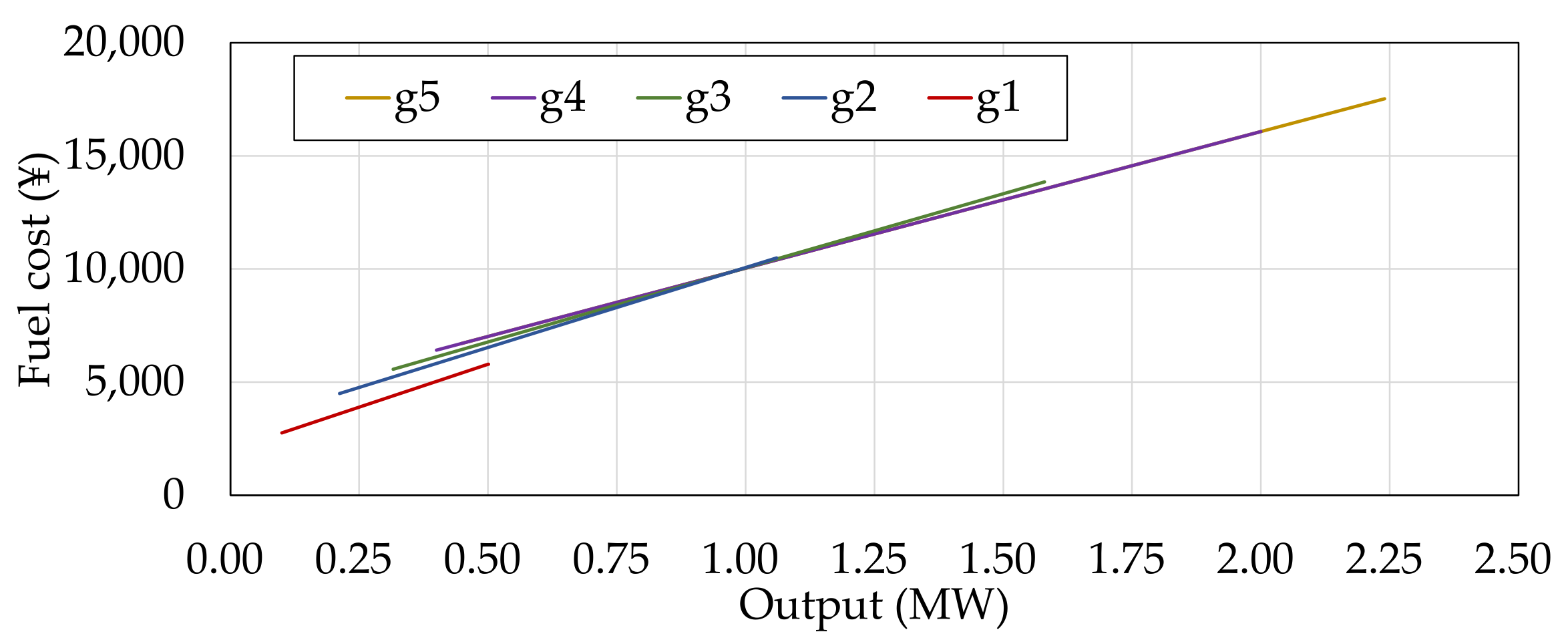
To verify the validity of the authors’ proposal, numerical simulations were carried out on the microgrid model illustrated in Figure 1. To specify the discussion on the numerical simulation results, the target period was set to 24 h ($T=24$), and its interval was set to 1 h ($t=1,\cdots ,24$). The microgrid components were set as five CGs, one aggregated BESS, one aggregated electrical load, and one aggregated photovoltaic generation system (PV). Specifications of the CGs are summarized in

Table 1. Specifications of CGs. “¥” means “any currency unit is applicable”.

$\mathit{i}$	${\mathit{\alpha }}_{\mathit{i}} (\yen )$	${\mathit{\beta }}_{\mathit{i}} (\yen /\mathbf{MW})$	${\mathit{\gamma }}_{\mathit{i}} (\yen /{\mathbf{MW}}^2)$	${\mathit{\delta }}_{\mathit{i}} (\yen )$	${\mathit{G}}_{\mathit{i}}^{\mathbf{max}} \left(\mathbf{MW}\right)$	${\mathit{G}}_{\mathit{i}}^{\mathbf{min}} \left(\mathbf{MW}\right)$
1	9	7500	2000	400	0.500	0.100
2	8	7000	3000	600	1.060	0.212
3	7	6500	3500	700	1.580	0.316
4	6	6000	4000	800	2.000	0.400
5	6	6000	4000	800	2.240	0.448

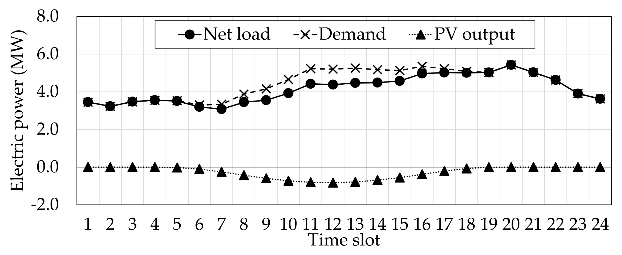
and Figure 2, and the profile of the assumed net load is displayed in Figure 3. These were made with reference to [6,7,37,38]. The unit price of the aggregated BESS, $\psi$, was set to 20,000\/kWh (“\” means “any currency unit is applicable”) [39,40], and the operating lifetime was assumed to 10 years. According to these conditions, the investment cost of the aggregated BESS was converted into the daily one. In the operation scheduling, the authors set the values of ${\xi }^{\mathrm{up}}$ and ${\xi }^{\mathrm{low}}$ to 0.9 and 0.3, and the hour rate $\eta$ to 1.0, respectively. The initial SOC level of the aggregated BESS was set to 60% of its capacity, and the SOC level had to be returned to the original level until the end of the scheduling period. That is, the optimal operation schedule must satisfy the following additional constraints:

$$q_0=q_{24}=0.6Q.$$

(37)

By preliminary trial and error, parameters of the BPSO were respectively set as the following: the total number of particles $M$ is 100, the maximum iteration $N$ is 1000, the initial and the final inertia weight factors ${\omega }_1$ and ${\omega }_{1000}$ are 0.70 and 0.95, and the cognitive factors ${\theta }_1$ and ${\theta }_2$ are 1.6 and 2.0.

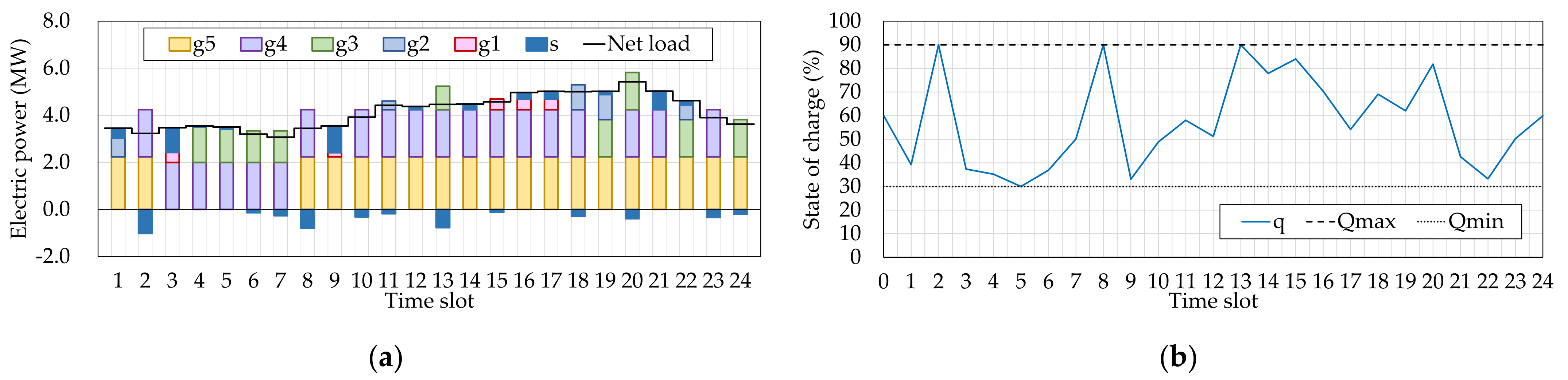
Under these conditions, the authors calculated the optimal size of the BESS while determining the optimal operation schedule (Case 1). In comparison, the operation schedules under the traditional framework of the operation scheduling were also determined. Since the BESS size is required in the traditional operation scheduling, the authors set it to 2.00 MWh (Case 2) or 3.00 MWh (Case 3) by referring to the results of Case 1 ($Q^{*}=2.62$ (MWh)). 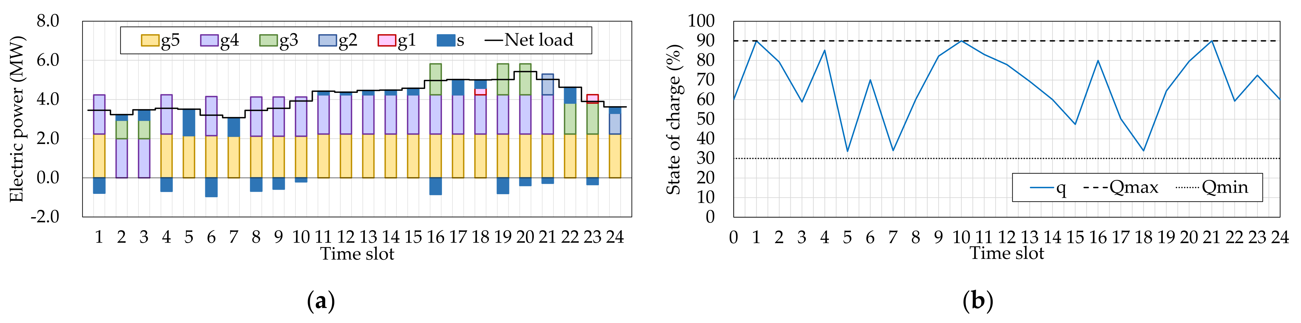Figure 4 illustrates the obtained operation schedules of Case 1, and Figure 5 and Figure 6 are the results with giving the BESS size in advance (Cases 2 and 3).

Table 2. Comparison of obtained solutions in Cases 1–3.

Case	Size of BESS	Total Cost	Investment Cost	Operational Cost
1 (Authors’ proposal)	2.62 MWh	826,930 ¥/day	14,348 ¥/day	812,582 ¥/day
2	2.00 MWh (Given)	841,753 ¥/day	10,959 ¥/day	830,795 ¥/day
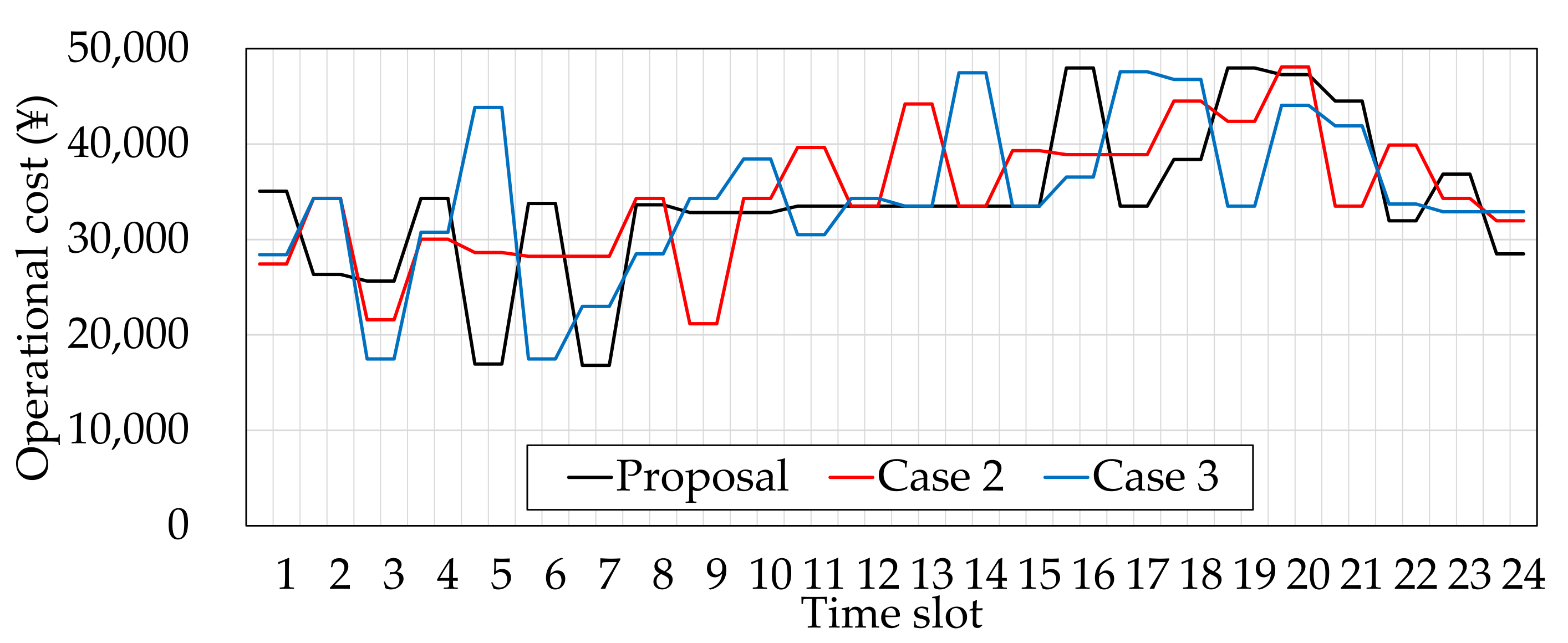
3	3.00 MWh (Given)	842,093 ¥/day	16,438 ¥/day	825,655 ¥/day

summarizes the results of their comparison, and Figure 7 displays the difference in the operational cost transitions of each case.

In all of Figure 4, Figure 5 and Figure 6, the balance of power supply and demand on the assumed net load was maintained by the coordinated operation of the CGs and the aggregated BESS. However, there were several differences in the operation schedules and their SOC levels, and they appeared as the differences between the costs, as shown in Table 2 and Figure 7. In Table 2, the operational cost in Case 1 (the authors’ proposal) was the smallest, and thus, its total cost also became the smallest. In Case 2, the investment cost was smaller than that in Case 1; however, the operational cost was increased (+2.2%). Also, the operational cost in Case 3 was larger than that in Case 1 (+1.6%), even though the largest BESS was assumed in that case. It implies a possibility that the BESS size in Case 3 was too large for the target microgrid. In the comparisons, the differences in the total costs were sufficiently small, but this is a result demonstrating that we set the BESS size in Cases 2 and 3 based on the BESS size optimized in Case 1. The differences can become large in the actual situation because we do not know the optimal BESS size. Therefore, we can conclude that the authors’ proposal is useful in the design and management of a microgrid.

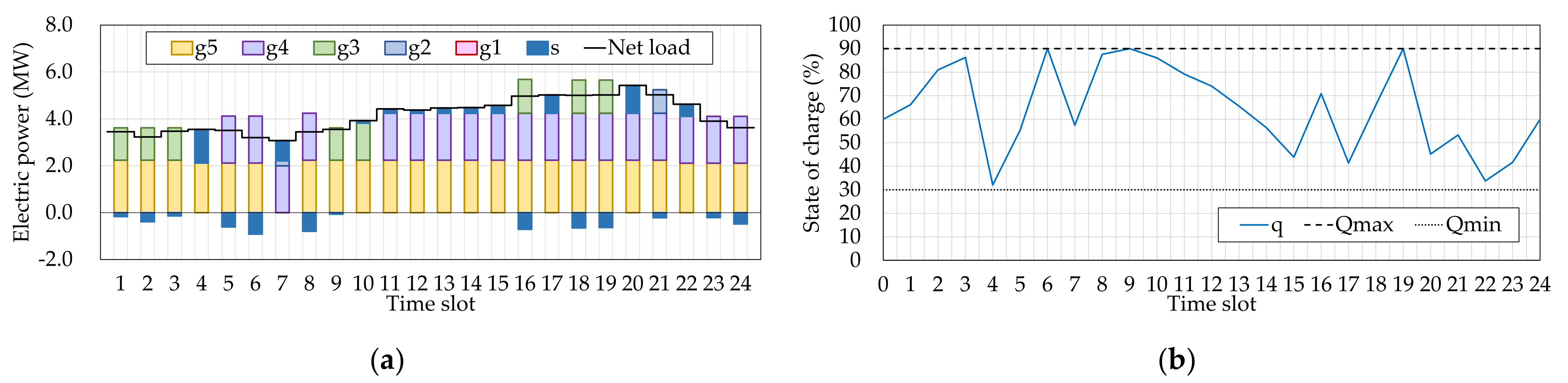
For reference, influences of the approximation strategy were evaluated through additional numerical simulations. Figure 8 displays the obtained operation schedules without the approximation strategy (Case 4).

Table 3. Comparison of obtained solutions in Cases 1 and 4.

Case	Size of BESS	Total Cost	Investment Cost	Operational Cost
1 (With approximation)	2.62 MWh	826,930 ¥/day	14,348 ¥/day	812,582 ¥/day
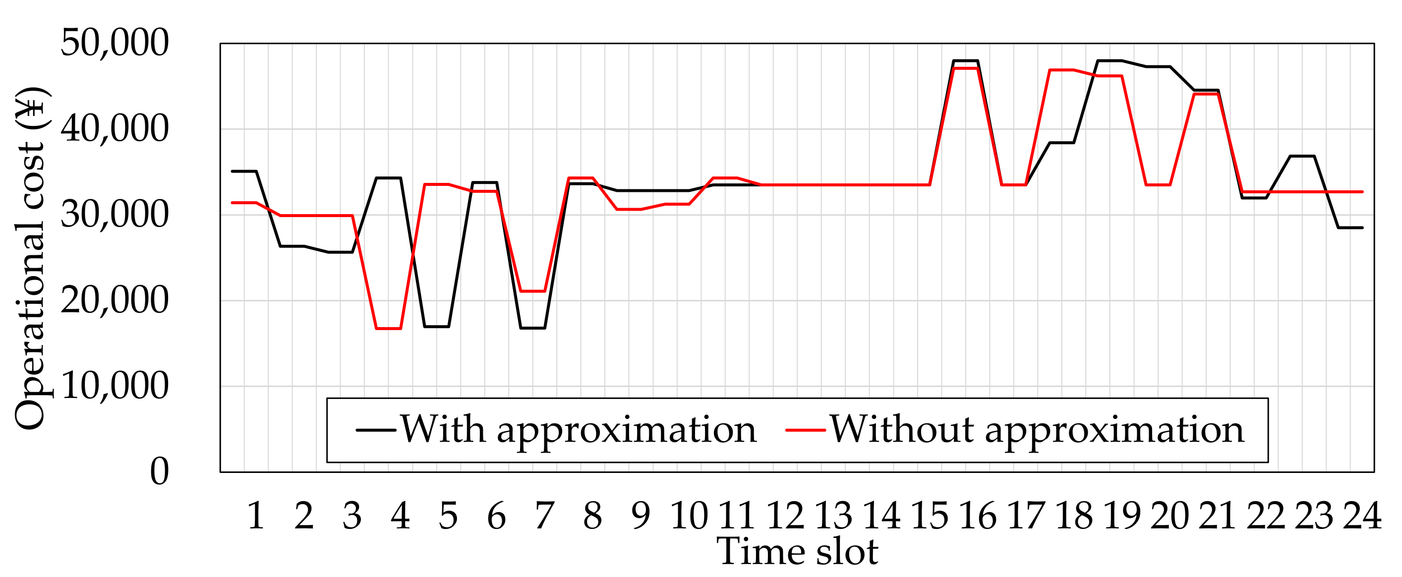
4 (Without approximation)	2.64 MWh	823,714 ¥/day	14,490 ¥/day	809,223 ¥/day

summarizes the comparison results of Cases 1 and 4, and Figure 9 illustrates the difference in their operational cost transitions. The comparison result of their computational time is shown in

Table 4. Comparison of computational time of Cases 1 and 4.

Case	Computational Time
1 (With approximation)	298 s
4 (Without approximation)	1759 s

, and the differences in the search process of the BPSO–QP are displayed in Figure 10.

These results show that the approximation strategy brought the differences in the BESS size and the operation schedules, and as a result, the total cost became slightly larger than the case without the strategy. From Figure 10, the authors concluded that the differences were originated in the search process of the BPSO–QP. In contrast, as shown in Table 4, the computational time was dramatically improved. If we treat a microgrid that has more CGs or set the target period longer, the approximation strategy becomes more effective. It can be summarized that the approximation strategy improved applicability of the BPSO–QP at the slight expense of the solution optimality.

5. Conclusions

This paper presented a problem framework and its solution method, which calculates the optimal size of BESSs, considering their cooperative operations with the other controllable components in a microgrid. In the problem formulation, the target problem was represented as a bi-level optimization to emphasize the mutual interaction in the optimal sizing and the optimal operation scheduling. However, in the solution process, the problem was treated as a type of operation scheduling problem based on the KKT approach. By the problem reformulation, the BPSO–QP, which was originally developed for the operation scheduling, became applicable. In the results of numerical simulations, the proposed framework led to better results, as compared to the case when we solved the operation scheduling problem by giving the BESS size in advance. Furthermore, it was confirmed that the approximation strategy improved the applicability of the BPSO–QP in exchange for slight deterioration in the optimality of the obtained solution.

In future works, the authors will improve the proposed solution method through discussion on appropriate selection of its basis. In addition, a method distributing the calculated BESS size into the individual BESSs will be discussed.