Investigation on Individual and Collective PV Self-Consumption for a Fifth Generation District Heating Network

Abstract

Renewable Energy Communities have been recently introduced in European legislation to promote distributed generation from renewable energy sources. In fact, they allow to produce and consume energy from shared local power plants. Low temperature district heating and cooling networks with distributed heat pumps have demonstrated their capability to exploit renewable and waste heat sources in the urban environment. Therefore, they are considered a promising infrastructure to help decarbonize the building sector. As their main operating cost is the electricity purchased by the utility for heat pumps and circulation pumps, this work investigates whether a Renewable Energy Community could help mitigate such cost by sharing electricity produced by local photovoltaic (PV) systems. The research relies on computer simulations performed with both physical and statistical models for the evaluation of electrical load profiles at the district level. Results show that due to the different seasonality between heating demand and PV production, the increase in self-consumption due to the distributed heat pumps is lower than 10%. The use of batteries does not seem convenient for the same reason. The environmental benefit of the proposed system is evident, with CO₂ emissions reduced by 72–80% compared to the current situation depending on PV power installed. It also emerged that PV sharing significantly improves the self-consumption at the district level, in particular when the installed PV power is limited (+45%). In conclusion, results suggest that current incentives on PV-sharing make Renewable Energy Communities a viable option to improve the techno-economic performance of fifth-generation district heating and cooling networks.

1. Introduction

Recently, the Renewables Energy Directive introduced a legal framework for Renewable Energy Communities (RECs), i.e., cooperative organisations for the development of local energy initiatives with non-commercial purposes. The shareholders or members of the REC may be natural persons, small medium enterprises or local authorities, including municipalities, whose primary purpose is to provide environmental, economic or social community benefits rather than financial profits [1]. According to Koirala et al. [2], Energy Communities (EC) help re-organize local energy systems to integrate distributed energy resources, engage local communities and at the same time provide useful services to the larger energy system.

As pointed out by Ceglia et al. [3], smart energy communities are essential to build a sustainable renewable energy system, which is based on a cross-sectoral approach and which seeks the optimal solution from an energy, environmental and economic point of view.

Energy communities have a key role to play in helping citizens and local authorities to invest in renewable energy and energy efficiency projects. The participation of citizens in these projects can also increase the social acceptance of such interventions at local level.

Photovoltaic (PV) systems can be installed on the roofs of public buildings or farms, as well as those of residential buildings, while biomass and biogas can be used in district heating networks [4].

Ioakimidis et al. [5] examined the supply of heating and electricity to a small Spanish village using wind turbines, a district heating system supplied by solar collectors and a biomass plant using locally-available straw for base load supply and a fossil fuel boiler for peak load, coupled with a hot water storage tank. The paper pointed out the high investment cost needed for electrical storage system as a financial barrier to the implementation of the proposed system. Bartolini et al. [6] showed that power-to-gas technologies such as fuel cells could be an economic alternative to battery systems to accommodate high shares of renewable energy production in local energy districts.

Energy Communities enable PV sharing, a practice where a single PV system supplies electricity to more than one dwelling [7]. This new regulatory framework introduces new opportunities, such as shared investments in local renewable energy projects and building refurbishments.

Garavaso et al. [8] investigated the optimal refurbishment of a multi-family building considered as an EC using the Energy Hub approach [9,10]. The study found out that remuneration on shared electricity has a great impact on the optimal refurbishment as it promotes all-electric scenarios with bigger PV installations.

In particular, for photovoltaics, the analysis carried out by Fina et al. [7] showed the benefits of energy communities in terms of higher net present value. The value added by an energy community depends on the configuration of the area (condominiums, rural area, historic centre, mixed area), the type of buildings and the number of participants.

Therefore, a later work by the same authors investigated the cost optimal allocation of shared rooftop PV capacities for neighbourhood energy communities (ECs) in rural and urban scenarios [11]. It was found that it is more advantageous for single houses in rural areas, which can benefit from the presence of diversified loads. In general, PV sharing is more advantageous when heterogeneous load profiles are present and covering the roofs with the largest available surface areas. Furthermore, the results of the analysis show that the economically optimal solution does not require all buildings to have generation facilities.

As pointed out in the survey by Fischer and Madani [12], the use of heat pumps in smart grids allows to increase grid stability, to promote the integration of renewables and to follow variable electricity prices.

Heat pumps combined with thermal and electrical storage systems can be used within Demand Side Management programs to shave peak loads of power distribution grids [13], to increase the PV self-consumption [14], or for market participation [15]. The same objectives can also be pursued at single building level with Model Predictive Control approaches [16].

In the last decade, there has been a growing interest towards low temperature district heating networks for the decarbonisation of space heating and cooling of buildings. Several projects around Europe have demonstrated that the so-called fifth generation district heating and cooling networks are able to increase the share of renewable heating and cooling in both new low-energy districts as well as in existing ones [17].

District heating networks with supply temperatures below 50 °C efficiently supply heat for space heating and domestic hot water (DHW) production to both new and old buildings through high temperature water-to-water heat pumps installed in the users’ substations. This concept is particularly interesting for urban areas where waste or renewable heat can be recovered at low costs [18]. One of these cases is Montegrotto Terme, a touristic town located in a geothermally active area in the North-East of Italy, where a large amount of groundwater is extracted from the ground, used by hotels and thermal spas, and then released to the environment. The electrical energy demand of heat pump compressors would be the highest operational cost for the operator managing the groundwater-based district heating (DH) network [18].

To the authors’ knowledge, the self-production and sharing of electricity from local renewable plants for fifth generation district heating and cooling networks has not been investigated so far.

In a preliminary paper presented at the SDEWES conference [19], the authors investigated to what extent such a thermal network could benefit from a Renewable Energy Community (REC) including all the DH customers and further inhabitants that may share the electricity produced by their PV systems.

The present study shows and discusses the gain brought by the REC with economic and environmental indicators and presents a discussion on the potential of Renewable Energy Communities for fifth generation district heating and cooling systems.

The paper is organized as follows. Section 2 presents the case study district; Section 3 the mathematical models to calculate the energy demand profiles; Section 4 reviews the assumptions, the scenarios and the performance indicators used in Section 5, where results are shown and discussed. Finally, Section 6 reviews the main conclusions.

2. Case Study

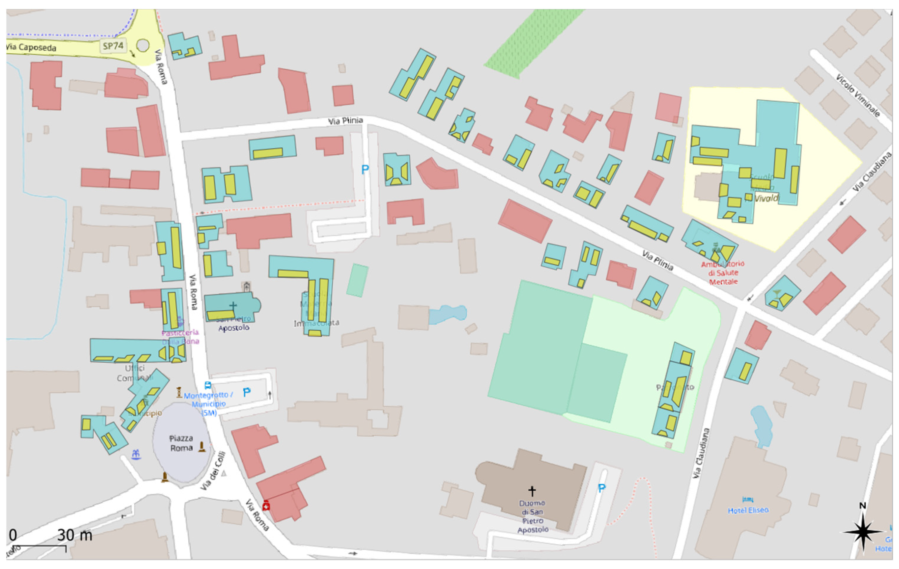
The case study district, shown in Figure 1, is a group of 61 buildings in the Municipality of Montegrotto Terme (Italy). Only 32 of them (light blue in Figure 1) were considered as potential customers for the DH network: 15 residential buildings, 10 mixed-use buildings (approximately 90 residential units and 21 commercial units) and 7 non-residential buildings (2 schools, 2 office buildings, 2 religious buildings and 1 shop). The total heated area is approximately 22,800 m². The other buildings (red footprints) are assumed to be potential members of the EC. The footprints of the buildings were sketched with QGIS [20], thus obtaining dimensions and orientations.

Each building is characterized by its main end use, age class, and number of floors. Only three age classes were considered: buildings from the ’70s (B70), ’90s (B90) and recent constructions built after 2005 (BN). Each age class corresponds to an archetype that defines the stratigraphy of the main building elements, as described in

Table 1. Building archetypes from different age classes.

Archetype	B70	B90	BN
Roof	Ceiling with reinforced brick-concrete slab (16 cm + 12 cm)	Ceiling with reinforced brick-concrete slab (24 cm)	Ceiling with reinforced brick-concrete slab, insulated (24 cm + 10 cm)
U [W/(m2 K)]	1.34	0.79	0.33
Ground Floor	Floor with reinforced concrete slab, traditional screed (12 cm)	Floor with reinforced concrete slab, lightweight screed (12 cm)	Floor with reinforced concrete slab, lightweight screed (12 cm), insulation (10 cm)
U [W/(m2 K)]	1.42	0.90	0.23
Internal Ceiling	Brick-concrete slab, traditional screed (16 cm + 10 cm)	Internal Floor with reinforced brick-concrete slab (24 cm), trad. screed (12 cm), insulation (2 cm)	Brick-concrete slab, lightweight screed (12 cm), insulation (10 cm)
U [W/(m2 K)]	1.27	1.22	0.52
External Wall	Hollow/solid bricks with cavity (12-8-12)	Hollow/solid bricks with insulated cavity (25-4-8)	Perforated bricks and medium insulation (30-10)
U [W/(m2 K)]	0.98	0.60	0.30
Internal Wall	Hollow tiles and plaster (8 cm)	Hollow tiles and plaster (8 cm)	Hollow tiles and plaster (8 cm)
U [W/(m2 K)]	2.39	2.39	2.39
Window	Double glazing, air filled, metal frame without thermal break	Double glazing, air filled, air filled, metal frame with thermal break	Low-e double glazing, air/gas filled, wood frame
U [W/(m2 K)]	3.7	3.4	2.2
g-value	0.7	0.7	0.27
τv	0.79	0.79	0.64

. The internal loads were defined according to the main end-use of the building considered: either office, school or residential. Each category was given a different schedule for electric loads (appliances and illumination), occupancy, setpoint temperature of the indoor air and relative humidity and ventilation rates according to Annex C of EN 16798-1 Standard [21]. In particular, for the heating period (from 15 October to 15 April) the setpoint of temperature was set to 20 °C and for cooling period (from 15 June to 15 September) to 26 °C. In residential buildings the heating/cooling system is always on, whereas in offices it is active from 8 a.m. to 6 p.m. during working days only. In schools, it is on from 6 a.m. to 5 p.m.; a pre-heating of three hours was set to avoid excessive peak loads. It was assumed that there is only natural ventilation with a nominal air change rate of 1.5 volumes/hour during the operating time, to avoid an overestimation of the heat load.

Table 2. Assumptions for the internal heat gains, ventilation and infiltration losses.

		Residential	Office	School
Occupancy	[W/m2]	2.83	4.7	13.8
Appliances	[W/m2]	3	12	8
Lights	[W/m2]	3	12	8
Infiltration	[vol/h]	0.2	0.2	0.2
Humidity	[g/(m2 s)]	2.12	3.53	11.1
Ventilation	[m3/(s m2)]	1.8	2.88	1.5 vol/h

shows the nominal values.

3. Models

An Urban Building Energy Model called EUReCA was applied to the case study described above and the output was the hourly heating/cooling power for every building. To obtain the final energy for heating, the hourly net energy was divided by an average global efficiency. This was obtained considering the emission, regulation end distribution efficiency from UNI/TS 11300-2 Standard [22]. The average global efficiency was equal to 84%. The heat pumps were sized for every building connected to the low temperature district heating network. The design power was assumed equal to the peak load for residential users and to the power corresponding to 98% of heating demand on the load duration curve for users with discontinuous operation. A steady-state model of water-to-water heat pumps was then used to calculate the corresponding electrical profiles for heating and cooling. Such physics-based models were used together with stochastic profile generators for DHW and electrical consumption.

3.1. Thermal Load Profiles for Space Heating

The EUReCA [23] is based on a lumped-capacitance model that combines all the building components considering their thermal properties to obtain a discrete number of parameters to reproduce building thermal behaviour.

The model proposed by the Standard VDI 6007-1 [24] is based on seven thermal resistances and two capacitances, as shown in F. The two capacitances allow to simulate the transient behaviours of adiabatic (IW) and non-adiabatic (AW) building components. This is important because structures under asymmetrical loads behave differently compared to adiabatic building components. The parameters R_1;AW and R_1;IW, C_1;AW and C_1;IW are the dynamic thermal resistances and capacitances of non-adiabatic and adiabatic components, respectively. The combination of different building components to achieve equivalent thermal resistances and capacitances is obtained by parallel connection of complex thermal resistances, as explained in the Standard [24]. R_ges,AW is the overall thermal resistance of the non-adiabatic building components and R_ve is the thermal resistance due to ventilation that connects the internal air temperature θ_i with the node of the supply air temperature θ_sup.

The model assumes that all building surfaces contribute to the radiation exchange proportionally to their respective surface areas. The effects of solar radiation absorbed by the external walls and the radiation emitted by the external surfaces to the external environment (sky and ground) are included in the equivalent air temperature θ_A;eq;gew. The equivalent outdoor temperature of each exterior surface is calculated as follows:

$${\theta }_{e,eq}={\theta }_e+\mathsf{\Delta }{\theta }_{e,eq,lw}+\mathsf{\Delta }{\theta }_{e,eq,sw}$$

(1)

where ∆θ_e;eq;lw is the temperature drop due to the thermal radiation emitted by external surfaces to the sky and to the ground and ∆θ_e;eq;sw is the temperature gain due to the solar energy absorbed by opaque walls. Radiative and convective heat gains (including the heating/cooling load) are divided between three different nodes: the indoor air temperature θ_i, the surface temperature of internal and external walls θ_s;IW and θ_s;AW. The thermal balance on the five nodes of the equivalent electrical circuit shown in Figure 2 leads to a linear system of five equations. The latter can be solved for each timestep fixing the internal temperature to a set-point and calculating the heat load ${\Phi }_{hc}$. The model presented includes the calculation of the solar position and incidence angle for vertical surfaces according to the orientation of the walls with the formula provided by Duffie and Beckman [25]. The full calculation procedure of the solar heat gains has been described in Zarrella et al. [23,26] and is not repeated here for sake of brevity.

3.2. Thermal Load Profiles for DHW Consumption

The domestic hot water profiles were considered only for residential buildings and they were obtained using the software DHWCalc [27] assuming standard probability distribution functions and an average daily consumption of 150 L/unit. The resulting stochastic profiles of hot water draw-offs consumed was converted into thermal energy, considering an increase of temperature from 10 to 40 °C. The electric consumption of heat pumps was calculated considering a constant COP equal to 3.5.

3.3. Electric Load Profiles of the Heat Pumps

The model for the water-to-water heat pumps has been already described in Vivian et al. [18]. The simplified model uses polynomial functions of the evaporating and condensing temperatures to calculate the electric power consumed by compressors $W_{el,hp}$ and the heat flow rate at the evaporator $Q_{ev}$, as reported in Equations (2) and (3), respectively.

$$W_{el,hp}=a_0+a_1{\theta }_{ev}+a_2{\theta }_{cd}+a_3{\theta }_{ev}^2+a_4{\theta }_{ev}{\theta }_{cd}+a_5{\theta }_{cd}^2+a_6{\theta }_{ev}^3+a_7{\theta }_{ev}^2{\theta }_{cd}+a_8{\theta }_{ev}{\theta }_{cd}^2+a_9{\theta }_{cd}^3$$

(2)

$$Q_{ev}=b_0+b_1{\theta }_{ev}+b_2{\theta }_{cd}+b_3{\theta }_{ev}^2+b_4{\theta }_{ev}{\theta }_{cd}+b_5{\theta }_{cd}^2+b_6{\theta }_{ev}^3+b_7{\theta }_{ev}^2{\theta }_{cd}+b_8{\theta }_{ev}{\theta }_{cd}^2+b_9{\theta }_{cd}^3$$

(3)

The coefficients a_i and b_i depend on the compressor and are usually given by the manufacturers. The evaporating temperature ${\theta }_{ev}$ depends on the network temperature, whereas the condensing temperature ${\theta }_{cd}$ depends on the supply temperature for the heating system of the building, which in turn depends on the external temperature and type of building. Finally, the heat flow rate supplied by the heat pump condenser is equal to:

$$Q_{cd}=Q_{ev}+{\eta }_{el,comp}{W}_{el,hp}$$

(4)

where ${\eta }_{el,comp}$ is the efficiency of the compressor engine, fixed to 95%. The coefficient of performance COP was defined as the ratio between the heat flow rate at the condenser and the electric power required by the compressor engine.

3.4. Electric Load Profiles for Other Uses

The electric load profiles for other uses of residential buildings were evaluated using the Flexmeter load profile generator [28]. This model simulates stochastic power profiles for users with pre-selected sets of appliances. It considers the appliances owned by each customer, its average energy consumption during the year, the overall annual energy consumption for each customer and the standard load profile available at aggregated level. The model combines the advantages of bottom-up and top-down approaches. In fact, it uses a bottom-up approach to generate the random profile from the aggregation of single appliances like the one in Figure 3a, but the allocation of events is driven by the aggregated standard load profiles like the one in Figure 3b. The higher the average power use is during the day, the higher is the probability of there being a specific device active in that moment. In this way, the model can be used to generate representative data of a realistic scenario both at grid level and at single building level. The input data are the standard load profiles, the appliances profiles, statistical data about the diffusion and percentage of energy consumption of different appliances. The scenarios generation consists in determining the set of appliances owned by each user and the level of consumption associated with each device. It is possible to add a level of randomness to take in account different levels of efficiency. The standard electric load profiles for residential buildings were based on the aggregated profiles of ATLANTIDE project [29]. The annual consumption was fixed to 2500 kWh, with a randomness of 10% from data of ARERA [30].

The number of electric profiles is equal to the number of housing units. The latter was known for some buildings and was guessed for some other by assuming an average gross unit area of 120 m², thus obtaining 90 residential units. As far as mixed-use buildings were concerned, their electric load profiles were taken from ATLANTIDE database for offices and shops inside condominiums (21 units, 70% office and 30% commercial). The annual electric consumption was set at 3000 kWh. As regards non-residential buildings, the normalized profiles were taken from EN 16798-1 Standard [21] and calibrated using real consumption data available from the electric energy bills. Further details on these assumptions can be found in the previous paper [19].

3.5. Photovoltaic Systems

The electric production of photovoltaic (PV) systems was calculated with a model based on PVGIS [31]. The inputs to the model are the weather data (direct and diffuse solar radiation on the horizontal surface, external dry bulb temperature and wind speed) and the information of the PV module: position, surface area, orientation and tilt angle as well as its nominal efficiency. The total radiation on the module plane is calculated estimating the beam solar radiation, the diffuse solar radiation with isotropic sky hypothesis and the reflected solar radiation with an albedo coefficient -set to 0.2. The incident angle of beam solar radiation is calculated from the position of the sun and of the PV plane. The performance of the module is evaluated as a function of air temperature, incident solar radiation and wind speed with the same procedure explained in Zarrella et al. [26].

4. Methods

From a thermodynamic point of view, the electrical energy of PV systems is more valuable due to its high exergy content and should be used directly as work for mobility, industry etc, while heating and cooling could be satisfied with the production of heat from other sources like solar thermal collectors and waste heat. The exergy imbalance of the proposed system has not been considered in this paper, giving priority to electric heat pumps that show greater flexibility of operation and whose diffusion is expected to increase in the coming years.

4.1. Main Assumptions for District Simulations

The evaporation temperature in the heat pumps was considered constant and equal to 27 °C, considering a network temperature of 40 °C, a difference of temperature from supply and return of 10 °C and a minimum difference of temperature between the two fluids of 3 °C.

The study assumed the same supply temperature curves adopted in a previous analysis [18]. For the cooling season, only the sensible loads were considered, and they were converted to electric consumption, considering air-to-air systems with a constant COP equal to 3.2. The cooling systems were considered only for the buildings connected at the DH. The photovoltaic systems were designed using the software QGIS [20], identifying all the available surfaces on the roofs of buildings, using the satellite images, except for north-oriented surfaces –see Figure 1. Every surface was assigned the azimuth angle and the tilt angle. The nominal efficiency of the modules was set to 15%. The total available area on the considered buildings was around 2815 m², that correspond to 422 kW of peak power. The assumptions concerning costs have been summarised in

Table 3. Summary of economic assumptions.

Energy Vector	Variable		Unit	Value
Natural gas	${\eta }_{gb}$	Gas boiler efficiency	%	90
	$e_{gb}$	Gas boiler CO2 emission [32]	kg/kWh	0.202
	$p_{gb}$	Gas price	€/kWh	0.085
Electricity	$e_{el}$	Electricity CO2 emission [33]	kg/kWh	0.290
	$p_{el}^{\left(du\right)}$	Electricity price for domestic users	€/kWh	0.22
	$p_{el}^{\left(dho\right)}$	Electricity price for district heating operator	€/kWh	0.17
	$p_{el,sell}$	Sell electricity price	€/kWh	0.05
	$p_{el,shared}$	Shared electricity tariff	€/kWh	0.168
Heat	$p_{dh}$	District heat tariff	€/kWh	0.10
-	$I_{dh}$	DH Investment cost	€	1,000,000
-	$I_{hp}$	HP Investment cost	€/kW	350
-	$I_{pv}$	PV Investment cost	€/kW	1500

, where there is a different electricity price between domestic users and district heating operator. The shared electricity tariff includes the selling price and an incentive set forth in current legislation.

The energy consumption calculated with the models described in the previous section could not be verified against measured data. However, the actual gas consumption was available for seven non-residential buildings. The difference between actual and calculated values varied considerably from building to building (between −46 and +97%, with an average of +22% for simulated thermal energy demand). This difference depends mainly on the uncertainty about their actual use. For three public buildings, the actual electrical consumption was also available from the bills. It was found that the models significantly overestimate the consumption. Therefore, the corresponding profiles were scaled down using a multiplier (0.34).

4.2. Simulated Scenarios

The simulated Renewable Energy Community include both district heating customers and buildings in the surrounding area, as explained in the previous Section. Four different scenarios arise from the combination of EC members and installed PV capacity, as reported in

Table 4. Summary of the simulated scenarios.

Scenario	S1	S2	S3	S4
Buildings in the REC	32	32	61	61
PV plants (-)	32	9	32	9
PV power (kW)	422	200	422	200

. In scenarios S2 and S4, the photovoltaic power was limited at 200 kW, which is the current limit set by the Italian legislation. PV systems were placed on the roofs with the largest area, which seems to be a convenient choice when the PV capacity is limited [11].

In one scenario, a centralised electric storage was also introduced using a simplified one-node model, with the purpose of evaluating the increase of self-consumption in the REC. Different size of storage were simulated with increments of 100 kWh up to a maximum of 500 kWh. In this model, the level of charge of batteries was calculated every hour, stating from zero and incrementing or reducing by the quantity of electric energy that exceeds or lacks at the consumption of the entire community, until it reaches the maximum or zero. In this model, the efficiency of charge and discharge and the depth of discharge were not taken into account.

4.3. Economic and Environmental Indicators

The electricity consumed by the i-th building $W_{el,dem}^{\left(i\right)}$ is equal to the sum between the electricity required by the heat pumps (if present) and the electricity consumed for other uses:

$$W_{el,dem}^{\left(i\right)}=W_{el,hp}^{\left(i\right)}+W_{el,ou}^{\left(i\right)}$$

(5)

The electric self-consumption of the i-th building corresponds to the minimum, in every hour, between the electricity produced and the electricity consumed:

$$W_{el,self}^{\left(i\right)}=\left(W_{el,dem}^{\left(i\right)},W_{el,pv}^{\left(i\right)}\right)$$

(6)

In the case of a building with more housing units the energy consumed is the sum of the energy consumed by each unit. The collective self-consumption of REC was evaluated as the minimum, in every hour, between the energy fed into the grid from photovoltaic systems and the electrical demand of REC members:

$$W_{el,self}^{REC}=\left({\displaystyle \sum }_{iϵR}^{}{W}_{el,dem}^{\left(i\right)},{\displaystyle \sum }_{iϵR}^{}{W}_{el,pv}^{\left(i\right)}\right)$$

(7)

where R represents the set of REC members. For simplicity, all users of the same building were considered participating to the REC. The shared energy is considered as the difference between the collective self-consumption and the sum of the single self-consumption of the buildings:

$$W_{el,shared}^{REC}=W_{el,self}^{REC}-{\displaystyle \sum }_{iϵR}^{}{W}_{el,self}^{\left(i\right)}$$

(8)

The cost associated to electricity consumption depends on the amount of shared energy as shown in Equation (9), where the price of energy bought from the grid depends on the type of customer:

$$C_{el}=\left(p_{el}^{\left(du\right)}{W}_{el,dem}^{\left(du\right)}+p_{el}^{\left(dho\right)}{W}_{el,dem}^{\left(dho\right)}\right)-p_{el,shared}{W}_{el,shared}^{REC}-p_{el,sell}{W}_{el,sell}$$

(9)

where $W_{el,sell}$ is the electricity sold to the grid. The simple payback time of DH network and HPs is the ratio between the investment cost and the profit:

$$PB{T}_{dh}=\frac{I_{dh}+I_{hp}{P}_{hp}}{p_{dh}{Q}_{dh}-p_{el}^{\left(nres\right)}{W}_{el,hp}}$$

(10)

where $P_{hp}$ is the HPs power installed, $Q_{dh}$ is the heat sell to the customers and $W_{el,hp}$ is the electricity consumed by the heat pumps. The simple payback time of PV systems depends on the cost of electricity:

$$PB{T}_{pv}=\frac{I_{pv}{P}_{pv}}{p_{el,sell}{W}_{el,sell}+p_{el,shared}{W}_{el,shared}^{REC}}$$

(11)

where $P_{pv}$ is the photovoltaic power installed. Finally, the reduction of CO₂ emissions was calculated compared to the current situation without the district heating and the PV systems:

$$\mathsf{\Delta }e=Q_{gb}{e}_{gb}+W_{el,pv}{e}_{el}-W_{el,ph}{e}_{el}$$

(12)

5. Results and Discussion

Authors should discuss the results and how they can be interpreted from the perspective of previous studies and of the working hypotheses. The findings and their implications should be discussed in the broadest context possible. Future research directions may also be highlighted.

5.1. Simulation Results

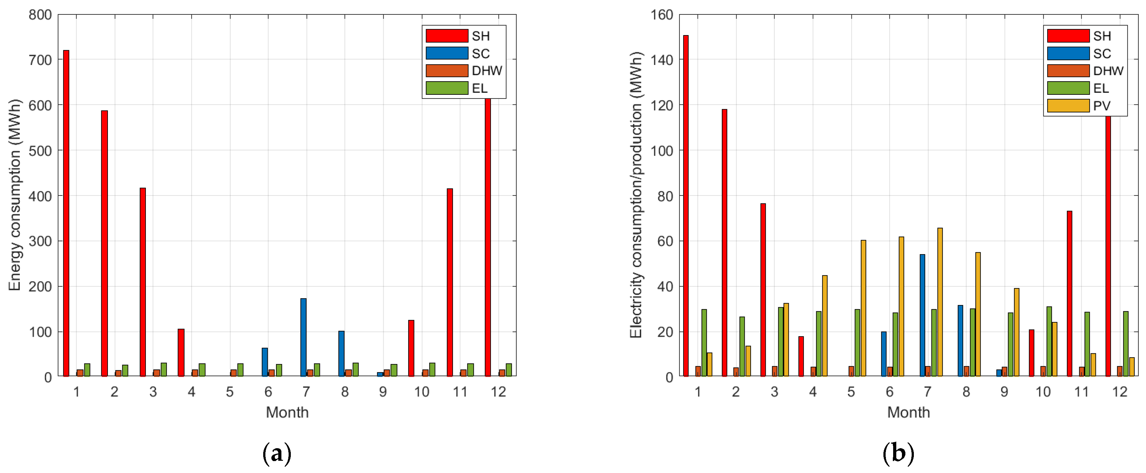
From the simulations, the thermal energy for space heating is equal to 3015 MWh per year, 187 MWh for DHW production and 348 MWh for space cooling. The electric consumption of HP is 586 MWh for heating, 53 MWh for DHW and 109 MWh for cooling. The electric consumption for other uses is 350 MWh per year and the PV production is 426 MWh with 422 kW installed or 203 MWh with 200 kW installed. The monthly profile of thermal energy end-use and the corresponding electricity needs is reported in Figure 4 for scenario S1.

It can be seen that in the winter months, the energy requirements for heat pumps were considerably higher than other electrical consumption and photovoltaic production. While in summer months, renewable electricity production exceeded the electrical needs of buildings. In this scenario, an energy community that also involves users without heat pumps seems useful to take full advantage of the energy produced in the summer months. This is even more relevant for buildings with high roof areas but low summer loads, such as schools or other buildings without summer cooling systems.

The previous considerations rely on monthly energy needs. However, matching local electricity supply and demand clearly depends on their simultaneity, that must be analysed on a finer temporal resolution.

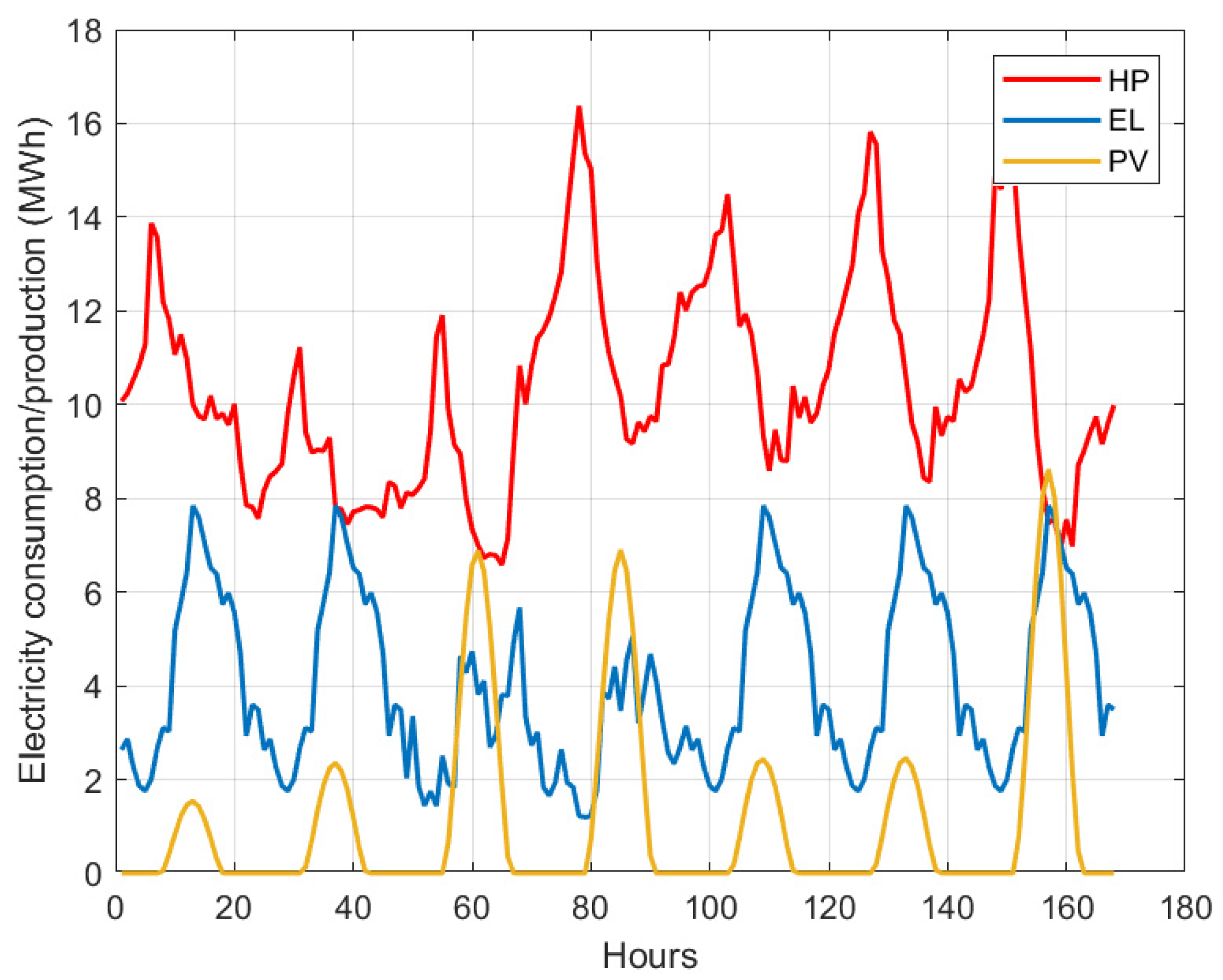
Figure 5 shows hourly trends due to heat pump (HP) and other electrical devices (EL) for one week in March for a mixed-use building with three commercial units and ten residential units with low thermal insulation. In addition, the Figure includes the hourly photovoltaic production (PV) for a 20.8 kW system, as assumed for this building based on the available roof area, has been reported. It can be observed that the electrical load of the heat pump is high but discontinuous, as it is influenced by the high fluctuation in the external air temperature between day and night. In this example, the local electrical production is not sufficient to cover the electrical loads but contributes in any case to reduce the withdrawals from the grid.

5.2. Self-Consumption and Energy Sharing in the Considered Scenarios

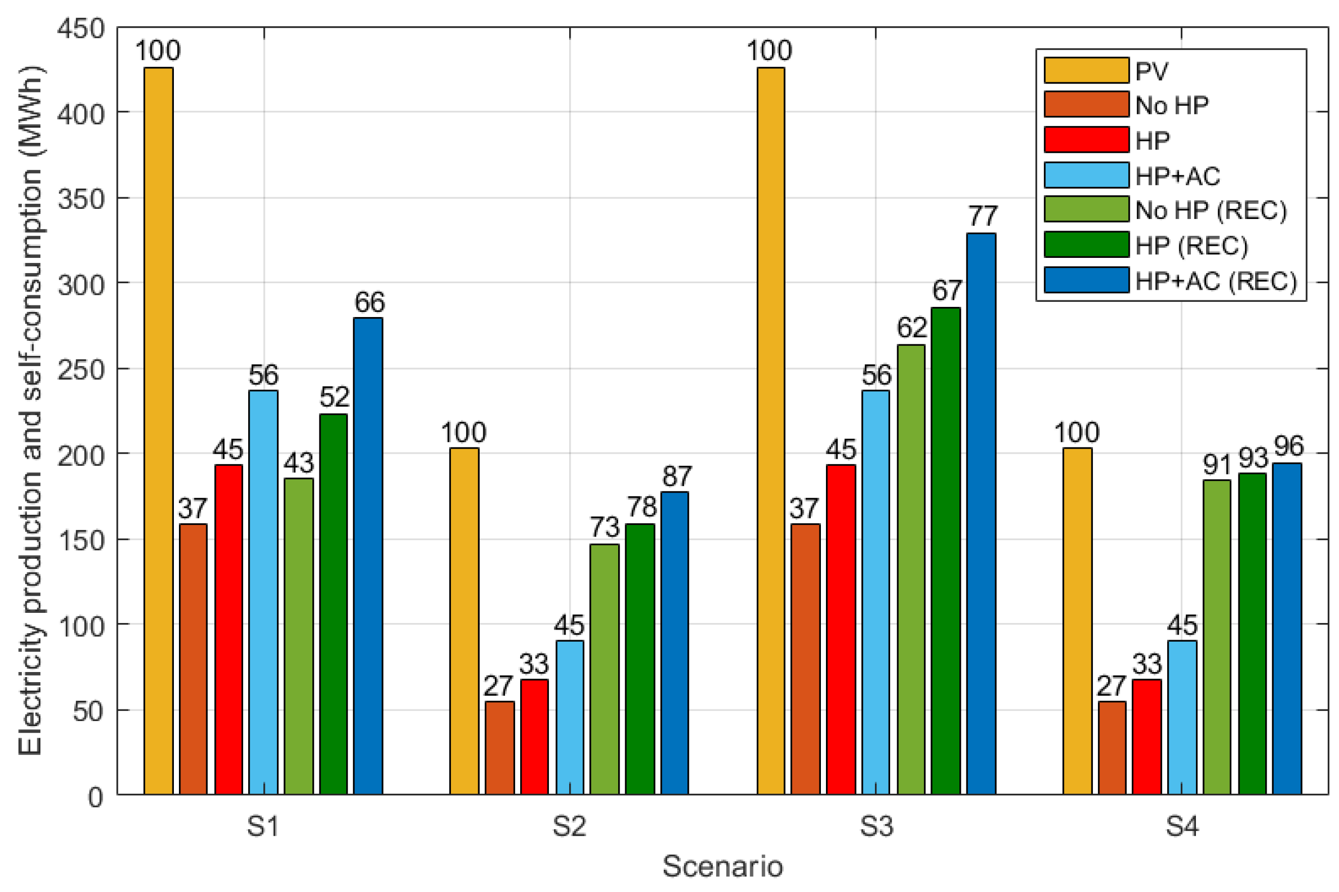
In Figure 6, the PV production and the levels of self-consumption are reported for the different scenarios considered. It can be noticed that the self-consumption increases from 5–9% with the introduction of HP for heating and DHW, this limit is caused by the different seasonality of PV production and HP consumption, the first is higher in summer, the second in winter, so there is not a good match between them. With the introduction of a REC, the self-consumption increases by 6–7% in S1 and by 45–46 % in S2. This important difference is caused by the fact that in the first scenario all the buildings have their own PV system, so the advantage of shared electricity is little, whereas in the second scenario only few buildings have the PV systems. In such cases, the REC allows a dramatic increase in the amount of electricity shared by different buildings.

If the Energy Community is enlarged to other users without HP (61 buildings with a total demand of electricity equal to 599 MWh/year), the self-consumption increases by 22–25% in scenario S3 and by 60–64% in scenario S4 with respect to the case without the REC. On the other hand, in this case the benefit of HP is reduced (2–5%). Adding the cooling load, the self-consumption increases by 11% without REC, and by 14% with REC in scenario S1, and by 12% without REC, and by 9% with REC in scenario S2. So, the benefit of cooling loads is more relevant if the PV installed is higher, both with and without REC. With more users in the Community, the advantage of cooling is limited: only 4% in scenario S3 and by 6% in S4. This happens because the higher the self-consumption, the less the additional cooling loads contribute to increasing it.

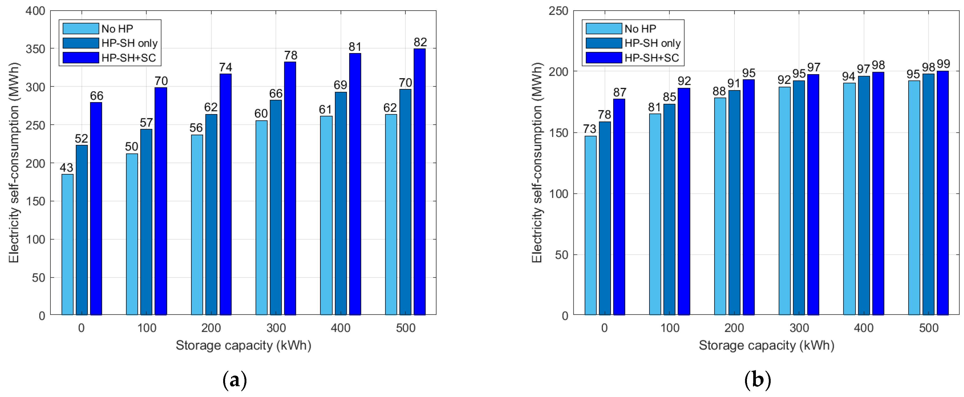
The electric self-consumption with electrical storage system is reported in Figure 7 for different storage capacities. Under scenario S1—see Figure 7a—the self-consumption increases from 43 to 62% without HPs, from 52 to 70% with HPs and from 65 to 82% including the cooling systems. It is possible to observe that the self-consumption reaches an upper limit. The latter is because the electrical energy can be stored daily, which poses no remedy on the seasonal mismatch between power demand and supply. If the PV power installed is low as in Scenario S2, the self-consumption can reach values near 100%—see Figure 7b. In the latter case, the advantage of additional heating and cooling loads are rather limited.

5.3. Economic and Environmental Indicators

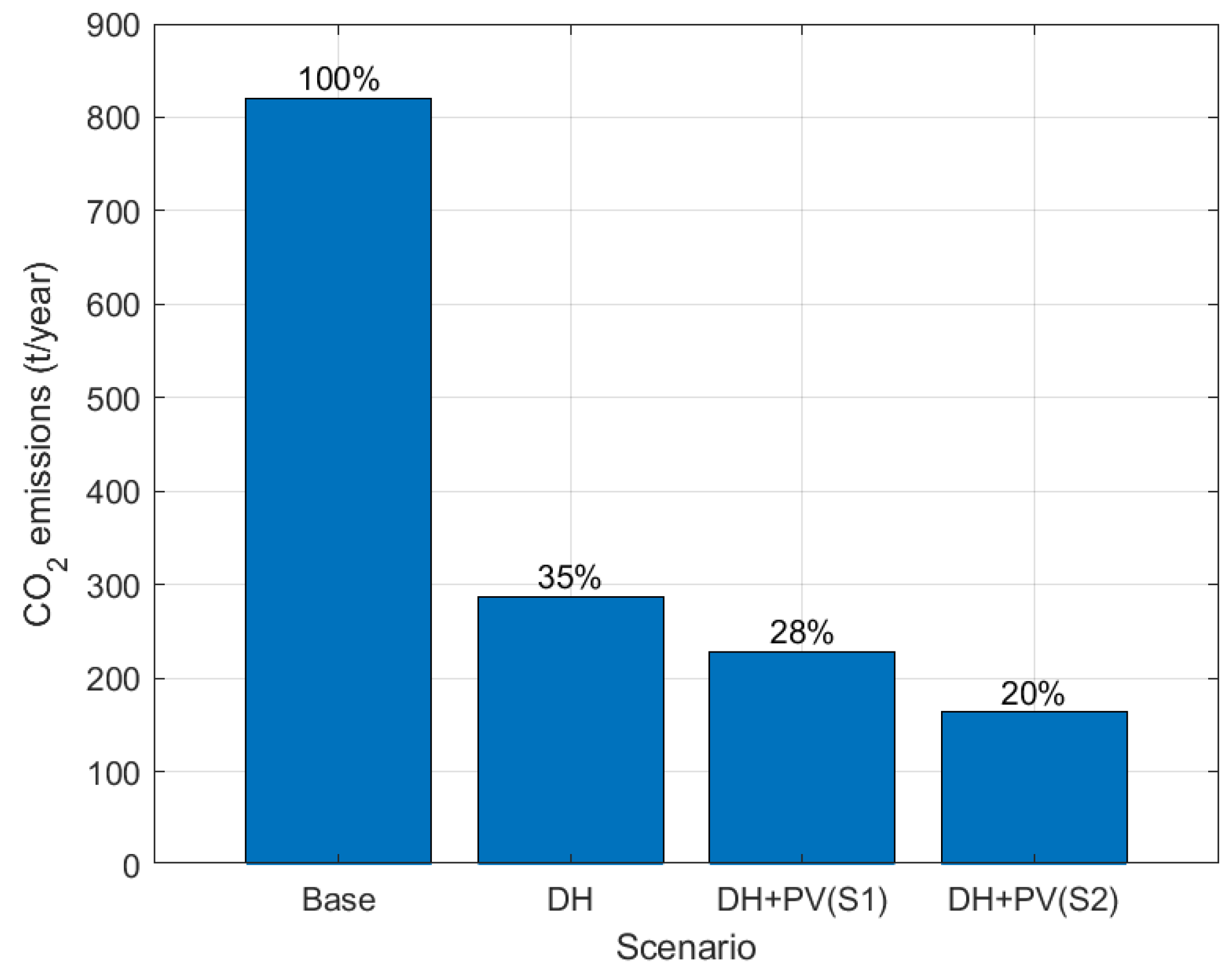
The CO₂ emissions corresponding to the initial situation without the district heating network are reported in Figure 8, including cases with the DH only and with both DH and PV systems. With the district heating system, the reduction of emissions $\mathsf{\Delta }e$ is 65%. The reduction reaches 72% and 80% with 200 kW and 422 kW of PV installed, respectively. Emissions are therefore reduced to one third of the initial ones by using a low-temperature waste heat source, and to one fifth by adding photovoltaics. Considering that most of the buildings are old, a refurbishment of some of them would lead to a further reduction in consumption.

Finally, a simple analysis has been conducted to investigate whether the investment in the PV systems pays off from the perspective of the whole Energy Community and from the perspective of the DH utility.

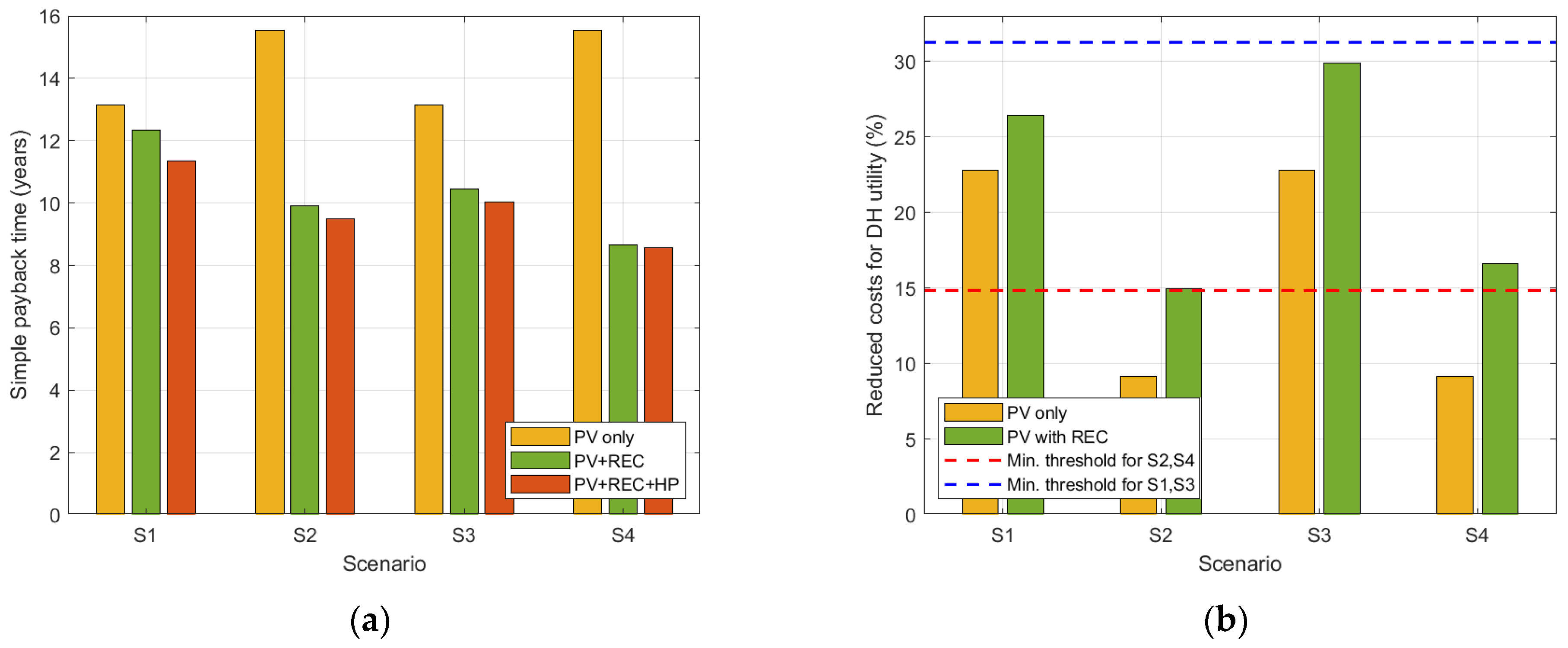
To this end, the simple payback time for PV systems is reported in Figure 9a, where cooling systems are not considered. The presence of a REC reduces the payback time in all the scenarios due to the incentive on shared electricity. The advantage is more relevant in S2 and S4, because in this case the installed PV power was limited and the shared electricity level was rather high. It can be observed that the presence of HPs reduced the simple payback time, but not as significantly (1.4 to 8.1%) if only SH and DHW were included in the analysis.

Figure 9b shows the reduction in operating costs for the DH utility linked to the local self-production of electricity. The investment in the PV system pays off only when such reduction equals the investment increase for the DH utility, shown by the red and blue dashed lines for the lower and upper PV power installed. This Figure must be interpreted as a worst-case scenario because the low temperature network does not provide space cooling.

It can be observed that investing in PV systems does not lead to a corresponding reduction in operating costs without REC. The latter helps cutting electricity supply costs by 3.6 to 7.4%. Despite such significant improvement, only S2 and S4 scenarios lead to a benefit similar to or greater than the investment, confirming that the correct sizing of the overall PV power is crucial for a cost-optimal sector coupling.

6. Conclusions

This paper analyses the mutual benefits between a low temperature thermal grid with booster heat pumps and a Renewable Energy Community (RECs) based on a shared PV production.

The hypothesis is that self-producing and sharing electricity with distributed rooftop PV-systems would help the utility make fifth-generation district heating and cooling networks more economically convenient and, at the same time, an increase in the electrical demand due to booster heat pumps would be beneficial for the REC members.

To this end, four scenarios were investigated arising from the combination of two levels of nominal PV power and two levels of participation to the REC in an Italian town where a low temperature district heating network is currently under evaluation by the municipal administration. Such a network would be entirely supplied by renewable wastewater at around 40 °C.

The study found out that the benefit brought by the heat pumps to the REC is rather limited due to a seasonal mismatch between summer PV production and winter heating demand. In fact, computer simulations showed that the increase of shared electricity linked to the district heating heat pumps is limited to +9% in the best case.

In the other direction, the possibility to cut operational costs for the DH utility seems to be more attractive because of the incentives put in place for the energy shared among REC members by current Italian legislation.

Results show that the benefit brought by REC depends on the size and number of PV systems installed: there seems to be an optimal aggregated size of installed PV systems that maximizes the collective PV self-consumption.

If the REC includes other users beside those connected to the DH network, the PV self-consumption of the whole community may reach 90% but the relative contribution of the heat pumps is reduced. How to share this benefit between district-heated and other REC members depends on the business model adopted.

In conclusion, the research found out that a PV-based REC could help reduce operational costs for district heating systems with a high number of heat pumps.

These findings lay the groundwork for a possible technical-economic optimization of the system and leaves room for possible innovative business models for the combined sale of heat and energy. Future research could therefore look at the optimal design of Renewable Energy Communities based on multiple PV systems in different electrical demand scenarios. The results that may emerge from such research would be of interest not only to the scientific community, but also to energy service companies and engineering companies that commercialize and/or design renewable energy projects for local communities. In addition, the increasing electrification of the heating and cooling sector and the possibility to produce and share electricity locally need to be further analysed, as they could give rise to new business models based on selling electricity, heat and cooling as a single energy asset. These possibilities need to be supported by an appropriate regulatory framework.

The main limitations of the present study are, on the modelling side, ignoring latent cooling loads during summer and assuming buildings as the smallest consumption units instead of individual apartments. The first assumption leads to an underestimation of self-consumption in summer, while the latter affects the energy sharing figures. In addition, more electricity uses could be considered, such as electric vehicles charging.

References

1. Roberts, J.; Frieden, D.; d’Herbemont, S. Report from the COMPILE project (H2020-824424). Energy Community Definitions. Available online: https://www.compile-project.eu/wp-content/uploads/Explanatory-note-on-energy-community-definitions.pdf (accessed on 10 December 2021).
2. Koirala, B.P.; Koliou, E.; Friege, J.; Hakvoort, R.A.; Herder, P.M. Energetic Communities for Community Energy: A Review of Key Issues and Trends Shaping Integrated Community Energy Systems. Renew. Sustain. Energy Rev. 2016, 56, 722–744. [Google Scholar] [CrossRef] [Green Version]
3. Ceglia, F.; Esposito, P.; Marrasso, E.; Sasso, M. From Smart Energy Community to Smart Energy Municipalities: Literature Review, Agendas and Pathways. J. Cleaner Production 2020, 254, 120118. [Google Scholar] [CrossRef]
4. Caramizaru, A.; Uihlein, A.; European Commission; Joint Research Centre. Energy Communities: An Overview of Energy and Social Innovation; Publications Office: Luxembourg, 2020; ISBN 978-92-76-10713-2. Available online: https://data.europa.eu/doi/10.2760/180576 (accessed on 10 December 2021).
5. Ioakimidis, C.; Koutra, S.; Bagheri, A.; Genikomsakis, K. Solar Thermal and Wind Energy Applications: Case Study of a Small Spanish Village. Therm. Sci. 2018, 22, 2163–2176. [Google Scholar] [CrossRef] [Green Version]
6. Bartolini, A.; Carducci, F.; Muñoz, C.B.; Comodi, G. Energy Storage and Multi Energy Systems in Local Energy Communities with High Renewable Energy Penetration. Renew. Energy 2020, 159, 595–609. [Google Scholar] [CrossRef]
7. Fina, B.; Auer, H.; Friedl, W. Profitability of PV Sharing in Energy Communities: Use Cases for Different Settlement Patterns. Energy 2019, 189, 116148. [Google Scholar] [CrossRef]
8. Garavaso, P.; Bignucolo, F.; Vivian, J.; Alessio, G.; De Carli, M. Optimal Planning and Operation of a Residential Energy Community under Shared Electricity Incentives. Energies 2021, 14, 2045. [Google Scholar] [CrossRef]
9. Geidl, M.; Koeppel, G.; Favre-Perrod, P.; Klockl, B.; Andersson, G.; Frohlich, K. Energy Hubs for the Future. IEEE Power Energy Mag. 2007, 5, 24–30. [Google Scholar] [CrossRef]
10. Wu, R.; Mavromatidis, G.; Orehounig, K.; Carmeliet, J. Multiobjective Optimisation of Energy Systems and Building Envelope Retrofit in a Residential Community. Appl. Energy 2017, 190, 634–649. [Google Scholar] [CrossRef]
11. Fina, B.; Auer, H.; Friedl, W. Cost-Optimal Economic Potential of Shared Rooftop PV in Energy Communities: Evidence from Austria. Renew. Energy 2020, 152, 217–228. [Google Scholar] [CrossRef]
12. Fischer, D.; Madani, H. On Heat Pumps in Smart Grids: A Review. Renew. Sustain. Energy Rev. 2017, 70, 342–357. [Google Scholar] [CrossRef] [Green Version]
13. Vivian, J.; Prataviera, E.; Cunsolo, F.; Pau, M. Demand Side Management of a Pool of Air Source Heat Pumps for Space Heating and Domestic Hot Water Production in a Residential District. Energy Convers. Manag. 2020, 225, 113457. [Google Scholar] [CrossRef]
14. Williams, C.J.C.; Binder, J.O.; Kelm, T. Demand Side Management through Heat Pumps, Thermal Storage and Battery Storage to Increase Local Self-Consumption and Grid Compatibility of PV Systems. In Proceedings of the 2012 3rd IEEE PES Innovative Smart Grid Technologies Europe (ISGT Europe), Berlin, Germany, 14–17 October 201; IEEE: Berlin, Germany, 2012; pp. 1–6. [Google Scholar]
15. Romero Rodríguez, L.; Brennenstuhl, M.; Yadack, M.; Boch, P.; Eicker, U. Heuristic Optimization of Clusters of Heat Pumps: A Simulation and Case Study of Residential Frequency Reserve. Appl. Energy 2019, 233–234, 943–958. [Google Scholar] [CrossRef]
16. Vivian, J.; Mazzi, N. An Algorithm for the Optimal Management of Air-Source Heat Pumps and PV Systems. J. Phys. Conf. Ser. 2019, 1343, 012069. [Google Scholar] [CrossRef]
17. Buffa, S.; Cozzini, M.; D’Antoni, M.; Baratieri, M.; Fedrizzi, R. 5th Generation District Heating and Cooling Systems: A Review of Existing Cases in Europe. Renew. Sustain. Energy Rev. 2019, 104, 504–522. [Google Scholar] [CrossRef]
18. Vivian, J.; Emmi, G.; Zarrella, A.; Jobard, X.; Pietruschka, D.; De Carli, M. Evaluating the Cost of Heat for End Users in Ultra Low Temperature District Heating Networks with Booster Heat Pumps. Energy 2018, 153, 788–800. [Google Scholar] [CrossRef]
19. Vivian, J.; Chinello, M.; Zarrella, A.; Bignucolo, F.; Sacchetto, A.; De Carli, M. A Study on the Synergy between a PV-Based Renewable Energy Community and a Low Temperature District Heating System with Distributed Heat Pumps. In Proceedings of the The 15th Conference on Sustainable Development of Energy, Water and Environment Systems (SDEWES 2021), Dubrovnik, Croatia, 10 October 2021. [Google Scholar]
20. QGIS Development Team. QGIS Geographic Information System; Open Source Geospatial Foundation: Beaverton, OR, USA, 2020. [Google Scholar]
21. European Committee for Standardization. EN 16798-1: Energy Performance of Buildings—Ventilation for Buildings. Part 1: Indoor Environmental Input Parameters for Design and Assessment of Energy Performance of Buildings Addressing Indoor Air Quality, Thermal Environment, Lighting and Acoustics—Module M1-6; CEN-CENELEC: Brussels, Switzerland, 2019. [Google Scholar]
22. UNI/TS 11300-2:2014 Prestazioni Energetiche Degli Edifici—Parte 2: Determinazione del Fabbisogno di Energia Primaria e dei Rendimenti per la Climatizzazione Invernale, per la Produzione di Acqua Calda Sanitaria, per la Ventilazione e per L’illuminazione in Edifici Non Residenziali. Ente Nazionale Italiano di Unificazione (UNI): Milan, Italy, 2014.
23. Prataviera, E.; Romano, P.; Carnieletto, L.; Pirotti, F.; Vivian, J.; Zarrella, A. EUReCA: An Open-Source Urban Building Energy Modeling Tool for the Efficient Evaluation of Cities Energy Demand. Renew. Energy 2021, 173, 544–560. [Google Scholar] [CrossRef]
24. Calculation of Transient Thermal Response of Rooms and Buildings Modelling of Rooms (VDI 6007-1); German Association of Engineers: Munich, Germany, 2012.
25. Duffie John, A.; Beckman William, A. Solar Engineering of Thermal Processes; John Wiley & Sons, Inc.: Hoboken, NJ, USA, 2020. [Google Scholar]
26. Zarrella, A.; Prataviera, E.; Romano, P.; Carnieletto, L.; Vivian, J. Analysis and Application of a Lumped-Capacitance Model for Urban Building Energy Modelling. Sustain. Cities Soc. 2020, 63, 102450. [Google Scholar] [CrossRef]
27. Jordan, U.; Vajen, K. DHWcalc: Program to Generate Domestic Hot Water Profiles with Statistical Means for User Defines Conditions. In Proceedings of the ISES Solar World Congress, Orlando, FL, USA, 12 August 2005. [Google Scholar]
28. Pau, M.; Patti, E.; Pons, E.; Estebsari, A. Flexible Smart Metering for Multiple Energy Vectors with Active Prosumers—D6.1 Simulation Engine. 2017. Available online: https://flexmeter.polito.it/wp-content/uploads/2018/01/FLEXMETER_D6.1.pdf (accessed on 10 December 2021).
29. Pilo, F.; Pisano, G.; Scalari, S.; Dal Canto, D.; Testa, A.; Langella, R.; Caldon, R.; Turri, R. ATLANTIDE—Digital Archive of the Italian Electric Distribution Reference Networks. In Proceedings of the CIRED 2012 Workshop: Integration of Renewables into the Distribution Grid, Lisbon, Portugal, 29 May 2012. [Google Scholar] [CrossRef]
30. Autorità di Regolazione per Energia Reti e Ambiente (ARERA). Relazione Annuale Sullo Stato Dei Servizi e Sull’Attività Svolta; Roma. 2018. Available online: https://www.arera.it/it/relaz_ann/18/18.htm (accessed on 10 December 2021).
31. Huld, T.; Müller, R.; Gambardella, A. A New Solar Radiation Database for Estimating PV Performance in Europe and Africa. Sol. Energy 2012, 86, 1803–1815. [Google Scholar] [CrossRef]
32. Penman, J.; Gytarsky, M.; Hiraishi, T.; Irving, W.; Krug, T. 2006 IPCC—Guidelines for National Greenhouse Gas Inventories; Institute for Global Environmental Strategies: Hayama, Japan, 2006. [Google Scholar]
33. ISPRA; SNPA. Fattori Di Emissione Atmosferica Di Gas Ad Effetto Serra Nel Settore Elettrico Nazionale e Nei Principali Paesi Europei; Istituto Superiore per la Protezione e la Ricerca Ambientale: Rome, Italy, 2020; ISBN 9788578110796. [Google Scholar]
Figure 1. Map of the area analysed in Montegrotto Terme [20].
Energies 15 01022 g001
Figure 2. Seven resistance two capacitance equivalent circuit.
Energies 15 01022 g002
Figure 3. Examples of power consumption profiles: (a) a washing machine; (b) aggregated residential users on a working day (adapted with permission from ref. [28]).
Energies 15 01022 g003
Figure 4. Monthly energy values: (a) heating, DHW, cooling and electric consumption; (b) electricity consumed and produced.
Energies 15 01022 g004
Figure 5. Simulated hourly power load profiles during a week of March.
Energies 15 01022 g005
Figure 6. Electricity produced and self-consumed in different scenarios.
Energies 15 01022 g006
Figure 7. Self-consumption with storage system: (a) scenario S1; (b) scenario S2.
Energies 15 01022 g007
Figure 8. Effect of renewable district heating and PV systems on equivalent CO2 emissions.
Energies 15 01022 g008
Figure 9. Effect of REC and HP on: (a) simple payback time for PV systems; (b) cost of heat and electricity supply.
Energies 15 01022 g009