Control Method of Step Voltage Regulator on Distribution Lines with Distributed Generation

Abstract

Generally, utilities regulate the voltage on the long power distribution line within a permissible range by using a step voltage regulator (SVR), which is located around the middle of the line and operates according to the condition of the line current. However, as large-scale distributed generations (DG’s) are interconnected into distribution lines, it is difficult to maintain the line voltage properly owing to bi-directional power flow or reverse power flow. Therefore, this paper proposes a novel SVR tap-changing algorithm to solve the problem, considering line load conditions and reverse power flow. Its validity is verified through the PSCAD/EMTDC software tool and simulations.

1. Introduction

According to the UN IPCC 2018 Summary for Policymakers, CO₂ emissions from industry in pathways limiting global warming to 1.5 °C with no or limited overshoot are projected to be approximately 65–90% (interquartile range) lower in 2050 relative to 2010, as compared to 50–80% for global warming of 2°C (medium confidence) in preparation for pre-industrialization by the end of the 21st century. Such reductions can be achieved by combining new and existing technologies and practices, including electrification, hydrogen, sustainable bio-based feedstock, product substitution, and carbon capture, utilization, and storage (CCUS) [1]. Distributed generation (DG) has the environmental advantages of reducing greenhouse gas emissions and the expansion cost for T & D equipment. However, as DG is interconnected largely into the electric power distribution system, the direction of power flow becomes bi-directional or reverse [2,3,4,5]. It may make voltage regulation difficult [6,7,8].

Voltage regulation in distribution systems is usually performed by on-load tap changer (OLTC) at distribution substations [9,10]. However, especially in the case of long distribution lines, step voltage regulator (SVR) locates around the middle of the distribution line and operates according to line current under line drop compensation (LDC) mode. Generally, SVR has 32 taps, and adjusts the tap position within ± 10% of the reference voltage.

As mentioned above, when DG’s is interconnected on a large scale behind the SVR on the long distribution line, SVR perceives the reverse power flow and an inadequate voltage control may occur. The impact of DG on the operation of SVR may fail in proper distribution voltage regulation [11,12,13].

Some methods were proposed to address the above voltage control problem when DG is introduced into long distribution lines controlled by SVR. Those are bi-directional mode and neutral mode. The bi-directional mode is to change the control direction of the SVR according to the power flow direction. The neutral mode is to fix the tap position of SVR in case of reverse power flow [14,15,16]. However, these methods cannot solve the voltage adjustment problem when a large-scale DG is introduced [17]. This is because the amount of reverse power flow generated by DG and its location is different from time to time. For this solution, some methods are proposed based on communication links [18,19]. In addition, some autonomous or coordinated control methods have been proposed until now [20]. There is a common problem in those. It is difficult to properly adjust the line voltage because the virtual load center point of the SVR cannot be properly set according to large-scale DG’s and their reverse power flow.

In this paper, a novel SVR control method is proposed to solve the voltage regulation problem, which is to decide the virtual load center point for proper SVR operation when large-scale DG is introduced into distribution systems and reverse power flows.

In Section 2, the existing SVR control methods and their problems are described. In Section 3, to solve the problem, the novel control method of SVR is proposed. In Section 4, the proposed method is verified through PSCAD/EMTDC modeling and simulations.

2. SVR Voltage Control Method

In general, there are three methods in SVR voltage control: LDC control method [21]; constant voltage control method [22]; reverse power flow control method [23]. In this section, some problems are investigated when these methods are applied to distribution lines with DG.

2.1. LDC Control

LDC control method is applied to the SVR for proper voltage control of long distribution lines. It keeps the virtual load center point at a constant voltage to minimize voltage error with the regulated voltage at the entire distribution line under load conditions from light load to peak load as Figure 1 [21]. The virtual load center is also called the regulating point and its voltage is denoted by the symbol $V_o$.

As shown in Figure 2, LDC obtains the real-time voltage and current data measured by PT and CT at the secondary side of SVR, which are denoted by $V_{SVR}$ and $I_{SVR}$, respectively. The voltage $V_o$ of the regulating point with equivalent impedance $Z_{eq}$ can be calculated as Equation (1).

$$V_o=V_{SVR}-Z_{eq}\times I_{SVR}$$

(1)

Then, according to whether $V_o$ is within the desired value $V_{Set}\pm deadband$, the SVR’s tap operates up or down with a time delay.

Generally, $V_{Set}$ and $Z_{eq}=R+jX$ are determined by using the secondary side voltage $V_{SVR,max}$ of SVR at peak load $I_{SVR,max}$ and its power factor $cos {\theta }_{max}$ and the secondary side voltage $V_{SVR,min}$ of SVR at a light load $I_{SVR,min}$, which are as follows [2]:

$$R=\frac{V_{SVR,max}-V_{SVR,min}}{\sqrt{3}\left(I_{SVR,max}-I_{SVR,min}\right)}\times \cos {\theta }_{max}$$

$$X=\frac{V_{SVR,max}-V_{SVR,min}}{\sqrt{3}\left(I_{SVR,max}-I_{SVR,min}\right)}\times \sin {\theta }_{max}$$

(2)

$$V_{Set}=\frac{I_{SVR,max}{V}_{SVR,min}-I_{SVR,min}{V}_{SVR,max}}{\left(I_{SVR,max}-I_{SVR,min}\right)}$$

The $V_o$ calculated from Equation (1) becomes larger than $V_{Set}$ as DG is interconnected after SVR and $I_{SVR}$ reduces. Then, SVR tap operates to reduce $V_o$ to $V_{Set}$ and the $V_{SVR}$ becomes to be lower. As such, over-voltage or low-voltage occurs depending on the location of DG, that is, just after SVR, before the virtual load center, and end of the line.

2.2. Constant Voltage Control Method

The constant voltage control method keeps the $V_{SVR}$ a constant value regardless of load change. This method is the case for the LDC method with parameters $Z_{eq}$= 0 and $V_{SVR}=V_o$. In this case, over-voltage and low-voltage problems may frequently occur as same as the LDC method. It is also complicated to decide a proper value for the $V_o$ to solve those problems.

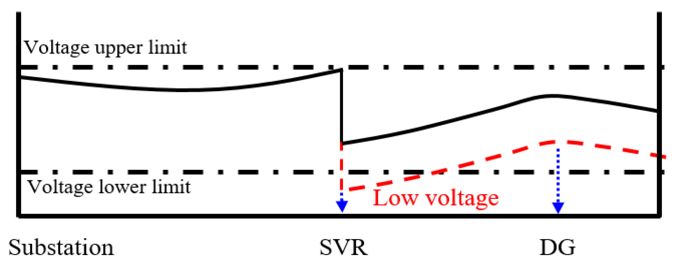
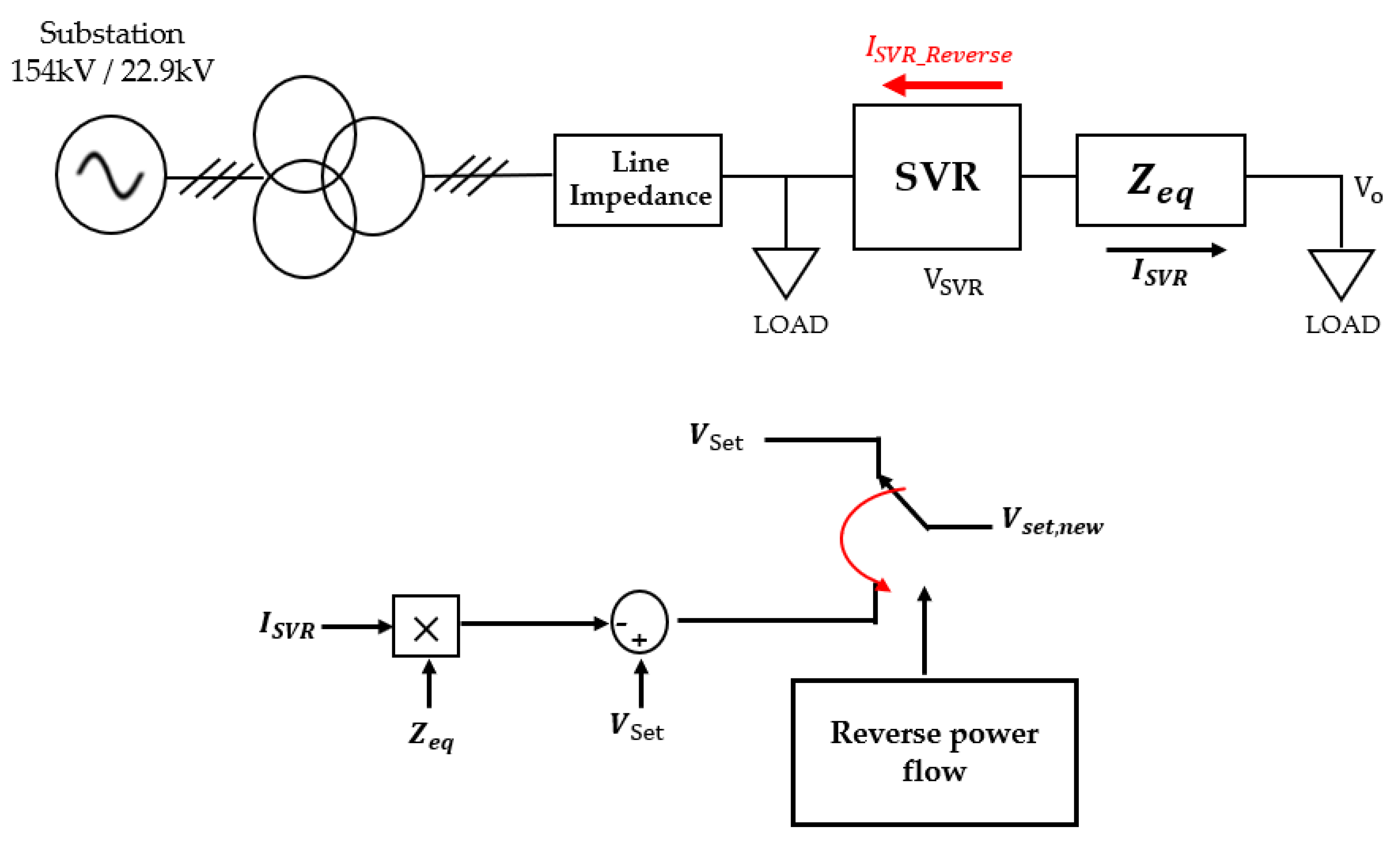
2.3. Reverse Power Flow Control

Now LDC operation of SVR during reverse flow is analyzed. $V_o$ is adjusted to a proper value $V_{Set}$ for forward current $I_{SVR}(>0)$ as Equation (1), which is set to approximately 1.0 p.u. generally. For reverse power flow $I_{SVR}$= $-I_{SVR{,}_{Reserve}}(<0)$. $V_o$ is calculated as Equation (3).

$$V_o=V_{SVR}+Z_{eq}\times I_{SVR,\_Reserve}$$

(3)

Therefore, $V_o$ of Equation (3) becomes to be larger than the $V_{Set}$ and SVR tap operates to reduce $V_o$ to $V_{Set}$ and the $V_{SVR}$ becomes to be lower. From this theory, over-voltage and low-voltage problems may frequently occur in the case of reverse power flow by DG interconnection. To solve these problems, three methods have been proposed: bi-directional mode, neutral mode, and co-generation mode [22,23]. The bi-directional mode controls the $V_o$ on the downstream side, determined by the direction of power flow at SVR. The neutral mode operates the SVR tap position to be 1:1 at the moment of reverse power flow. The co-generation mode adjusts the $V_o$ to a certain value decided by the distribution system operator.

First, for the bi-directional mode, if DG is connected at the secondary side of SVR and injects enough power to reverse power flow at SVR, the source side has changed to the other side and SVR becomes to regulate the voltage on the upstream side. When DG is introduced into after SVR without reverse power at SVR, the calculated $V_o$ is higher than the set value, the SVR changes its tap to lower the voltage, and the voltage at DG increases by the reverse power flow at DG location as shown in Figure 3. In this state, if the DG output continues to increase, SVR will adjust for reducing the secondary voltage by placing its tap in a 1:1 position to become SVR location to be virtual load center by Equation (1). The voltage profile of the distribution line is placed between the upper limit and the lower limit of the permissible range of voltage as the solid line in Figure 3a. However, if numerous DGs are interconnected to reverse power flow at SVR enough to deviate from the 1:1 tap position, the source side has changed to the other side and SVR becomes to regulate the voltage on the upstream side. Then, for the calculated $V_o$ higher than the set value $V_{set}$ SVR changes its tap to a lower voltage and finally reaches the lowest position as the dotted line in Figure 3a because the other side is the utility source and its voltage always keeps almost constant. This causes the voltage downstream of the SVR to be outside the upper limit. On the other hand, if the calculated $V_o$ is lower than $V_{set}$, the SVR changes its tap to a higher voltage. Then, the opposite phenomenon occurs: the SVR reaches the highest position, which causes even lower voltage downstream of the SVR as the dotted line in Figure 3b.

Secondly, the neutral mode fixes the tap position of SVR to be 1:1 in the event of reverse power flow to solve the problems of low-voltage or over-voltage as mentioned above. For example, the dotted line in Figure 4a shows a stable (normal state) case, which is the voltage profile under the neutral mode at the instant of reverse flow compared to the solid line under bi-directional mode. However, depending on load conditions, the voltage profile under neutral mode may result in over-voltage as Figure 4b.

The co-generation mode adjusts the $V_o$ to a corrected value derived from the appropriate value for reverse power. However, it is often fixed and uses the first calculated value because of difficulties in calculating proper voltage settings depending on factors, such as DG’s output, location, and load conditions. For example, the solid line in Figure 5 shows the voltage profile based on a voltage setting value calculated with appropriate values. However, if more DG’s are introduced beyond the proper voltage setting, line voltages become lower as the dotted line in Figure 5.

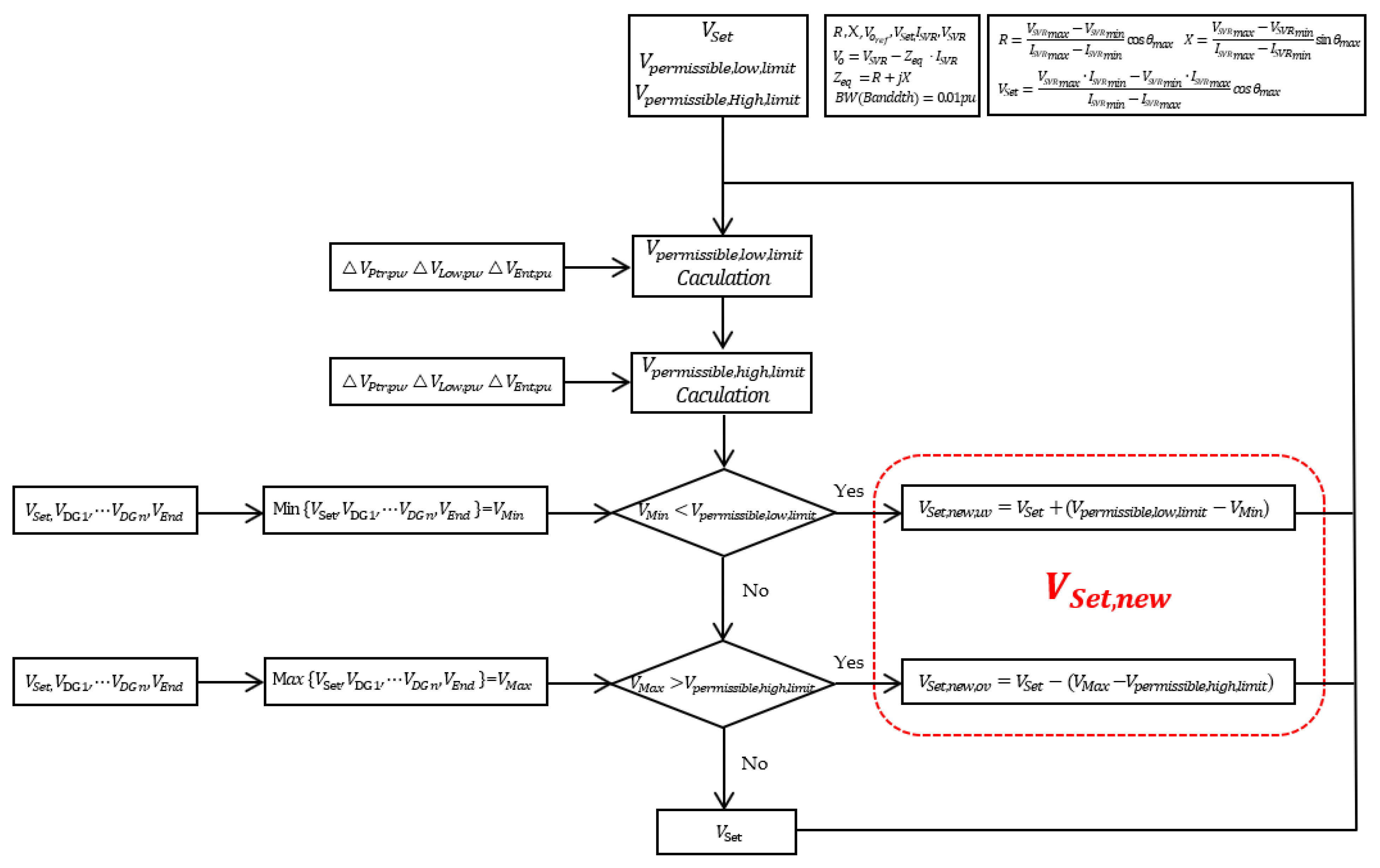
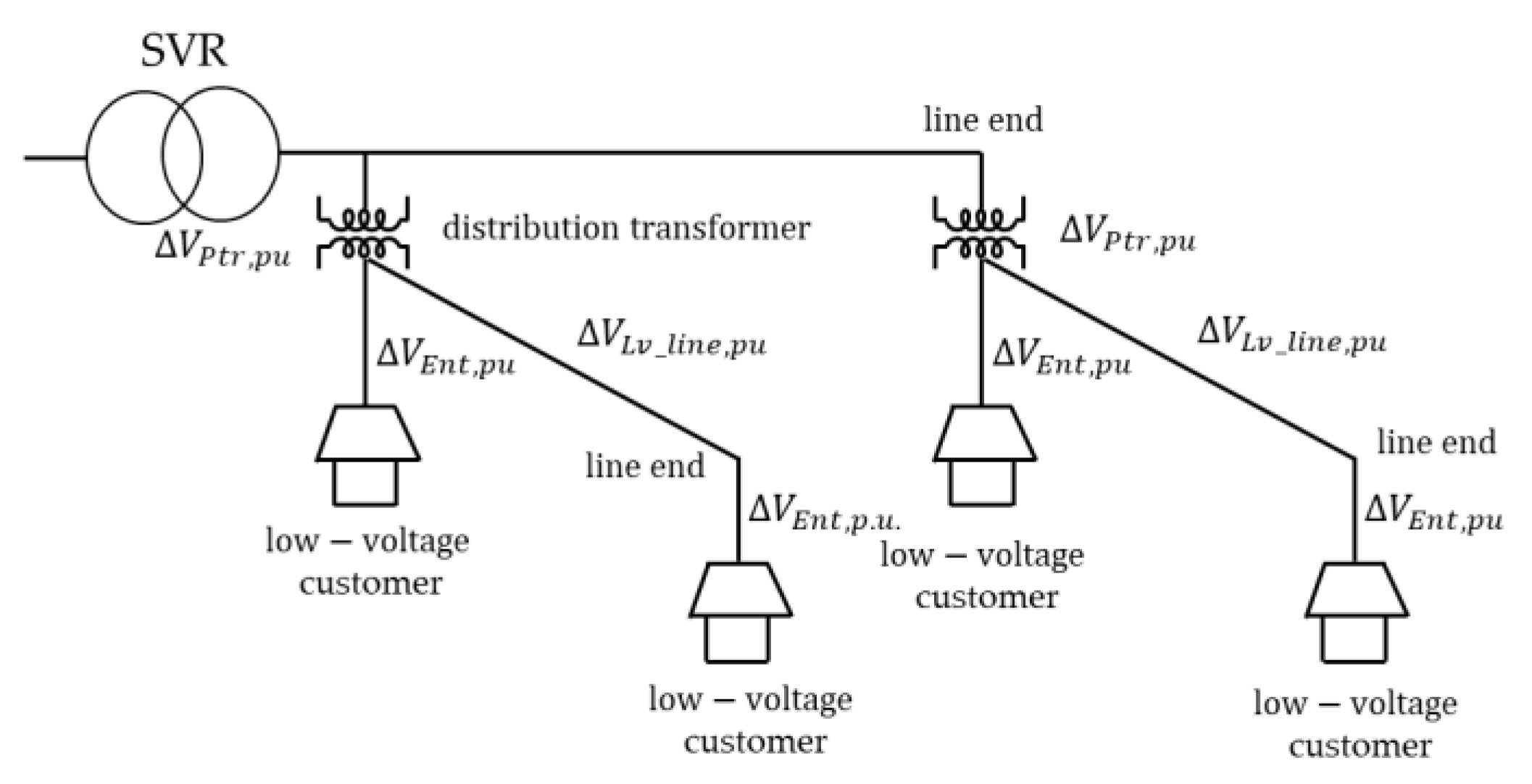
3. SVR Tap-Control Algorithm

As described in Section 2, it is difficult to properly adjust the distribution line’s voltage within permissible ranges owing to DG’s location and its reverse power flow. Especially, we consider the three points most likely to be out of voltage range: the secondary side of SVR, DG’s connection location, and the end of the distribution line. Therefore, this section proposes an advanced SVR tap-control algorithm that determines a proper $V_{set}$ so that the voltage at these three points does not deviate from the permissible range even when DG is interconnected and reverse power flows.

In Figure 6, we consider a distribution line the voltage of which is controlled by SVR and its parameters—$R, X, V_o, V_{set}, BW etc.$ At first, voltage information ($V_{SVR}, V_{DG1},..., V_{DGn}, V_{End}$) for three points is obtained and verified whether these voltages deviate from the upper limit $V_{permissible, high, limit}$ and lower limit $V_{permissible, low, limit}$ decided by the load condition of the distribution line at any time or not. The minimum value is selected as $V_{Min}$ through Min {$V_{SVR}, V_{DG1}, \dots , V_{DGn}, V_{End}$} among the voltage obtained in real-time. If $V_{Min}$ is lower than $V_{permissible, low, limit}$, the $V_{set}$ should be corrected by adding the ($V_{permissible, low, limit}-V_{Min}$) to $V_{Set}$ as shown in Equation (4).

$$V_{Set,new}=V_{Set}+\left(V_{permissible, low, limit}-V_{Min}\right)$$

(4)

In addition, the maximum value $V_{Max}$ is obtained through Max {$V_{SVR}, V_{DG1}, ..., V_{DGn}, V_{End}$}. If $V_{Max}$ is more significant than $V_{permissible, high, limit}$, $V_{set}$ should be corrected by subtracting $\left(V_{Max}-V_{permissible, high, limit}\right)$ from the existing setting $V_{Set}$ as shown in Equation (5).

$$V_{Set,new}=V_{Set}-\left( V_{Max}-V_{permissible, high, limit}\right)$$

(5)

If the voltages at the three points do not exceed the distribution line’s upper and lower voltage limit, the LDC control for SVR is performed with the present value $V_{Set}$. Otherwise, the LDC control for SVR is performed with the new $V_{Set}$ corrected by Equations (4) and (5) so that the voltage on the distribution line is in the permissible voltage range.

This paper also proposes how to obtain $V_{permissible, high, limit}$ and $V_{permissible, low, limit}$ for distribution line as shown in Figure 7. It shows a distribution system composed of a high voltage distribution line, distribution transformer, secondary voltage line, and customer under distribution line after SVR. In Figure 7 a voltage drop of the distribution transformer is denoted by $△V_{Ptr,pu}$, the voltage drop of the low-voltage line by $△V_{LV\_line,pu}$, the voltage drop of customer entrance by $△V_{Ent,pu}$, and the primary-side voltage of the distribution transformer by $V_{High,pu}$. Then the voltage of the low-voltage customer just under the distribution transformer just under the SVR becomes to be $V_{High,pu}-△V_{Ptr,pu}-$ $△V_{Ent,pu}$ and the voltage of the low-voltage customer at the end of the line after the distribution transformer $V_{High,pu}-△V_{Ptr,pu}-V_{LV\_line,pu}-$ $△V_{Ent,pu}$.

If the voltage tolerance of a low-voltage customer is $\pm \alpha$ p.u. and the nominal reference voltage of a low-voltage customer is $V_{Cus,ref,pu}$, the voltage of the low-voltage customer must satisfy Equations (6) and (7) as follow:

$$V_{Cus,ref,pu}-\alpha \le V_{High,pu}-△V_{Ptr,pu}-△V_{Ent,pu}\le V_{Cus,ref,pu}+\alpha$$

(6)

$$V_{Cus,ref,pu}-\alpha \le V_{High,pu}-△V_{Ptr,pu}-△V_{LV\_line,pu}-△V_{Ent,pu}\le V_{Cus,ref,pu}+\alpha$$

(7)

From the above equations, $V_{High,pu}$ must satisfy Equation (8) as follows:

$$\begin{gathered} V_{Cus,ref,pu}-\alpha +△V_{Ptr,pu}+△V_{LV\_line,pu}+△V_{Ent,pu}\le V_{High,pu} \\ \le V_{Cus,ref,pu}+\alpha +△V_{Ptr,pu}+△V_{Ent,pu} \end{gathered}$$

(8)

Based on Equation (8), $V_{permissible,low, limit}$ becomes the left-side and $V_{permissible, high, limit}$ the right-side. They can be obtained depending on load conditions.

Figure 8 explains the voltage profile by the proposed SVR tap-control algorithm when applied to the DG location at peak load, as in Figure 3. In Figure 8, if SVR setting is corrected to be $V_{Set,new,uv}$ as Equation (4) considering dead band, all these will be within permissible voltage ranges illustrated as a red dotted line.

On the other hand, Figure 9 explains the voltage profile by the proposed SVR tap-control algorithm when applied to the DG location at a tolerance load, as in Figure 4. In Figure 9, if SVR setting is corrected to be $V_{Set,new,ov}$ as Equation (5) considering dead band, all these will be within acceptable voltage ranges illustrated as the red dotted line.

4. Simulation and Result

4.1. Simulation and Condition

To verify the tap control algorithm of the proposed SVR, this paper considers a general distribution system with DG composed of 154 kV/22.9 kV transformer and OLTC, four high-voltage distribution lines one of which is relatively long distribution line with SVR. The line lengths are 30 km, 20 km, 10 km, and 4 km, respectively, and each line has four types of load distributions with power factor of 0.8995. This distribution system is modeled as shown in Figure 10 through the PSCAD/EMTDC software tool. The SVR location is where the voltage drop of the line is 10% and the voltage tolerance range of the LV customer is set at 220 ± 6%. A photovoltaic power system with a capacity of up to 13 MVA on Feeder 1 is considered. For impact analysis, DG interconnection point is considered in three cases: at the line end (case I), before the virtual load center (case II), and just after SVR (case III). Detailed data on the distribution system are shown in

Table 1. Specification of the distribution system.

Index	Value	Remark
154 kV Grid Source
Rated Power	50 MVA
Rated Voltage	154 kV
Rated Frequency	60 Hz
Positive Sequence %Z	0.08 + j0.99	100 MVA Based
Zero Sequence %Z	0.34 + j1.69
3-Winding Transformer (154 kV / 22.9 kV / 6.6 kV)
Rated Power	45/60 MVA
Positive Sequence %$X_{1-2}$	j15.97	45 MVA Based
Positive Sequence %$X_{2-3}$	j6.69
Positive Sequence %$X_{3-1}$	j25.38
Connection Type	$Y-Y_g-∆$
Distribution Line (1 km, CNCV-W 325 $m{m}^2$)
Positive Sequence %Z	1.44 + j3.74	100 MVA Based
Zero Sequence %Z	4.46 + j1.56
Distribution Line (1 km, ACSR 160/95 $m{m}^2$)
Positive Sequence %Z	5.23 + j11.62
Zero Sequence %Z	13.65 + j34.2
Local Load	5.95MW + 3.69Mvar	Lagging
Distribution Generation (22.9 kV)
Type of DG	PV
DG Capacity	13 MVA
Transformer Connection	$Y_g-∆$
Positive Sequence %X	j0.05	MVA Based
LDC’s Parameters at Substation OLTC
Equivalent Impedance $Z_{eq}$	1.3262 + j0.8143
Transmission reference voltage $V_{set}$	93.1007 V	120 V Based
LDC’s Parameters at SVR
Equivalent Impedance $Z_{eq}$	19.1657 + j9.369
Transmission reference voltage $V_{set}$	103.8844 V	120 V Based
At Peak Load
Feeder 1 Load Capacity before SVR	3.3975 MVA	p.f. 0.8995
Type 1: Feeder 1 Load Capacity after SVR	2.718 MVA
Type 2: Feeder 1 Load Capacity after SVR	4.077 MVA
Voltage Drop of Distribution Transformer $\mathsf{\Delta }{V}_{Ptr,pu}$	1.913	230 V Based
Voltage Drop of Low-Voltage Line $\mathsf{\Delta }{V}_{L{V}_{line},pu}$	5.739
Voltage Drop of Customer Entrance $\mathsf{\Delta }{V}_{Ent,pu}$	1.913
High-Voltage Line Permissible Range	0.9932 ~ 1.0505 p.u.
At Light load
Feeder 1 Load Capacity before SVR	0.849375 MVA	p.f. 0.8995
Type 3: Feeder 1 Load Capacity after SVR	0.6795 MVA
Type 4: Feeder 1 Load Capacity after SVR	0.3885 MVA
Voltage Drop of Distribution Transformer $\mathsf{\Delta }{V}_{Ptr,pu}$	0.4783	230 V Based
Voltage Drop of Low-Voltage Line $\mathsf{\Delta }{V}_{L{V}_{line},pu}$	1.4348
Voltage Drop of Customer Entrance $\mathsf{\Delta }{V}_{Ent,pu}$	0.4783
High-Voltage Line Permissible Range	0.9216 ~ 1.0219 p.u.

.

Due to the reverse power flow according to introduction of DG’s, a voltage control problem occurs with the $V_{set}$ value in conventional LDC control method. Therefore, this paper proposes a $V_{set}$ value that controls a voltage within the permissible range with Equations (4) and (5). The controller as shown in Figure 11 is modeled through PSCAD/EMTDC. When the controller detects reverse power flow, $V_{set}$ value is adjusted to $V_{set,new}$ value.

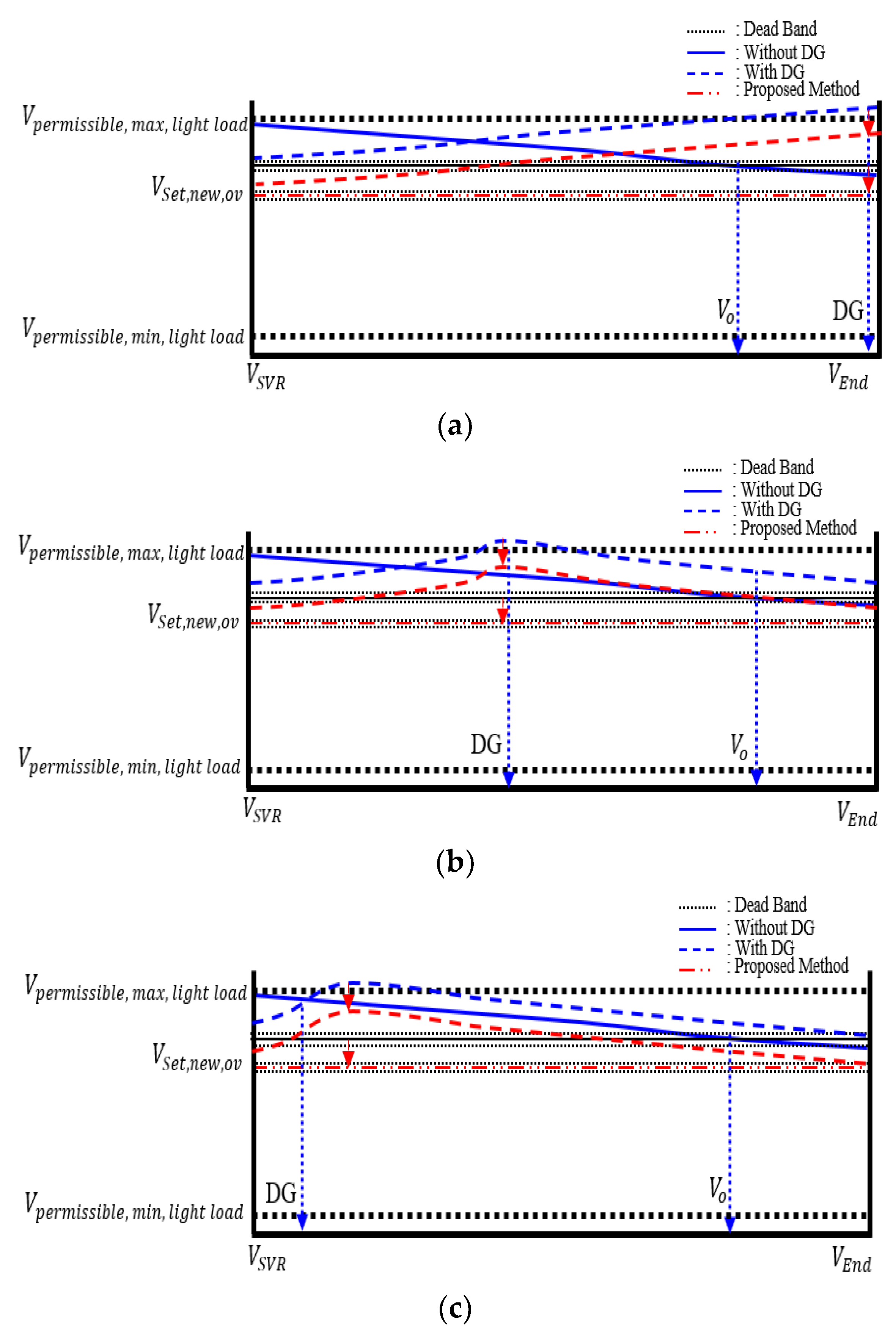
4.2. Simulation and Verification

After SVR, four types of loads are considered to verify the proposed algorithm for various load distributions. Type 1 is set as 2.718MVA, Type 2 as 4.077 MVA, Type 3 as 0.6795 MVA, and Type 4 as 0.3885 MVA. The following results are derived using PSCAD/EMTDC software for each load type and DG introduced location case.

Figure 12 shows the distribution voltage profiles in Type 1 before and after applying the proposed algorithm. As shown in Figure 12a, before applying the algorithm, the voltage profile does not reach the lower voltage limit of 0.9932 p.u. To solve this problem, the proposed algorithm is applied and the $V_{set}$ value at the virtual load center is added as 1.0681 V. Therefore, it is confirmed that the voltage is within the permissible voltage range at the end of the line. As shown in Figure 12b, a voltage does not reach the lower voltage limit of 0.9932 p.u. Therefore, by adding the $V_{set}$ value at the virtual load center as 0.945 V, the voltage is within the permissible range. As shown in Figure 12c, before applying the algorithm, a voltage does not reach the lower voltage limit of 0.9932 p.u. Similarly, the $V_{set}$ value at the virtual load center point is added as 0.9005 V. All cases are confirmed that the voltage is within the permissible range.

Figure 13 shows the distribution voltage profiles in Type 2 before and after applying the proposed algorithm. In this case, the voltage profile is similar compared to Figure 12, however, voltage occurs more quickly. In case I, the line voltage is regulated within the permissible range by adding the $V_{set}$ value as 1.1429 V. In case II, the low-voltage problem is solved by adding a $V_{set}$ value as 1.0106 V. In case III, it is confirmed that the line voltage is within the permissible range by adding the $V_{set}$ value as 1.0327. Therefore, it is verified that the proposed algorithm solves low-voltage problem due to the introduction of loads.

Figure 14 shows the distribution voltage profiles in Type 3 before and after applying the proposed algorithm. As shown in Figure 14a, the voltage problem occurs beyond the voltage upper limit of 1.0219 p.u. in conventional method. To solve this problem, by applying the proposed algorithm, the $V_{set}$ value at the virtual load center is subtracted as 2.8454 V. Therefore, it is confirmed that the voltage is within the permissible voltage range at the end of the line. As shown in Figure 14b, the voltage is beyond the upper limit of 1.0219 p.u. in conventional method. The $V_{set}$ value is subtracted as 3.0547 V to control within the permissible range. Figure 14c shows conventional method, the voltage is beyond the upper limit. Therefore, it is confirmed that the voltage is within the permissible range by subtracting the $V_{set}$ as 3.7598 V in the proposed algorithm.

Figure 15 shows the distribution voltage profiles in Type 4 before and after applying the proposed algorithm. Compared to Figure 14, critical over-voltage occurs due to small-scale loads. In case I, over-voltage problem is adjusted by subtracting $V_{set}$ value as 4.2005 V. In case II, the voltage is regulated within the permissible range by subtracting $V_{set}$ value as 3.3742 V. In case III, it is confirmed that the voltage is within the permissible range by subtracting $V_{set}$ value as 2.7903 V. It is verified that when large-scale DG is introduced, the problem of critical over-voltage is regulated through the proposed algorithm.

The proposed algorithm is to adjust the $V_{set}$ value at the virtual load center point to solve the over or low-voltage problem when large-scale DG’s are introduced. By the $V_{set,new}$ in Figure 6, the voltage profiles as shown in Figure 12 to Figure 15 are within permissible voltage range. Therefore, it is known that our algorithm is effective to properly regulate the distribution voltage.

5. Conclusions

As energy transition takes place around the world, the interconnection of large-scale DG into distribution systems is increasing and bi-directional power flow occurs more. This causes over or low-voltage problems. Generally, there are three types of conventional operation methods for SVR installed on long distribution lines: LDC, constant voltage control, and reverse power flow mode. In those methods, it is difficult to control the line voltage within permissible ranges when reverse power flows by DG introduction. This problem will continue to increase according to the DG capacity and load connected to the distribution line. Therefore, a new control method of SVR is required.

Therefore, this paper proposed a novel tap-change algorithm of SVR considering large-scale DG introduced into distribution systems with long distribution lines. The proposed algorithm can solve over or low-voltage problems.

To verify this algorithm, typical distribution systems were modeled through PSCAD/EMTDC software tool, and the proposed tap change algorithm was applied. Then, it was confirmed that the voltage profile of the 22.9 kV distribution line at peak load and light load is within permissible voltage ranges when large-scale DG is introduced. Consequently, our proposed method improved the conventional LDC voltage control method in distribution systems with long distribution line and large-scale DG.

As a result, the tap change algorithm of SVR proposed in this paper is expected to be applied and solve the voltage problem in distribution systems with large-scale grid interconnection of DG. However, if faults occur and circuit breaker opens, all DG’s are disconnected. The breaker recloses after fault elimination and then voltage profiles become to be beyond permissible voltage range. The LDC controller at substation and the SVR operate simultaneously, and their operation is hunting so that voltage regulation cannot be performed properly. This is to be solved in a future study.

References

1. IPCC. Summary for Policymakers. 2018. Available online: https://www.ipcc.ch/sr15/chapter/spm/ (accessed on 6 October 2018).
2. Kraiczy, M.; AL Fakhri, L.; Braun, M. Local Voltage Support by Distributed Generation; IEA-PVPS T14-08; International Energy Agency: Paris, France, 2017. [Google Scholar]
3. Mahmud, N.; Zahedi, A. Review of Control Strategies for Voltage Regulation of the Smart Distribution Network with High Penetration of Renewable Distributed Generation. Renew. Sustain. Energy Rev. 2016, 64, 582–595. [Google Scholar] [CrossRef]
4. Hu, J.; Li, Z.; Zhu, J.; Guerrero, J. Voltage Stabilization. IEEE Ind. Electron. Mag. 2019, 13, 17–30. [Google Scholar] [CrossRef]
5. IEEE-PES Task Force on Voltage Control for Smart Grids. Review of Challenges and Research Opportunities for Voltage Control in Smart Grids. IEEE Trans. Power Syst. 2019, 34, 2790–2801. [Google Scholar] [CrossRef] [Green Version]
6. Liu, Y.; Guo, L.; Lu, C.; Chai, Y.; Gao, S.; Xu, B. A Fully Distributed Voltage Optimization Method for Distribution Networks Considering Integer Constraints of Step Voltage Regulators. IEEE Access 2019, 7, 60055–60066. [Google Scholar] [CrossRef]
7. Sgouras, K.I.; Bouhouras, A.S.; Gkaidatzis, P.A.; Doukas, D.I.; Labridis, D.I. Impact of Reverse Power Flow on the Optimal Distributed Generation Placement Problem. IET Gener. Transm. Distrib. 2017, 11, 4626–4632. [Google Scholar] [CrossRef]
8. NamKoong, W.; Jung, W.-W.; Shin, C.-H.; Hwang, P.-I.; Jang, G. Voltage Control of Distribution Networks to Increase their Hosting Capacity in South Korea. J. Electr. Eng. Technol. 2021, 16, 1305–1312. [Google Scholar] [CrossRef]
9. Nagarajan, L.; Senthilkumar, M. Power Quality Improvement in Distribution System Based on Dynamic Voltage Restorer Using Rational Energy Transformative Optimization Algorithm. J. Electr. Eng. Technol. 2022, 17, 121–137. [Google Scholar] [CrossRef]
10. Jahn, R.; Holt, M.; Rehtanz, C. Mitigation of Voltage Unbalances Using a Line Voltage Regulator. In Proceedings of the 2021 IEEE Madrid PowerTech, Madrid, Spain, 28 June 2021; pp. 1–6. [Google Scholar]
11. Yan, R.; Li, Y.; Saha, T.K.; Wang, L.; Hossain, M.I. Modeling and Analysis of Open-Delta Step Voltage Regulators for Unbalanced Distribution Network with Photovoltaic Power Generation. IEEE Trans. Smart Grid 2018, 9, 2224–2234. [Google Scholar] [CrossRef] [Green Version]
12. Nakadomari, A.; Shigenobu, R.; Senjyu, T. Optimal Control and Placement of Step Voltage Regulator for Voltage Unbalance Improvement and Loss Minimization in Distribution System. In Proceedings of the 2020 IEEE Region 10 Conference, Osaka, Japan, 16–19 November 2020; pp. 1013–1018. [Google Scholar]
13. Liu, E.; Bebic, J. Distribution System Voltage Performance Analysis for High-Penetration Photovoltaics; NREL/SR-581-42298; National Renewable Energy Lab: Golden, CO, USA, 2008. [Google Scholar]
14. Bai, F.; Yan, R.; Saha, T.K.; Eghbal, D. A New Remote Tap Position Estimation Approach for Open-Delta Step-Voltage Regulator in a Photovoltaic Integrated Distribution Network. IEEE Trans. Power Syst. 2018, 33, 4433–4443. [Google Scholar] [CrossRef] [Green Version]
15. Ranamuka, D.; Agalgaonkar, A.P.; Muttaqi, K.M. Online Voltage Control in Distribution Systems with Multiple Voltage Regulating Devices. IEEE Trans. Sustain. Energy 2014, 5, 617–628. [Google Scholar] [CrossRef]
16. Chamana, M.; Chowdhury, B.H.; Jahanbakhsh, F. Distributed Control of Voltage Regulating Devices in the Presence of High PV Penetration to Mitigate Ramp-Rate Issues. IEEE Trans. Smart Grid 2018, 9, 1086–1095. [Google Scholar] [CrossRef]
17. Chamana, M.; Chowdhury, B.H. Optimal Voltage Regulation of Distribution Networks with Cascaded Voltage Regulators in the Presence of High PV Penetration. IEEE Trans. Sustain. Energy 2018, 9, 1427–1436. [Google Scholar] [CrossRef]
18. Tonkoski, R.; Turcotte, D.; El-Fouly, T.H. Impact of high PV penetration on voltage profiles in residential neighborhoods. IEEE Trans. Sustain. Energy 2012, 3, 518–527. [Google Scholar] [CrossRef]
19. Baran, M.E.; Wu, F.F. Network reconfiguration in distribution systems for loss reduction and load balancing. IEEE Power Eng. Rev. 1989, 4, 101–102. [Google Scholar] [CrossRef]
20. Abrar Ahmed, C.; Vinod, K. DC-Microgrid Voltage Regulation using Dual Active Bridge based SVR. In Proceedings of the 2021 7th International Conference on Electrical Energy Systems (ICEES), Chennai, India, 11–13 February 2021; pp. 490–495. [Google Scholar]
21. Short, T.A. Electric Power Distribution Handbook; CRC Press: New York, NY, USA, 2014; pp. 734–739. [Google Scholar]
22. Wareham, D. Step Voltage Regulators, Cooper Power Systems by EATON. 2013. Available online: http://www.cscos.com/wp-content/uploads/NY1839-Eaton-Regulators-D.Wareham.pdf (accessed on 15 October 2022).
23. Kajita, H.; Kanbe, A.; Fugawa, K.; Kadokura, S. Development of SVR Control System for Dispersed Power Supply; 2005 Aichi Electric Technical Report No.26; Aichi Electrical: Nagoya, Japan, 2005; pp. 10–16. (In Japanese) [Google Scholar]
Figure 1. The concept of LDC control method.
Energies 15 09579 g001
Figure 2. Operation Structure of LDC.
Energies 15 09579 g002
Figure 3. Voltage Profiles under Bi-directional Mode: (a) Over-voltage Case; (b) Low-voltage Case.
Energies 15 09579 g003
Figure 4. Voltage Profiles under Neutral Mode.
Energies 15 09579 g004
Figure 5. Voltage Profiles under co-generation mode.
Energies 15 09579 g005
Figure 6. Proposed SVR tap-control Algorithm when reverse power flows.
Energies 15 09579 g006
Figure 7. Distribution Line Downstream after SVR.
Energies 15 09579 g007
Figure 8. Voltage Profile by proposed SVR tap-control algorithm at peak load: (a) Case I; (b) Case II; (c) Case III.
Energies 15 09579 g008aEnergies 15 09579 g008b
Figure 9. Voltage Profile by proposed SVR tap-control algorithm at light load: (a) Case I; (b) Case II; (c) Case III.
Energies 15 09579 g009
Figure 10. Modeling of the distribution system.
Energies 15 09579 g010
Figure 11. V s e t , n e w Controller for the proposed algorithm.
Energies 15 09579 g011
Figure 12. Distribution line voltage profiles by conventional and proposed voltage control in Type 1: (a) Case I; (b) Case II; (c) Case III.
Energies 15 09579 g012
Figure 13. Distribution line voltage profiles by conventional and proposed voltage control in Type 2: (a) Case I; (b) Case II; (c) Case III.
Energies 15 09579 g013
Figure 14. Distribution line voltage profiles by conventional and proposed voltage control in Type 3: (a) Case I; (b) Case II; (c) Case III.
Energies 15 09579 g014
Figure 15. Distribution line voltage profiles by conventional and proposed voltage control Type 4: (a) Case I; (b) Case II; (c) Case III.
Energies 15 09579 g015