Abstract
This work aims to assess the impacts of climate change on photovoltaic (PV) electricity in two Italian cities, with different latitudes and Köppen–Geiger climate classifications. This was undertaken using the recent EURO-CORDEX set of high-resolution climate projections and PV power generation models, implemented on TRNSYS software. Data for two variables (surface air temperature and solar radiation) were analysed over a long period from 1971 to 2100. For future periods, two of the Representative Concentration Pathway scenarios (RCP4.5 and RCP8.5) used in the Intergovernmental Panel on Climate Change Fifth Assessment Report were considered. In both RCP scenarios and both locations, it is estimated that the yearly PV energy produced in the future period will not undergo significant variations on average given that the rate of decrease is foreseen almost constant; instead, a slight reduction in the PV energy was detected in the past period. It can be concluded that the PV market in Italy will grow in the next years considering that the reduction in the foreseen PV purchase costs will be also supported by the slight positive effect of climate change on PV manufacturability.
1. Introduction
Renewable energy bridges the gap between climate and energy science. Renewable energy plays a key role in mitigation strategies aimed at reducing the effects of climate change on societies and the environment [1]. Nevertheless, most renewable resources are in turn dependent on weather and climate, a dependence that could affect the feasibility of future low-carbon energy supply systems [2]. A sustainable future requires understanding and quantifying the effect of climate change on energy production [3]. Among the various renewable energy sources, one of the most important appears without a doubt to be photovoltaics (PVs). It depends on solar irradiation, referred to as shortwave radiation (i.e., 0.3–1.1 μm wavelength range), climate patterns, and other atmospheric variables that affect panel efficiency, such as air temperature. One of the main parameters is the operating temperature of PV modules [4]. Study [5] investigated through techno-economic analysis the temperature management of PV modules. The phenomenon of dirt resulting from the deposition of dust particles on solar energy equipment and systems is becoming increasingly significant; a layer of dust covering the surface of PV modules reduces PV electricity production by shielding solar radiation [6].
A recent report by the Intergovernmental Panel on Climate Change (IPCC) [7] states that summer heatwaves or intense precipitation are now much more frequent than they were in the middle of the 20th Century, and it is possible to say that these are the direct consequence of the rapid global warming of the last 150 years [8]. This organization aims to assess, based on scientific, technical and socio-economic data and evidence, the risk of human-induced climate change and its possible consequences and also can suggest possible solutions for the reduction of these changes. Moreover, based on data provided by the IPCC, it is demonstrated that the amount of solar energy that is absorbed by our planet is always increasing, and therefore the Earth, not being in thermal equilibrium, is destined to become warmer and warmer in the coming years and decades. The relationship between climate change and extreme weather events is becoming more and more defined, as well as the relationship between greenhouse gas emissions and climate change. During the last 20 years, the conclusions reached by the IPCC are more and more certain, and today, the main cause of climate change is 95% caused by greenhouse gas emissions. If the man is a cause, it is the man who must act to avoid even more catastrophic damage.
1.1. Representative Concentration Pathway Scenarios
Continued emissions of greenhouse gases will cause further warming and changes in all components of the climate system. Limiting climate change will require substantial reductions in greenhouse gas emissions. Warming will continue to exhibit interannual and decadal variability and will not be regionally uniform. Total CO2 emissions will largely determine average surface global warming in the late 21st Century and beyond. Most climate change trends will persist for many centuries, even if CO2 emissions can be stopped. In essence, this latest IPCC conclusion implies that the fight against climate change created by past, present, and future CO2 emissions is inevitably long-lasting and multi-century and that many changes will be irreversible. In the Fifth IPCC Assessment Report (AR5) [9], four new Representative Concentration Pathways (RCP) scenarios are calculated that also consider the effects of mitigation policies. These scenarios are identified by the value of the approximate total radiative forcing in 2100, compared to 1750: 2.6 W/m2 for RCP 2.6; 4.5 W/m2 for RCP4.5; 6.0 W/m2 for RCP 6.0; and 8.5 W/m2 for RCP8.5. For the results under the Coupled Model Intercomparison Project Phase 5 (CMIP5), these values should only be understood as indicative, since the resulting climate forcing from all drivers varies for different models due to their specific characteristics and treatment of short-lived climate forcings. Ultimately, the scenarios can be summarized as follows:
- RCP 2.6 is a mitigation scenario (high effort to curb emissions; renewable energy generation; emission capture; bicycles, electric cars and public transport; average temperature increase of 1 °C; average rise of sea level of 0.4 m; small increase in extreme weather; low level of adaptation and low costs required);
- RCP4.5 is a stabilization scenario (medium effort to curb emissions; renewable energy generation; bicycles, petrol and electric cars and trucks for the transport sector; average temperature increase of 1.8 °C; average rise of sea level of 0.47 m; moderate increase in extreme weather; medium level of adaptation and medium costs required);
- RCP 6.0 is a stabilization scenario (medium effort to curb emissions, coal-fired and renewable energy generation; bicycles, petrol and electric cars and trucks for the transport sector, average temperature increase of 2.2 °C; average rise of sea level of 0.48 m; moderate increase in extreme weather; medium level of adaptation and medium costs required);
- RCP8.5 is a high emissions scenario (low effort to curb emissions; coal-fired energy generation; petrol cars and trucks for the transport sector; average temperature increase of 3.7 °C; average rise of sea level of 0.63 m; large increase in extreme weather; high level of adaptation and high costs required).
- These RCP scenarios were used in different energy fields. For example, Tettey et al. analysed the final and primary energy savings and overheating risk of the deep energy renovation of a Swedish multi-storey residential building in the 1970s under climate change [10]. Instead, the objective of other research was to propose a method to evaluate the impact of climate change inside religious historical spaces and its impact on thermal comfort, the preservation of artworks, and energy consumption [11].
1.2. How the Performance of Photovoltaic Systems Is Affected by Climate Change
When renewable energy sources and climate change are considered in the same context, the analysis focuses on the impacts that renewable energy could have on climate change mitigation through the reduction of greenhouse gas emissions. In these studies, the research focus is different: they attempt to identify how future climate change might impact renewable energy production. Solar cells need sunlight to generate electricity, but with light also comes heat. On a warming planet, scientists warn that temperatures may become too high for PV panels to operate efficiently. Malvoni et al. [12] investigated the performance of a 960 kWp PV system located in southern Italy. Monitoring data over a period of 43 months are used to evaluate the monthly average of energy yields, losses, and efficiency. A warming scenario projected by the IPCC estimates that global temperature will increase by 1.8 °C by 2100, leading to median reductions in annual energy production of 15 kWh/kWp, with reductions of up to 50 kWh/kWp in some areas where temperature increases will be greatest [13]. There are several physical reasons why the efficiency of a solar cell is a function of temperature. Simplifying, it can be said that as temperature increases, there is a reduction in open circuit voltage, thus hindering the process of electron liberation inside the PV cell and consequently decreasing its efficiency of conversion into electricity. As suggested by the research, thanks to the possible discoveries at the level of materials, in the future, PV panels can be much more efficient than the current ones. Ultimately, then, it can be said that any efficiency reductions attributable to rising temperatures will be largely “overshadowed” by technological improvements and the skyrocketing growth of new PV installations. Estimated changes in energy production, based on relatively coarse resolution global simulations [14,15], indicate small but generally positive impacts of climate change on PV system performance over Europe under both the SRB A1B and RCP8.5 scenarios [16]. Other local studies found a slight increase in solar radiation in the UK and Greece [17] and negligible signals in northwest Germany. However, the impact of climate change on PV generation, including the impact on temporal stability, is still very poor.
This paper aims to provide an overview of the direct effects of climate change on PV generation over two Italian locations considering a future period with a high penetration of PV systems. For this, the most up-to-date set of high-resolution Regional Climate Model (RCM) projections was used, namely, the EURO-CORDEX. Specifically, an RCM was used to rescale a global climate model (GCM) under two climate scenarios (RCP4.5 and RCP8.5). The time series of two variables, surface downwelling shortwave radiation (RSDS) and near-surface air temperature (TAS), extrapolated from the Web Portal, from which the climatic data of the EURO-CORDEX project can be freely downloaded, were used to estimate the time series of the electric power produced by PVs. Through the climatic variables, it was already possible to have an idea of how climate change will affect the performance of PV systems in the two Italian locations considered.
2. Materials and Methods
This section presents the methodology followed in the present study. Figure 1 illustrates each step of the analysis.
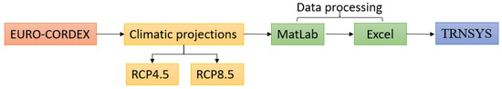
Figure 1.
Flow chart containing all the steps followed for the analysis.
2.1. Climate Models
A climate model is a set of mathematical equations that represent the physical laws that describe the evolution of the climate system. All climate models consider both the radiation coming from the Sun in the form of electromagnetic radiation, mainly in the visible and near-infrared, and the radiation leaving our planet in the form of infrared radiation at longer wavelengths. The equilibrium is governed by the laws of thermodynamics and gives rise to temperature variations. The most advanced climate models try to take into account all the factors involved in the regulation of the climate system. Such models, once built, run on supercomputers and are validated based on past climate data by running the model back in time and verifying the goodness or otherwise of the climate simulated with that present in the historical series.
The models differ in the complexity of their structures:
- The simple model based on radiant heat transfer considers the Earth as a single point with uniform energy output. This model can be expanded both vertically (radiative-convective models) and horizontally.
- Models that couple atmosphere–ocean–cryosphere circulation fully solve the equations for energy and mass transfer and heat transfer.
- Box models deal with flow across and within ocean basins.
- Other modelling uses interconnections such as land use to assess climate–ecosystem interactions.
On the strict implementation side, i.e., in the model application, scientists divide planet Earth into a three-dimensional grid and evaluate the results of the final computation on it: atmospheric models calculate winds, heat transfer, solar radiation, relative humidity, and surface hydrology within each grid, taking into account interactions with neighbouring points.
GCM, RCM and Dynamic Downscaling Models
The tool used for the simulation of possible future climate scenarios is given by the so-called Global Climate Model (GCM). A large set of climate projections was used in the Fourth Assessment Report (AR4) prepared by 18 modelling groups worldwide, which conducted several coordinated climate experiments in which several GCMs were run for a common set of experiments and various scenarios of greenhouse gases [18]. Research communities can use these data sets to assess the impact of changing climate on various systems of interest by accessing the IPCC Data Distribution Centre (www.ipcc-data.org, (accessed on 18 October 2022)). In the latest generations of GCMs, the atmospheric component is combined with oceanic models and models of the glacial shield, vegetation, and land surface. In GCMs, according to the state of the art, the Earth’s surface is divided into a grid of 100–200 km, sometimes even narrower. In addition, the atmosphere and the ocean are divided into 20–40 vertical layers. In the resulting three-dimensional lattice, processes relevant to the atmosphere, such as wind circulation, cloud and precipitation formation, energy transfers, and all exchange processes taking place between the land surface, ocean, and vegetation, are calculated using mathematical equations at the rate of several minutes. The results of these calculations should be a realistic approximation of the processes affecting the Earth system. As noted, GCMs can provide an overview of the climate and climate change of the entire planet, but because of their relatively approximate horizontal resolution, they are of little use when focused on small areas.
For this reason, RCMs have also been developed [19]. RCMs work by increasing the resolution of the GCM over a small, limited area of interest. An RCM might cover an area the size of Western Europe or southern Africa, typically 5000 km × 5000 km. The full GCM determines the large-scale effects of changing greenhouse gas concentrations and volcanic eruptions on the global climate. The climate calculated by the GCM is used as input to the RCM edges for factors such as temperature and wind. RCMs can then resolve local impacts given small-scale information on orography (land elevation) and land use, providing weather and climate information with resolutions down to 50 or 25 km. In regions where the Earth’s surface is flat for thousands of kilometres and there is no nearby ocean, the approximate resolution of a GCM may be sufficient to accurately simulate climate change. However, most land areas have mountains, coastlines, and changes in vegetation characteristics on much smaller scales, and RCMs can represent the effects of these on climate much better than GCMs. The forcing of an RCM by a GCM is known as Dynamic Downscaling [20]. Therefore, dynamic downscaling uses an RCM with a higher spatial resolution over a limited area and is fed large-scale weather conditions from the GCM. As there are many regional climate simulations available, research and several modelling activities have been created, including a common interface for applicants.
The Coordinated Regional Climate Downscaling Experiment (CORDEX) aims to compare, improve, and standardize regional climate modelling in individual modelling centres around the world, thus harmonizing the new generation of regional climate projections by applying the latest versions of RCM ensembles, driven by the latest GCM projections with unprecedented high resolutions (e.g., simulations with 0.11° resolution are available for Europe, which means about a 12 × 12 km grid size) [21,22]. Therefore, the EURO-CORDEX framework was considered in this work. This project provides regional climate projections for the European CORDEX domain, thus complementing the previous PRUDENCE (terminated in 2004) and ENSEMBLES (terminated in 2009) experiments.
2.2. EURO-CORDEX Project
The World Climate Research Program (WCRP) established the Task Force on Regional Climate Downscaling (TFRCD) in 2009, which created the Coordinated Regional Climate Downscaling Experiment (CORDEX) initiative to generate regional climate change projections for all terrestrial regions of the globe within the timeline of the IPCC AR5. The primary goals of the CORDEX initiative are to provide a coordinated model assessment framework, climate projection framework, and interface for applicants for climate simulations in studies of climate change impacts, adaptation, and mitigation.
As part of the overall CORDEX framework, the EURO-CORDEX initiative provides regional climate projections for Europe at a resolution of 50 km (EUR-44) and 12.5 km (EUR-11), thereby integrating coarser-resolution datasets from previous activities, such as PRUDENCE and ENSEMBLES (the ENSEMBLES project covered RCM simulations for Europe at a maximum resolution of 25 km and, in PRUDENCE, all simulations were run on a 50 km grid). Thus, EURO-CORDEX is the European branch of the CORDEX initiative that enables the production of ensemble climate simulations based on multiple dynamical and empirical-statistical downscaling models forced by multiple global climate models from Phase 5 of the Coupled Model Intercomparison Project (CMIP5).
The EURO-CORDEX simulations consider global climate simulations from the long-term CMIP5 experiments through the year 2100. They are based on RCPs defined in the IPCC AR5. In contrast to the SRES scenarios, the RCP scenarios do not specify socioeconomic scenarios but assume paths toward different target radiative forcings at the end of the 21st Century. For example, the RCP8.5 scenario assumes an increase in radiative forcing of 8.5 W/m2 by the end of the 21st Century relative to pre-industrial conditions.
2.2.1. EURO-CORDEX Publications
The EURO-CORDEX Project has been used to carry out many studies that aim at improving climate projections, and some of these studies have been taken into account for the realization of this work. For example, a study was carried out that focuses on the initial assessment of climate change impacts on renewable energy sources in Croatia, specifically PV, wind, and hydropower. The climate data used for this assessment were taken from the global climate model ECHAM5-MPIOM and dynamically downscaled from the RCM at the Croatian Meteorological and Hydrological Service (DHMZ). The results based on the IPCC A2 scenario for the two future climate periods 2011–2040 and 2041–2070 are analysed [9]. Another study considered presents two models that assess the impacts of climate change on solar and wind power generation, using them to evaluate climate projections based on the A1B scenario for the north-western metropolitan region of Germany [10]. In a further study, a consistent set of climate projections was developed and evaluated for high space and time resolutions that address the problem of using climate projections that have remained limited to date for several reasons, including a lack of consistency among climate projections, climate model biases, a lack of user guidance, and dataset size. Here, the dataset includes eleven EURO-CORDEX simulations at a 12 km resolution of hourly and daily temperature, precipitation, wind speed, and surface solar radiation [11].
2.2.2. Earth System Grid Federation (ESGF)
An initial focus of the CORDEX initiative was the creation of a central CORDEX archive, supplemented by regional data portals. However, it soon became clear that a geographically distributed archive system would offer much greater flexibility for the delivery of numerous CORDEX RCM simulations produced by many modelling groups around the world, similar to CMIP5. For this reason, the Earth System Grid Federation (ESGF) was born [23]. ESGF is an up-to-date scientific infrastructure for climate data distribution and has now become WCRP’s primary tool for providing global and regional climate simulations along with observations and analysis over the next decade. Through ESGF, users access, analyse and view data using a globally federated collection of networks, computers, and software. Once the desired project dataset is selected and downloaded, a file in the NetCDF (Network Common Data Form) format can be obtained. This is a file format used for storing multidimensional (variable) scientific data, which can be viewed across a dimension (such as time) by creating a layer or table view from the NetCDF file. Connected to the Earth System Grid Federation infrastructure is the Climate4impact portal. The portal aims to support climate change impact modellers, impact and adaptation consultants, and anyone else who wishes to use climate change data. The portal provides Web interfaces for searching, viewing, analysing, processing, and downloading datasets.
2.3. Model CCLM 4-8-17EC Earth
2.3.1. Climate Variables
In this study, a limited set of climate variables, TAS and RSDS, selected taking into account studies carried out by different energy professionals, was considered for their use after processing these variables. TAS is used in several applications: to model energy demand for heating or cooling, to estimate evapotranspiration in hydrological models that estimate hydropower inflow, and to modulate solar PV energy production since solar panels have temperature-sensitive efficiencies. Surface solar radiation, also called downwelling solar radiation at the surface, is needed to estimate PV energy production.
2.3.2. Climate Projections
Two RCP scenarios were considered: RCP4.5 (median) and RCP8.5 (pessimistic). In addition to analysing future data, historical data were also considered so that comparisons could be drawn. Once the known fields were checked on the ESGF portal, 229 results were obtained, in a total of 38 GCM-RCM models. The first selection of models was made based on their completeness, as not all of them incorporate both models and both RCP scenarios; 38 models were reduced to 18 models. A second skimming was performed considering the data visualization on the Climate4impact portal. For 3 RCM models (ALADIN 53, ALADIN 63, and HIRHAM 5), the visualization was found to be poor and, consequently, it would not have been possible to check the data. Ultimately, among the 15 remaining models, the model found to be most suitable is CCLM 4-8-17—EC EARTH since it provides intermediate values of climate variables (TAS and RSDS) among all models. This was verified in some localities for some future periods.
2.3.3. CCLM 4-8-17—EC EARTH Model
The CCLM model (short for COSMO-CLM) is the climate version of the COSMO LM model, which is the operational non-hydrostatic weather prediction model initially developed by the German weather service DWD and then by the European COSMO consortium. COSMO-CLM is used with a spatial resolution between 1 and 50 km; these values are generally close to those required by impact modellers; in fact, they allow the description of the terrain orography more correctly than global models. The mathematical formulation of COSMO-CLM is based on the fluid dynamic equations for a compressible flow. The atmosphere is treated as a multi-component fluid (composed of dry air, water vapour, liquid water, and solid) for which the perfect gas equation applies and is subject to gravity and Coriolis forces. For the RCM model CCLM4-8-17 with a driving model EC-Earth, the historical data are available from 1950 to 2005. Instead, data for future periods are available from 2006 to 2100. In this study, the past historical period is represented by data from 1971 to 2005, while the future period is by data from 2021 to 2100. Instead, data between 2006 and 2020 are past data that are simulated and cannot be considered historical.
3. Data Processing
3.1. Climate Data
Once the regional model (COSMO-CLM) to be grafted on the two scenarios, RCP4.5 and RCP8.5, was chosen from the global climate model EC-EARTH, the 48 NetCDF files containing the monthly average hourly data of RSDS, expressed in W/m2, and TAS, expressed in K, were downloaded for the period from January 1971 to December 2100. Each NetCDF file contains data for 10 years. MatLab software was chosen to open and convert these files. Each file downloaded from the web portal contains within it many variables, such as, in addition to TAS or RSDS, time, latitude and longitude. After the conversion, a three-dimensional matrix is created for each NetCDF file. In the case, for example, of the file inherent in the TAS variable with RCP4.5, referring to the period from January 2011 to December 2020, a 424 × 412 × 120 matrix was obtained. It is, therefore, 120 matrices of 424 × 412, where 120 indicates the 12 months of the 10 years. The next step was to print all the data from the 424 × 412 × 120 matrix onto an Excel spreadsheet by means of a script on MatLab. The Excel file contained 120 sheets, each with a 424 × 412 matrix. These same steps were performed for each NetCDF file. Ultimately, all temperature and solar radiation values for 130 years were obtained for both RCP scenarios considered. The visualization of the data on the Climate4impact portal Data is a pixelated map with 174, 688 pixels, each of 12.5 km resolution, covering the whole of Europe. Each pixel represents a value of TAS, RSDS, latitude, and longitude. Going from the bottom to the top of the maps, the rows of the matrices are scrolled and going from left to right, the columns are scrolled.
3.2. Case Study
In this work, two Italian localities, Rome in the Csa (Mediterranean hot summer) Köppen climate classification and Milan in the Cfa (Humid subtropical) Köppen climate classification, were chosen [24]. In recent years, PV research has focused on both small-medium and large system sizes for different sectors in Italy [25,26,27,28]. Data on solar radiation and air temperature in past and future periods were used to calculate the hourly electrical power produced by a PV module to identify the effect of climate change on the performance of the PV module. To calculate the hourly power produced by a PV module, given the values of temperature and solar radiation, the TRNSYS software was used [29]. As shown in the TRNSYS scheme of Figure 2, the following types were used:
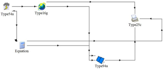
Figure 2.
TRNSYS scheme.
- Type 54a generates hourly meteorological data given the monthly average values of solar radiation, dry bulb temperature, and humidity ratio.
- Type 16g interpolates radiation data, calculates various quantities related to the Sun’s position, and estimates radiation on a range of surfaces of fixed or variable orientation.
- Type 94a models single or polycrystalline silicon PV panels to estimate their electrical performance.
- Type 25c is a subroutine for printing to output files from other types.
The electrical characteristics of the polycrystalline PV module, Jakson 250, are shown in Table 1. All these electrical characteristics are provided by the manufacturer [30] and are required in the TRNSYS from type 94. For both localities, the optimal PV inclination angle that maximizes the electrical energy produced was considered. The optimal angle obtained by means of preliminary simulations in Rome is 33°, while in Milan, it is 36°. A parametric hourly simulation was performed for each locality and each RCP scenario for each year ranging from 1971 to 2100.

Table 1.
Electrical characteristics of Jakson 250 photovoltaic module.
Once all the parametric analyses were finished, the yearly PV efficiency was calculated, Equation (1).
where, Eel,y is the monthly electrical energy produced in one month, A is the area of the PV module and Gy is the yearly solar radiation incident on the inclined plane.
4. Results
4.1. Climate Data Projection
The objective of this section is to qualitatively and quantitatively study the climatic data change over the years by considering the two locations and two RCP scenarios. In particular, the monthly average hourly data of solar radiation and air temperature in January and July from 1971 to 2100 are shown in Figure 3 and Figure 4 for Rome and Figure 5 and Figure 6 for Milan. The different trends between the past and future periods were highlighted. The curve was differentiated by three different colours: the first to represent historical data from 1971 to 2005, the second to represent past simulated data from 2006 to 2020 and the third to represent future data from 2021 to 2100. In addition, the regression line was plotted, calculating the angular coefficient for the past and future periods.
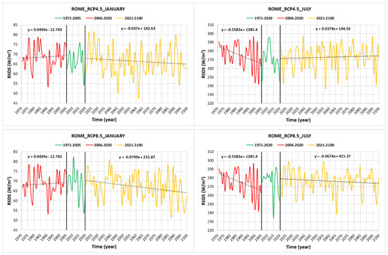
Figure 3.
Rome’s monthly average hourly RSDS variation in January (left) and July (right) from 1971 to 2100. (Top): RCP4.5, (bottom): RCP8.5.
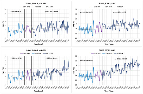
Figure 4.
Rome’s monthly average hourly TAS variation in January (left) and July (right) from 1971 to 2100. (Top): RCP4.5, (bottom): RCP8.5.
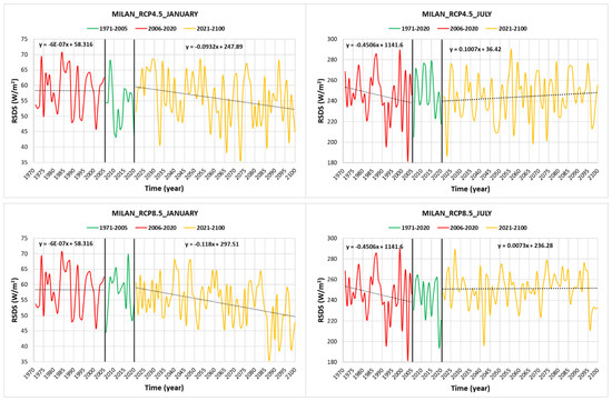
Figure 5.
Milan’s monthly average hourly RSDS variation in January (left) and July (right) from 1971 to 2100. (Top): RCP4.5, (bottom): RCP8.5.
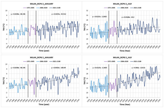
Figure 6.
Milan’s monthly average hourly TAS variation in January (left) and July (right) from 1971 to 2100. (Top): RCP4.5, (bottom): RCP8.5.
For Rome in January, RSDS has a slight average increasing trend in the past scenario, while it has an average decreasing trend in the future period, represented by the angular coefficient of the regression curve reported in the figures. This behaviour is highlighted both in the RCP4.5 and RCP8.5 scenarios. For the RCP8.5 scenario, the decrease rate is higher. Additionally, in July, there is a trend reversal for RSDS in the RCP4.5 scenario between the past and the future periods, which passes from an average decreasing trend to an increasing one; instead, it is decreasing in the RCP8.5 scenario but with a lower rate of decrease in the future period compared to the past period. For the TAS in January, all trends increase in all RCP scenarios and both in the past and future periods. Instead in July, for both RCP scenarios, TAS slightly decreases in the past scenario and increases in the future period. In the future scenario, a substantially higher rate of increase in the RCP8.5 scenarios is highlighted compared to one of the RCP4.5 scenarios.
For Milan in January, for all RCP scenarios, a rate of decrease in RSDS is observed for the future period. In the past scenario, the rate of decrease is not relevant, and the trend can be considered almost constant. Instead, in July for both RCP scenarios, a reversal is observed from the past period to the future period. In particular, an average decrease and an average increase are observed in the past and future periods, respectively. This reversal is more pronounced in the RCP4.5 scenario. For the TAS, all trends are increasing in the past and future periods for all RCP scenarios and months. Similarly to Rome, a substantially higher rate of increase in the RCP8.5 scenarios is highlighted compared to one of the RCP4.5 scenarios in Milan.
4.2. Photovoltaic Electricity Production Projection
The influence of climate change on the performance of the PV module considered was studied. The monthly energy PV produced in January and July, the yearly energy, and the yearly average PV efficiency were calculated in all cases considered and reported in Figure 7 and Figure 8 for Rome and Figure 9 and Figure 10 for Milan.
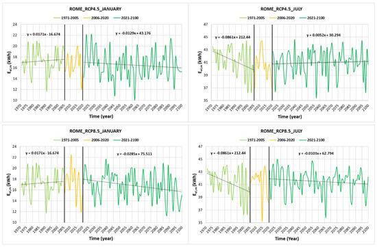
Figure 7.
Rome’s monthly PV electricity variation in January (left) and July (right) from 1971 to 2100. (Top): RCP4.5, (bottom): RCP8.5.
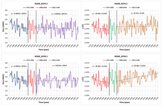
Figure 8.
Rome’s yearly PV electricity variation (left) and yearly PV efficiency variation (right) from 1971 to 2100. (Top): RCP4.5, (bottom): RCP8.5.
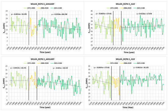
Figure 9.
Milan’s monthly PV electricity variation in January (left) and July (right) from 1971 to 2100. (Top): RCP4.5, (bottom): RCP8.5.
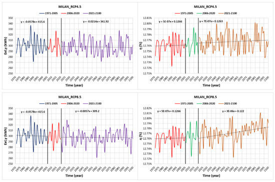
Figure 10.
Milan’s yearly PV electricity variation (left) and yearly PV efficiency variation (right) from 1971 to 2100. (Top): RCP4.5, (bottom): RCP8.5.
For Rome in January, a reversal is observed for the rate of increase of the monthly PV energy produced in the past and future periods for the RCP4.5 scenario, which are, respectively, 17.1 Wh/year and −12.9 Wh/year; instead; the rate of increase changes substantially from 17.1 Wh/year to −28.5 Wh/year in the RCP8.5 scenario. In July, the rate of increase of the monthly PV energy produced undergoes a reversal from −86.1 Wh/year to 5.2 Wh/year in the RCP4.5 scenario, while it is equal to −86.1 Wh/year in the past scenario and 10.3 Wh/year in the future period in the RCP8.5 scenario. In Rome, the rate of increase of yearly PV energy produced substantially changes from −369.5 Wh/year to −50.5 Wh/year in the RCP4.5 scenario and from −369.5 Wh/year to −11.1 Wh/year in the RCP8.5 scenario. This means that the reduction in the yearly energy produced observed in the past period will be less significant in the future period for both RCP scenarios. As regards the yearly PV efficiency, no relevant changes can be detected in both RCP scenarios with only an average increase of 0.02% in 80 years from 2021 to 2100 in the high emissions scenario RCP8.5. This result can be associated with the strong dependence of the reference PV efficiency on the PV module characteristics and materials that are the same in all scenarios considered; instead, the temperature and solar radiation do not significantly affect the yearly average PV efficiency and mainly influence the instantaneous PV efficiency. This can be explained by considering that there is a compensative effect on instantaneous variations of the PV efficiency during the year. Finally, changes in efficiency from 12.83% to 12.85% cannot be considered statistically significant due to uncertainties in climate change models.
For Milan in January, the rates of increase of the monthly PV energy produced in the past and future periods are, respectively, −1.4 Wh/year and −35.8 Wh/year in the RCP4.5 scenario and −1.4 Wh/year and −43.0 Wh/year. In July, the rate of increase of the monthly PV energy produced undergoes a reversal from −68.3 Wh/year to 15.6 Wh/year in the RCP4.5 scenario, while it is equal to −68.3 Wh/year in the past scenario and 1.3 Wh/year in the future period. In Milan, the rate of increase of yearly PV energy produced changes from −57.8 Wh/year to −21.4 Wh/year in the RCP4.5 scenario and from −57.8 Wh/year to −5.7 Wh/year in the RCP8.5 scenario. This means that also in Milan, the reduction in the yearly energy produced observed in the past period will be less significant in the future period for both RCP scenarios. As regards the yearly average PV efficiency, analogous consideration performed for Rome can be extended to Milan.
5. Conclusions
A climate projection dataset has been produced for use in the PV sector. This dataset features a high spatial and temporal resolution in line with energy needs and a multi-scenario ensemble to account for uncertainties in climate projections. Specifically, in the present study, projected climate changes were examined in two Italian localities (Rome and Milan) considering high-resolution simulations provided by the EURO-CORDEX project under the RCP4.5 and RCP8.5 scenarios. Two climate variables (TAS and RSDS) were evaluated for the past (1971–2020) and future (2021–2100) periods.
Among 38 GCM-RCM models, the CCLM 4-8-17—EC EARTH was chosen since it provides intermediate values of climate variables (TAS and RSDS) among all models. This choice was fundamental to reduce the huge dataset that for only one model, one variable, and two RCP scenarios, the monthly average hourly data for 1971–2100 for Europe is about 6 Gb.
Through the climatic data and the use of TRNSYS software, it was possible to obtain the data on electrical energy produced by a single PV module characterized by a nominal power of 250.22 W. The results demonstrated that climate changes have influenced PV energy production in the past period and will continue to cause a reduction in energy production. Based on the obtained results, the reduction in the yearly produced energy observed in the past period will be less significant in the future period for both RCP scenarios and localities. The rates of decrease calculated in the past period in both localities and RCP scenarios are found to be higher than those obtained in the future period. In particular, in the stabilization RCP4.5 scenario, the PV energy per rated power, namely, the ratio of the energy yield to the peak power of the PV module, will be reduced on average by 0.202 Wh/W per year in Rome and by 0.086 Wh/W per year in Milan in the future period. Instead, in the high emissions RCP8.5 scenario, it will be reduced on average by 0.044 Wh/W per year in Rome and by 0.023 Wh/W per year in Milan in the future period. The corresponding values in the past period are 1.477 Wh/W per year in Rome and 0.231 Wh/W per year in Milan. Consequently, an overall almost constant trend is expected in the future period. This small positive effect of climate change on PV energy production depends only on the changes in the climate variables in the coming years, which, on the other hand, has very little influence on PV efficiency, which is an intrinsic parameter of the PV cell.
Ultimately, it can be argued that climate change is unlikely to compromise the Italian development of the PV sector. Instead, considering the forecasts found together with the slight improvement in the PV performance and reduction in the PV purchase costs foreseen in the coming years, the PV market in Italy will considerably grow.
Author Contributions
Conceptualization, N.M. and D.M.; methodology, N.M. and D.M.; software, N.M. and D.M.; validation, C.B. and P.M.C.; formal analysis, D.M. and P.M.C.; investigation, N.M. and C.B.; resources, N.M. and P.M.C.; data curation, N.M. and D.M.; writing—original draft preparation, D.M. and N.M.; writing—review and editing, N.M., D.M., C.B. and P.M.C.; visualization, N.M., D.M., C.B. and P.M.C. All authors have read and agreed to the published version of the manuscript.
Funding
This research received no external funding.
Institutional Review Board Statement
Not applicable.
Informed Consent Statement
Not applicable.
Data Availability Statement
Not applicable.
Conflicts of Interest
The authors declare no conflict of interest.
Nomenclature
| A | Area of the PV module | m2 |
| AR5 | Fifth Assessment Report | |
| CMIP5 | Coupled Model Intercomparison Project Phase 5 | |
| Eel,m | Monthly electrical energy produced in one month | Wh |
| Eel,y | Yearly electrical energy produced in one month | Wh |
| GCM | Global climate model | |
| Gy | Yearly solar radiation incident on the inclined plane | Wh/m2 |
| Imp | Current at the point of maximum power | A |
| IPCC | Intergovernmental Panel on Climate Change | |
| Isc | Short circuit current at reference conditions | A |
| NOCT | Nominal operating cell temperature | K |
| PV | Photovoltaic | |
| RCM | Regional Climate Model | |
| RCP | Representative Concentration Pathway scenario | |
| RF | Total radiative forcing (energy absorbed − energy emitted) | W/m2 |
| RSDS | Surface downwelling shortwave radiation | W/m2 |
| TAS | Near-surface air temperature (TAS) | |
| Vmp | Voltage at the point of maximum power | V |
| Voc | Open circuit voltage at reference conditions | V |
| η | Yearly photovoltaic efficiency |
References
- European Commission. Communication from the Commission to the European Parliament, the European Council, the Council, the European Economic and Social Committee, the Committee of the Regions and the European Investment Bank a Clean Planet for All a European Strategic Long-Term; European Commission: Brussels, Belgium, 2018. [Google Scholar]
- Mazzeo, D.; Matera, N.; De Luca, P.; Baglivo, C.; Congedo, P.M.; Oliveti, G. Worldwide geographical mapping and optimization of stand-alone and grid-connected hybrid renewable system techno-economic performance across Köppen-Geiger climates. Appl. Energy 2020, 276, 115507. [Google Scholar] [CrossRef]
- Russo, M.A.; Carvalho, D.; Martins, N.; Monteiro, A. Forecasting the inevitable: A review on the impacts of climate change on renewable energy resources. Sustain. Energy Technol. Assess. 2022, 52, 102283. [Google Scholar] [CrossRef]
- Kandeal, A.W.; Thakur, A.K.; Elkadeem, M.R.; Elmorshedy, M.F.; Ullah, Z.; Sathyamurthy, R.; Sharshir, S.W. Photovoltaics performance improvement using different cooling methodologies: A state-of-art review. J. Clean. Prod. 2020, 273, 122772. [Google Scholar] [CrossRef]
- Dehghan, M.; Rahgozar, S.; Pourrajabian, A.; Aminy, M.; Halek, F.S. Techno-economic perspectives of the temperature management of photovoltaic (PV) power plants: A case-study in Iran. Sustain. Energy Technol. Assess. 2021, 45, 101133. [Google Scholar] [CrossRef]
- Dehghan, M.; Rashidi, S.; Waqas, A. Modeling of soiling losses in solar energy systems. Sustain. Energy Technol. Assess. 2022, 53, 102435. [Google Scholar] [CrossRef]
- Intergovernmental Panel on Climate Change (IPCC), Geneva (Switzerland). Available online: https://www.ipcc.ch (accessed on 4 February 2022).
- Hoegh-Guldberg, O.; Jacob, D.; Taylor, M.A.; Bindi, M.; Brown, S.; Camilloni, I.; Diedhiou, A.; Djalante, R.; Ebi, K.L.; Engelbrecht, F.; et al. Impacts of 1.5 °C Global Warming on Natural and Human Systems. In Global Warming of 1.5 °C. An IPCC Special Report on the Impacts of Global Warming of 1.5 °C above Pre-Industrial Levels and Related Global Greenhouse Gas Emission Pathways, in the Context of Strengthening the Global Response to the Threat of Climate Change, Sustainable Development, and Efforts to Eradicate Poverty; Masson-Delmotte, V., Zhai, P., Pörtner, H.O., Roberts, D., Skea, J., Shukla, P.R., Pirani, A., Moufouma-Okia, W., Péan, C., Pidcock, R., et al., Eds.; Cambridge University Press: Cambridge, UK, 2018; in press. [Google Scholar]
- IPCC. Climate Change 2014: Synthesis Report. Contribution of Working Groups I, II and III to the Fifth Assessment Report of the Intergovernmental Panel on Climate Change; IPCC: Geneva, Switzerland, 2014; p. 151. Available online: https://www.ipcc.ch/report/ar5/syr/ (accessed on 20 October 2022).
- Tettey, U.Y.A.; Gustavsson, L. Energy savings and overheating risk of deep energy renovation of a multi-storey residential building in a cold climate under climate change. Energy 2020, 202, 117578. [Google Scholar] [CrossRef]
- Muñoz González, C.M.; León Rodríguez, A.L.; Suárez Medina, R.; Ruiz Jaramillo, J. Effects of future climate change on the preservation of artworks, thermal comfort and energy consumption in historic buildings. Appl. Energy 2020, 276, 115483. [Google Scholar] [CrossRef]
- Malvoni, M.; Leggieri, A.; Maggiotto, G.; Congedo, P.M.; De Giorgi, M.G. Long term performance, losses and efficiency analysis of a 960 kWP photovoltaic system in the Mediterranean climate. Energy Convers. Manag. 2017, 145, 169–181. [Google Scholar] [CrossRef]
- Peters, M.; Buonassisi, T. The Impact of Global Warming on Silicon PV Energy Yield in 2100. In Proceedings of the 2019 IEEE 46th Photovoltaic Specialists Conference (PVSC), Chicago, IL, USA, 16–21 June 2019; pp. 3179–3181. [Google Scholar] [CrossRef]
- Crook, J.A.; Jones, L.A.; Forster, P.M.; Crook, R. Climate change impacts on future photovoltaic and concentrated solar power energy output. Energy Environ. Sci. 2011, 4, 3101–3109. [Google Scholar] [CrossRef]
- Wild, M.; Folini, D.; Henschel, F.; Fischer, N.; Müller, B. Projections of long-term changes in solar radiation based on CMIP5 climate models and their influence on energy yields of photovoltaic systems. Solar Energy 2015, 116, 12–24. [Google Scholar] [CrossRef]
- Nakićenović, N.; Swart, R. Special Report on Emissions Scenarios: A Special Report of Working Group III of the Intergovernmental Panel on Climate Change; Cambridge University Press: Cambridge, UK, 2000. [Google Scholar]
- Panagea, I.S.; Tsanis, I.K.; Koutroulis, A.G.; Grillakis, M.G. Climate change impact on photovoltaic energy output: The case of Greece. Adv. Meteorol. 2014, 2014, 264506. [Google Scholar] [CrossRef]
- Solomon, S.; Qin, D.; Manning, M.; Marquis, M.; Chen, Z.; Avery, K.B.; Tignor, M.; Miller, H.L. Climate Change 2007: The Physical Science Basis. In Contribution of Working Group I to the Fourth Assessment Report of the Intergovernmental Panel on Climate Change; Cambridge University Press: Cambridge, UK, 2007. [Google Scholar]
- Rummukainen, M. State-of-the-art with regional climate models. Wiley Interdiscip. Rev. Clim. Chang. 2010, 1, 82–96. [Google Scholar] [CrossRef]
- Gaur, A.; Simonovic, S.P. Chapter 4-Introduction to Physical Scaling: A Model Aimed to Bridge the Gap Between Statistical and Dynamic Downscaling Approaches; Teegavarapu, R., Ed.; Trends and Changes in Hydroclimatic Variables; Elsevier: Amsterdam, The Netherlands, 2019; pp. 199–273. [Google Scholar] [CrossRef]
- Hennemuth, T.I.; Jacob, D.; Keup-Thiel, E.; Kotlarski, S.; Nikulin, G.; Otto, J.; Szépszó, G. Guidance for EURO-CORDEX Climate Projections Data Use; Version 1.1. 2021. Available online: https://www.euro-cordex.net/imperia/md/content/csc/cordex/guidance_for_euro-cordex_climate_projections_data_use__2021-02_1_.pdf (accessed on 20 October 2022).
- Sørland, S.L.; Brogli, R.; Pothapakula, P.K.; Russo, E.; de Walle, J.V.; Ahrens, B.; Anders, I.; Bucchignani, E.; Davin, E.L.; Demory, M.-E.; et al. COSMO-CLM regional climate simulations in the Coordinated Regional Climate Downscaling Experiment (CORDEX) framework: A review. Geosci. Model. Dev. 2021, 14, 5125–5154. [Google Scholar] [CrossRef]
- Cinquini, L.; Crichton, D.; Mattmann, C.; Harney, J.; Shipman, G.; Wang, F.; Schweitzer, R. The Earth System Grid Federation: An open infrastructure for access to distributed geospatial data. Future Gener. Comput. Syst. 2014, 36, 400–417. [Google Scholar] [CrossRef]
- Congedo, P.M.; Baglivo, C.; Seyhan, A.K.; Marchetti, R. Worldwide dynamic predictive analysis of building performance under long-term climate change conditions. J. Build. Eng. 2021, 42, 103057. [Google Scholar] [CrossRef]
- Mazzeo, D.; Matera, N.; Bevilacqua, P.; Arcuri, N. Energy and economic analysis of solar photovoltaic plants located at the University of Calabria. Int. J. Heat Technol. 2015, 33, 41–50. [Google Scholar] [CrossRef]
- Herdem, M.S.; Mazzeo, D.; Matera, N.; Wen, J.Z.; Nathwani, J.; Hong, Z. Simulation and modeling of a combined biomass gasification-solar photovoltaic hydrogen production system for methanol synthesis via carbon dioxide hydrogenation. Energy Convers. Manag. 2020, 219, 113045. [Google Scholar] [CrossRef]
- Mazzeo, D. Nocturnal electric vehicle charging interacting with a residential photovoltaic-battery system: A 3E (energy, economic and environmental) analysis. Energy 2019, 168, 310–331. [Google Scholar] [CrossRef]
- Mazzeo, D. Solar and wind assisted heat pump to meet the building air conditioning and electric energy demand in the presence of an electric vehicle charging station and battery storage. J. Clean. Prod. 2019, 213, 1228–1250. [Google Scholar] [CrossRef]
- Solar Energy Laboratory, University of Wisconsin-Madison, TRNSYS 17 Documentation, Volume 4, Mathematical Reference. 2012. Available online: https://www.trnsys.com (accessed on 20 October 2022).
- Jakson Group, Noida Uttar Pradesh, India. Available online: https://www.jakson.com (accessed on 20 October 2022).
Publisher’s Note: MDPI stays neutral with regard to jurisdictional claims in published maps and institutional affiliations. |
© 2022 by the authors. Licensee MDPI, Basel, Switzerland. This article is an open access article distributed under the terms and conditions of the Creative Commons Attribution (CC BY) license (https://creativecommons.org/licenses/by/4.0/).