Parameter Identification of Variable Flux Reluctance Machines Excited by Zero-Sequence Current Accounting for Inverter Nonlinearity

Abstract

To identify the parameters of variable flux reluctance machines (VFRMs), the input voltage value is usually obtained from the reference voltage indirectly. However, the reference and actual voltages may be different due to the nonlinearity of the open winding inverter when using zero-sequence current, leading to the inaccuracy of parameter identification. To solve this problem, this paper proposes an equivalent nonlinearity voltage error model of the open winding inverter to compensate for the input voltage of VFRM during the online parameter identification. Since in the proposed method the phase current direction is not required, the calculation time can be reduced. Moreover, in the developed parameter identification model of VFRM the derived equivalent nonlinear voltage error is used to correct the input of the identification model so as to improve the accuracy of parameters. Finally, the experimental results on the prototype VFRM are presented for verification.

1. Introduction

Variable flux reluctance machines (VFRMs) are brushless synchronous machines with stator excitation [1], with no winding or a permanent magnet on the rotor. VFRMs have good application prospects for their excellent heat dissipation performance, wide speed range, stable performance, and low cost [2,3]. In the control of VFRMs, integrated excitation and armature windings are used, in which the stator currents contain AC components and DC (zero-sequence) components. The AC component of the stator current acts as the armature current, and the zero-sequence component acts as the excitation current [4,5]. To provide a loop for zero-sequence current, an open winding inverter with a common DC bus is used [6,7].

Online parameter identification is essential for high-performance machine control, such as flux-weakening control, controller tuning, and sensorless control [8,9,10,11,12]. Online parameter identification methods, including the recursive least squares method [8], model reference adaptation [13], and Kalman filter algorithm [14], have been used for permanent magnet synchronous machines (PMSMs) and induction machines. In online parameter identification, it is necessary to obtain the terminal voltage of machines in real-time. However, voltage sensors will increase the control system’s cost and complexity, which is unsuitable for low-cost applications. Therefore, a promising way to obtain the terminal voltage from the reference voltage is the parameter identification. However, due to the inverter nonlinearity, there is a difference between the reference voltage and the terminal voltage, which would result in inaccurate parameter identification results. The nonlinearity of the inverter is mainly due to the dead time, the voltage drop of power devices, and the error of DC bus voltage. The dead time is set in the program to prevent the two power devices of the same inverter leg from being turned on simultaneously. However, the dead time distorts the output voltage of the inverter [15]. On the other hand, the power device is not ideal. During conduction (e.g., IGBT) and freewheeling (e.g., diode), there is the saturation voltage drop, which distorts the inverter output voltage. Since the duty cycle in PWM modulation is related to the DC bus voltage, the inverter nonlinearity can also be caused by DC bus voltage error [16]. Especially when the open winding inverter is used in VFRM, the inverter nonlinearity is twice that of the single inverter. Moreover, in VFRM with zero-sequence current excitation, the direction of the stator current is not changing every 180 degrees due to the DC component, which is different from the stator current in PMSM. Thus, the presence of zero-sequence current in the stator current increases the complexity of the inverter nonlinearity. Therefore, to increase the accuracy of VFRM parameter identification, it is necessary to study the nonlinearity of the open-winding inverter using zero-sequence current excitation.

To suppress the influence of inverter nonlinearity on parameter identification, an online dead time compensation method was proposed in [15], in which the nonlinearity caused by the dead time effect is compensated for, but the voltage drops of power devices are not discussed. To achieve the nonlinearity compensation, the model reference adaptive method is used in [16] to estimate the variables that need to be compensated for for inverter nonlinearity. In [17], the influence of inverter nonlinearity on parameter identification is analyzed. The aforementioned methods focus on the nonlinearity compensation of a single inverter. Some literature [18] has analyzed the nonlinearity of a dual inverter for dual three-phase IPMSM, but the nonlinearity in zero-sequence is not mentioned. Zero-sequence voltage is used to compensate for the dead-time in an open winding inverter in [19]. In VFRM, however, zero-sequence voltage cannot be used in nonlinearity compensation since it is used to control the excitation current. A closed loop nonlinearity compensation method for an open winding inverter is proposed in [20], which requires several electrical periods to converge when a step current is applied.

Therefore, the previous work focuses on the inverter nonlinearity compensation other than the voltage error due to the nonlinearity, which is required for the actual voltage without voltage sensors. In VFRM with zero-sequence current excitation, the current direction is not changing every 180-degree due to the DC component. Additionally, the harmonics in the back-EMF of the VFRM and the inverter nonlinearity result in high current harmonics [21]. Therefore, the traditional inverter nonlinearity compensation methods cannot effectively reduce the current distortion. In this case, the current distortion caused by back-EMF harmonics and inverter nonlinearity are both suppressed by the specified order harmonic suppression algorithm [22]. Since the inverter nonlinearity is also compensated for by the harmonic suppression algorithm, to obtain the actual voltage, the equivalent dq0-axis voltage error caused by the open winding inverter nonlinearity should be investigated.

In this paper, by analyzing the operating characteristics of the open winding, the equivalent nonlinearity model of open winding inverter for VFRM using zero-sequence current excitation is proposed. The model does not need the direction of phase current, resulting in lower calculation burden. The parameter identification of VFRM with high accuracy is developed by using the recursive least square method, and the identification of resistance and inductance is realized by the reference voltage with nonlinear inverter voltage error compensation. Finally, the parameter identification method accounting for the nonlinearity model of VFRM is verified by experiments.

2. Control and Parameter Identification of VFRM

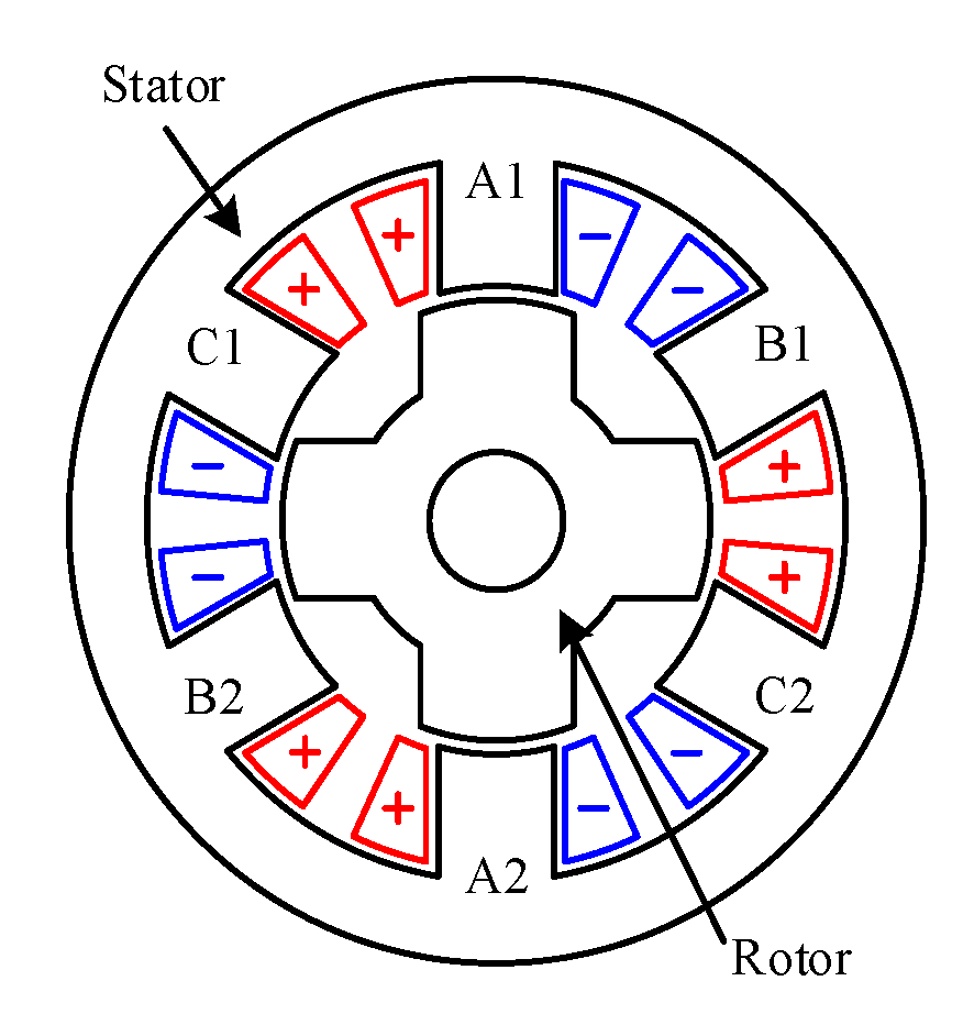
2.1. Model of VFRM

The topology of a 6/4 VFRM is shown in Figure 1. In the windings of VFRM, the stator currents contain varying and constant components, in which the varying current component acts as armature current and the constant component acts as excitation current. To provide the loop for zero-sequence current, the open winding inverter with a common DC bus is used in the driving system, as shown in Figure 2. The expressions of stator currents are

$$\{\begin{array}{l}{i}_a=I_{AC}\cos \left({\omega }_{e}t\right)+I_{DC}\\ i_b=I_{AC}\cos \left({\omega }_{e}t-2\pi /3\right)+I_{DC}\\ i_c=I_{AC}\cos \left({\omega }_{e}t+2\pi /3\right)+I_{DC}\end{array}$$

(1)

where i_a, i_b, i_c are the stator currents, I_AC is the amplitude of the varying current component, and I_DC is the zero-sequence component (will be replaced with i₀ below). ω_e is the electrical angular velocity.

The voltage equation of 6/4 VFRM is shown in (2), where the third-order component voltages are included. The third-order harmonics in the dq-plane are the map of second-order harmonics in the fundamental component [5].

$$\left[\begin{array}{c}{u}_d\\ u_q\\ u_0\end{array}\right]=R_s\left[\begin{array}{c}{i}_d\\ i_q\\ i_0\end{array}\right]+{\omega }_e\left[\begin{array}{ccc}-L_{\delta }\sin 3{\theta }_e& -L_s-L_{\delta }\cos 3{\theta }_e& 0\\ L_s-L_{\delta }\cos 3{\theta }_e& L_{\delta }\sin 3{\theta }_e& L_{\delta }\\ 0& 0& 0\end{array}\right]\left[\begin{array}{c}{i}_d\\ i_q\\ i_0\end{array}\right]$$

(2)

where u_d, u_q, and u₀ are the d-, q- and 0-axis voltage components, R_s is the resistance of winding, L_s is the constant component of stator winding inductance, and L_δ is the alternating component of stator winding inductance. θ_e is the electrical angle.

Since the harmonics in the back-EMF of VFRM and inverter nonlinearity can cause current distortion, the specific order harmonics compensation algorithm [21] is used to eliminate the current harmonics. The basic principle of the specific order harmonics compensation algorithm is to extract the dq component of the harmonic component to be suppressed using different orders of the dq transform, since the other harmonics will produce harmonics in the dq axis of the target order. Therefore, the target dq-axis components of the harmonic currents can be extracted using a low-pass filter. Finally, the harmonic current loop is constructed based on the extracted harmonic current dq components, and the given value is set to 0. After the current loop is stabilized, the harmonic is suppressed to 0.

2.2. Parameter Identification of VFRM

Since the voltage harmonics are compensated for, the voltage equations shown in (3) can be used in parameter identification. There are three parameters that need to be identified in (3): resistance R_s, inductances L_s and L_δ.

$$\{\begin{array}{l}{u}_d=R_s{i}_d-{\omega }_e{L}_s{i}_q\\ u_q=R_s{i}_q+{\omega }_e\left(L_s{i}_d+L_{\delta }{i}_0\right)\\ u_0=R_s{i}_0\end{array}$$

(3)

In the parameter identification of PMSM, the parameters that need to be identified are more than the degree of voltage equations, which results in rank deficiency. In this situation, the number of identified parameters should be limited, or a signal injection method is needed [18]. Nevertheless, in the parameter identification of VFRM, the voltage equations represent three independent algebraic equations. Therefore, the parameters of VFRM can be identified by using the recursive least squares method [8]. According to (3), the recursion equation of the parameter identification of VFRM is

$${\widehat{\theta }}_t={\widehat{\theta }}_{t-1}+P_k\left(x_k{y}_k-x_k{x}_k^T{\widehat{\theta }}_{t-1}\right)$$

(4)

where y_k is the vector of estimated variables, θ_t is the estimated parameter vector and ${\widehat{\theta }}_0=0$, P_k is the correction gain matrix and P₀ = αI, α is a positive real value, x_k is the regressor.

$$y_k=\left[\begin{array}{l}{R}_s{i}_d-{\omega }_e{L}_s{i}_q\\ R_s{i}_q+{\omega }_e\left(L_s{i}_d+L_{\delta }{i}_0\right)\\ R_s{i}_0\end{array}\right]=\left[\begin{array}{c}{u}_d\\ u_q\\ u_0\end{array}\right]$$

(5)

$$x_k=\left[\begin{array}{ccc}{i}_d& -{\omega }_e{i}_q& 0\\ i_q& {\omega }_e{i}_d& {\omega }_e{i}_0\\ i_0& 0& 0\end{array}\right]$$

(6)

$$\widehat{\theta }={\left[\begin{array}{ccc}{R}_s& L_s& L_{\delta }\end{array}\right]}^T$$

(7)

$$P_k=P_{k-1}-P_{k-1}{x}_k{\left[I+x_k^T{P}_{k-1}{x}_k\right]}^{-1}{x}_k^T{P}_{k-1}$$

(8)

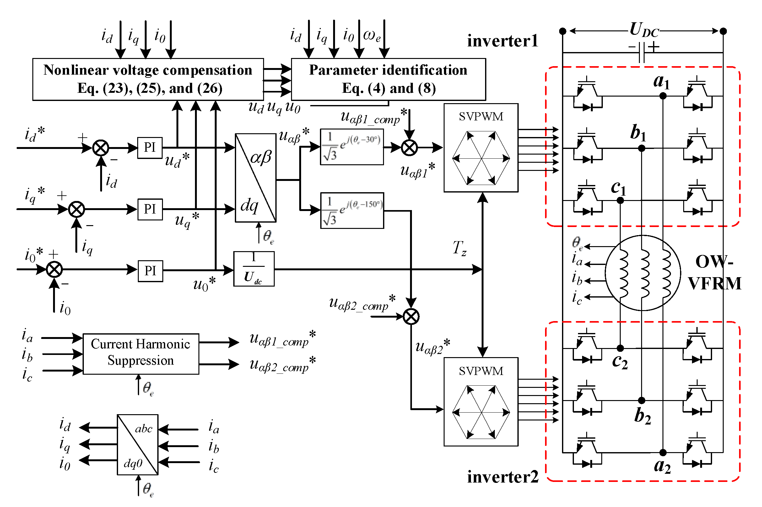
3. Nonlinearity of Open Winding Inverter and Its Compensation

The actual voltage of VFRM is required in parameter identification. However, the actual voltage is often obtained indirectly from the reference voltage to reduce the cost. Since the reference voltage and actual voltage are different, the investigation of open winding nonlinearity is necessary to improve the accuracy of VFRM parameter identification.

In this section, the nonlinear mathematical model of the open winding inverter is developed based on different power device states and current directions.

3.1. Analysis of Three-Phase Nonlinear Voltage

Taking one phase bridge leg and winding as an example, in Figure 3, the current flows forward from inverter 1 to inverter 2. In Figure 3a, when the S11 is turned on and S21 turned off, the current flows through S11 and S22, so the terminal voltage of winding A (V_a) equals the supply voltage minus the voltage drop of the two active switches. When S21 is turned on, the current freewheels through S11 and D21. V_a equals the negative values of voltage drops of S11 and D21. In Figure 3b, S11 and S21 are turned off, and the current freewheels through D12 and S22; V_a equals the negative value of voltage drops of D12 and S22 at this time. When S21 turns on, the current passes through D21 and D22, V_a equals the supply voltage minus the voltage drop of two diodes. The analysis is similar when the current flows in the opposite direction, as shown in Figure 3c,d. All the results of these cases are shown in

Table 1. Actual voltage in different switching states.

Current Direction	Switching State	S11 = 1	S11 = 0
ia > 0	S21 = 1	$V_a=-V_{ce}-V_d$	$V_a=-V_{DC}-2V_d$
	S21 = 0	$V_a=V_{DC}-2V_{ce}$	$V_a=-V_{ce}-V_d$
ia < 0	S21 = 1	$V_a=V_{ce}+V_d$	$V_a=-V_{DC}+2V_{ce}$
	S21 = 0	$V_a=V_{DC}+2V_d$	$V_a=V_{ce}+V_d$

Where V_DC is the DC-link voltage, V_ce and V_d are the voltage drop of the active switch and freewheeling diode, respectively.

.

Based on the above cases, the terminal voltages of phase A winding can be obtained as (9).

$$V_a=\left(V_{DC}-V_{ce}+V_d\right)\frac{T_a}{T_s}+\mathrm{sgn}\left(i_a\right)\left(V_{ce}+V_d\right)$$

(9)

where T_a is the equivalent on-time of a switching period. T_s is the switching period.

Since there are two inverters in series, as shown in Figure 2, the symmetrical modulation of the two inverters doubles the time error effect (mainly dead-time effect). The on-time should be calculated by Equation (10) [9]

$$T_a=\left(T_{a1}^{\ast }-T_{a2}^{\ast }\right)-2\mathrm{sgn}\left(i_a\right)t_{com}$$

(10)

where $T_{a1}^{*}$ and $T_{a2}^{*}$ are the on-time in a switching period of two inverters, respectively. t_com = t_d + t_–n − t_off is the total time error, in which t_d is the dead time, t_on is the sum of turn-on delay and turn-on transition time, and t_off is the sum of turn-off delay and turn-off transition time.

Therefore, the three-phase voltage after considering the device voltage drop and dead time can be expressed by:

$$\left[\begin{array}{c}{V}_a\\ V_b\\ V_c\end{array}\right]=\frac{V_{DC}-V_{nl1}}{T_s}\left[\begin{array}{c}{T}_a^{\ast }\\ T_b^{\ast }\\ T_c^{\ast }\end{array}\right]-\left[\left(V_{DC}-V_{nl1}\right)\frac{t_{com}}{T_s}+V_{nl2}\right]\left[\begin{array}{c}\mathrm{sgn}\left(i_a\right)\\ \mathrm{sgn}\left(i_b\right)\\ \mathrm{sgn}\left(i_c\right)\end{array}\right]$$

(11)

where

$$\{\begin{array}{l}{V}_{nl1}=V_{ce}-V_d\\ V_{nl2}=V_{ce}+V_d\end{array}$$

(12)

The difference between the reference voltages and actual voltages can be written as:

$$\left[\begin{array}{c}{V}_{aerr}\\ V_{berr}\\ V_{cerr}\end{array}\right]=\left[\begin{array}{c}{V}_a^{\ast }\\ V_b^{\ast }\\ V_c^{\ast }\end{array}\right]-\left[\begin{array}{c}{V}_a\\ V_b\\ V_c\end{array}\right]=V_{nl1}\left[\begin{array}{c}{T}_a^{\ast }/T_s\\ T_b^{\ast }/T_s\\ T_c^{\ast }/T_s\end{array}\right]+\left[\left(V_{DC}-V_{nl1}\right)\frac{t_{com}}{T_s}+V_{nl2}\right]\left[\begin{array}{c}\mathrm{sgn}\left(i_a\right)\\ \mathrm{sgn}\left(i_b\right)\\ \mathrm{sgn}\left(i_c\right)\end{array}\right]$$

(13)

A stable DC power is used to provide power in the experiments, which is hardly affected by the load, so the change of DC bus voltage is ignored.

3.2. Analysis of d-, q-, and 0-Axis Nonlinear Voltage

According to (13), the dq0-axis voltage error caused by inverter nonlinearity can be obtained as

$$\left[\begin{array}{c}{V}_{derr}\\ V_{qerr}\\ V_{0err}\end{array}\right]=V_{nl1}{C}_{park}\left[\begin{array}{c}{T}_a^{\ast }/T_s\\ T_b^{\ast }/T_s\\ T_c^{\ast }/T_s\end{array}\right]+\left[\left(V_{DC}-V_{nl1}\right)\frac{t_{com}}{T_s}+V_{nl2}\right]C_{park}\left[\begin{array}{c}\mathrm{sgn}\left(i_a\right)\\ \mathrm{sgn}\left(i_b\right)\\ \mathrm{sgn}\left(i_c\right)\end{array}\right]$$

(14)

where C_park is Park transform matrix.

The nonlinearity of the open winding inverter can be divided into two parts according to (14). The first part is related to the duty cycle ($T_a^{*}$/T_s), i.e.,

$$\left[\begin{array}{c}{V}_{derr1}\\ V_{qerr1}\\ V_{0err1}\end{array}\right]=V_{nl1}{C}_{park}\left[\begin{array}{c}{T}_a^{\ast }/T_s\\ T_b^{\ast }/T_s\\ T_c^{\ast }/T_s\end{array}\right]=V_{nl1}\left[\begin{array}{c}{V}_d^{\ast }/V_{DC}\\ V_q^{\ast }/V_{DC}\\ V_0^{\ast }/V_{DC}\end{array}\right]$$

(15)

$$\left[\begin{array}{c}{V}_{derr2}\\ V_{qerr2}\\ V_{0err2}\end{array}\right]=\left[\left(V_{DC}-V_{nl1}\right)\frac{t_{com}}{T_s}+V_{nl2}\right]C_{park}\left[\begin{array}{c}\mathrm{sgn}\left(i_a\right)\\ \mathrm{sgn}\left(i_b\right)\\ \mathrm{sgn}\left(i_c\right)\end{array}\right]$$

(16)

Equation (16) shows the variable components of nonlinear voltage. The harmonic suppression algorithm has compensated for the inverter nonlinearity. Accordingly, the equivalent voltage error needs to be calculated. It should be noted that the amplitude of V_nl1 and duty cycle is relatively small compared with the second part of inverter nonlinearity. Thus, the first part of nonlinearity can be neglected. For example, according to the parameters of IGBT, the amplitude of V_nl1 is about 0.6 V. When u₀ is 10 V and V_dc is 80 V, then the amplitude of V_0err1 is about 0.075 V. In the meantime, V_0err2 is about 4–5 V, which means the first part of nonlinearity is only 1% of the second part.

In the traditional method, the sign of phase current direction is used for inverter nonlinearity calculation, which increases the calculation time. Moreover, the current direction’s sign fluctuates around the zero-crossing point, resulting in clutter. Since the ratio of i₀ to the AC amplitude can affect the commutation angle of current, the relationship between nonlinear voltage and current direction is converted into the ratio of i₀ to the AC component. Thus, the calculation of the nonlinear voltage can be simplified. The expression for the second part of the dq0-axis nonlinear voltages can be written as:

$$\{\begin{array}{l}{V}_{derr2}=2A\left[\mathrm{sgn}\left(i_a\right)\cos {\theta }_e+\mathrm{sgn}\left(i_b\right)\cos \left({\theta }_e-\frac{2\pi }{3}\right)+\mathrm{sgn}\left(i_c\right)\cos \left({\theta }_e+\frac{2\pi }{3}\right)\right]\\ V_{qerr2}=-2A\left[\mathrm{sgn}\left(i_a\right)\sin {\theta }_e+\mathrm{sgn}\left(i_b\right)\sin \left({\theta }_e-\frac{2\pi }{3}\right)+\mathrm{sgn}\left(i_c\right)\cos \left({\theta }_e+\frac{2\pi }{3}\right)\right]\\ V_{0err2}=A\left[\mathrm{sgn}\left(i_a\right)+\mathrm{sgn}\left(i_b\right)+\mathrm{sgn}\left(i_c\right)\right]\end{array}$$

(17)

where A is the nonlinearity amplitude, i.e.,

$$A=\frac{1}{3}\left[\left(V_{DC}-V_{nl1}\right)\frac{t_{com}}{T_s}+V_{nl2}\right]$$

(18)

Figure 4 shows the diagram of d-axis nonlinear voltage. During each cycle, the d-axis nonlinear voltage periodically changes three times. Therefore, the equivalent value of the d-axis nonlinear voltage can be obtained by integrating the non-zero waveforms between α_a and α_b. α_a is the electrical angle corresponding to the reverse moment of the A-phase current. Therefore, in the calculation of α_a, the current vector angle and the proportion of i₀ in the AC component need to be considered. Equation (19) is the expression of α_a.

$${\alpha }_a=\arcsin \frac{i_0}{\sqrt{i_d^2+i_q^2}}-\mathrm{acrcos}\frac{i_d}{\sqrt{i_d^2+i_q^2}}+\frac{\pi }{2}$$

(19)

α_b is the angle when phase current changes from negative to positive. Therefore, α_b is

$${\alpha }_b={\alpha }_a+2\arccos \frac{i_0}{\sqrt{i_d^2+i_q^2}}$$

(20)

The angle while the phase A current is negative is

$${\alpha }_c=2\arccos \frac{i_0}{\sqrt{i_d^2+i_q^2}}$$

(21)

Thus, the equivalent value of the d-axis nonlinear voltage can be calculated as follows

$$V_{derr2}=\frac{3A}{\pi }{\displaystyle {\int }_{{\alpha }_a}^{{\alpha }_b}\left[-\cos {\theta }_e+\cos \left({\theta }_e-\frac{2}{3}\pi \right)+\cos \left({\theta }_e+\frac{2}{3}\pi \right)\right]d{\theta }_e}$$

(22)

Solving Formula (22), we get

$$V_{derr2}=-\frac{{6A\sin \theta |}_{{\alpha }_a}^{{\alpha }_b}}{\pi }=A\frac{6}{\pi }\left(\sin {\alpha }_a-\sin {\alpha }_b\right)$$

(23)

It should be noted that Figure 4 corresponds to the case that the d-axis current is negative, and the angle of the current vector is not 0. When i_d = 0, the d-axis equivalent nonlinearity voltage will be 0.

Figure 5 shows the waveform of the q-axis nonlinear voltage. The q-axis nonlinear voltage also varies three times in each electrical cycle. Therefore, the non-zero waveform integral between α_a and α_b can be calculated to obtain the equivalent value of the q-axis nonlinear voltage. As shown in Equation (24)

$$V_{qerr2}=-\frac{3A}{\pi }{\displaystyle {\int }_{{\alpha }_a}^{{\alpha }_b}\left[-\sin {\theta }_e+\sin \left({\theta }_e-\frac{2}{3}\pi \right)+\sin \left({\theta }_e+\frac{2}{3}\pi \right)\right]d{\theta }_e}$$

(24)

By solving (24), the following equation can be obtained.

$$V_{qerr2}=-\frac{{6A\cos \theta |}_{{\alpha }_a}^{{\alpha }_b}}{\pi }=A\frac{6}{\pi }\left(\cos {\alpha }_a-\cos {\alpha }_b\right)$$

(25)

Figure 6 shows the waveform of nonlinear voltage on 0-axis. The equivalent value of the 0-axis nonlinear voltage is related to α_c, as shown in (26).

$$V_{0err2}=3A\left(1-{\alpha }_c/\pi \right),0\le {\alpha }_c\le \pi$$

(26)

3.3. Nonlinearity Compensation in Parameter Identification

The parameters of the inverter are shown in

Table 2. Parameters of inverter.

Parameters	Value
Vce (Typical value)	2.6 V
Vd (Typical value)	3.2 V
Ton	15 ns
Toff	110 ns
td	2 μs
VDC	80 V

. The second part is dominant in the inverter nonlinearity. α_a, α_b, α_c are calculated from i_d, i_q, i_0. Thus, in the case of harmonic suppression, this method can restore the actual voltage through the reference voltage by using Equations (23), (25) and (26) for compensation, which can provide voltage information for parameter identification.

The control system diagram, including inverter nonlinearity compensation, harmonic suppression, and parameter identification, is shown in Figure 7. Firstly, the harmonic suppression module provides voltage compensation for the harmonic current. Then, the equivalent error caused by the inverter nonlinearity between the reference voltage and the actual voltage is calculated by the nonlinear voltage calculation module. Finally, the inductance and resistance parameters of the VFRM are obtained through the parameter identification module.

4. Experimental Results

The experiments are carried out on the VFRM with zero-sequence current excitation for verification. The parameters of the VFRM used in the experiments are shown in

Table 3. Parameters of VFRM.

Parameters	Value	Parameters	Value
Poles of stator, Ns	6	Vary component of stator inductance, Lδ	24 mH
Poles of rotor, Nr	4	Rated speed	1000 rpm
Phase resistance, Rs	3Ω	Rated torque	0.5 Nm
Constant component of stator inductance, Ls	30 mH	Maximum current, imax	2 A

. The photo of the experimental platform is shown in Figure 8. The controller used in the experiment is dSPACE 1202. The VFRM is driven by an open winding inverter. The experiment data are collected with a Yokogawa DL850W oscilloscope and dSPACE host.

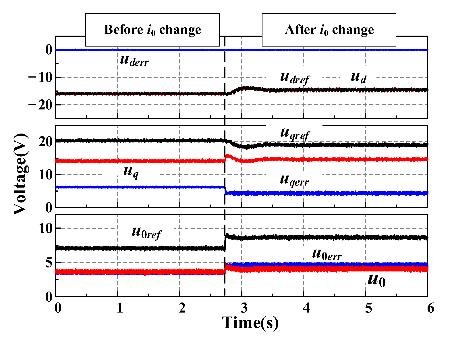
4.1. Inverter Nonlinear Verification

A three-phase balanced R-L load is used in the experiment to validate the proposed nonlinearity model. A regulated power supply powers the inverter in the experiment. The supply voltage is stable and does not affect the calculation of the nonlinear voltage. Figure 9 shows the measured voltage and the calculated voltage. The reference voltage values are u_d (−15 V), u_q (15 V), and u₀ (5 V), respectively. As in Figure 9, the voltages obtained by the two methods are in good agreement. Because of the influence of inverter nonlinearity, the actual values of u_d, u_q, and u₀ are smaller than their references in amplitude. Therefore, the correctness of the nonlinearity analysis of the inverter is verified.

The saturated voltage drop of the inverter devices will be affected by the operating conditions. Therefore, according to the datasheet of FGL40N120AND, the changes in parameters caused by different operational conditions are compensated for.

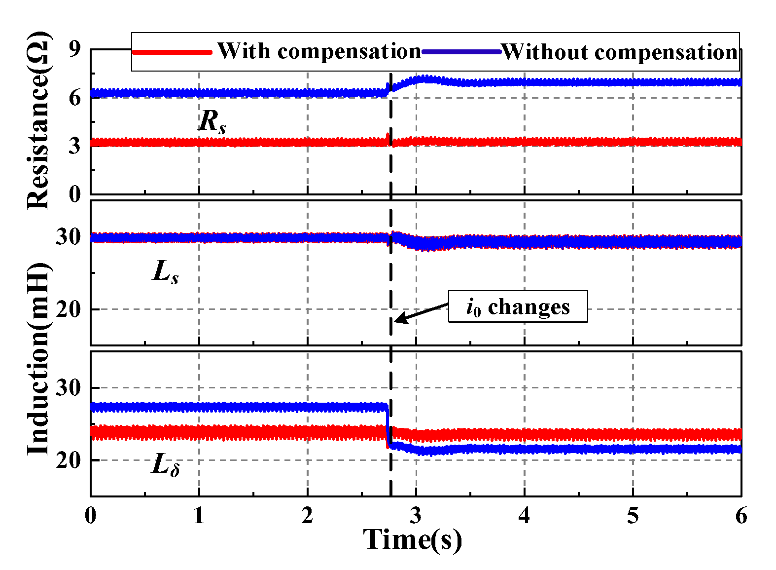
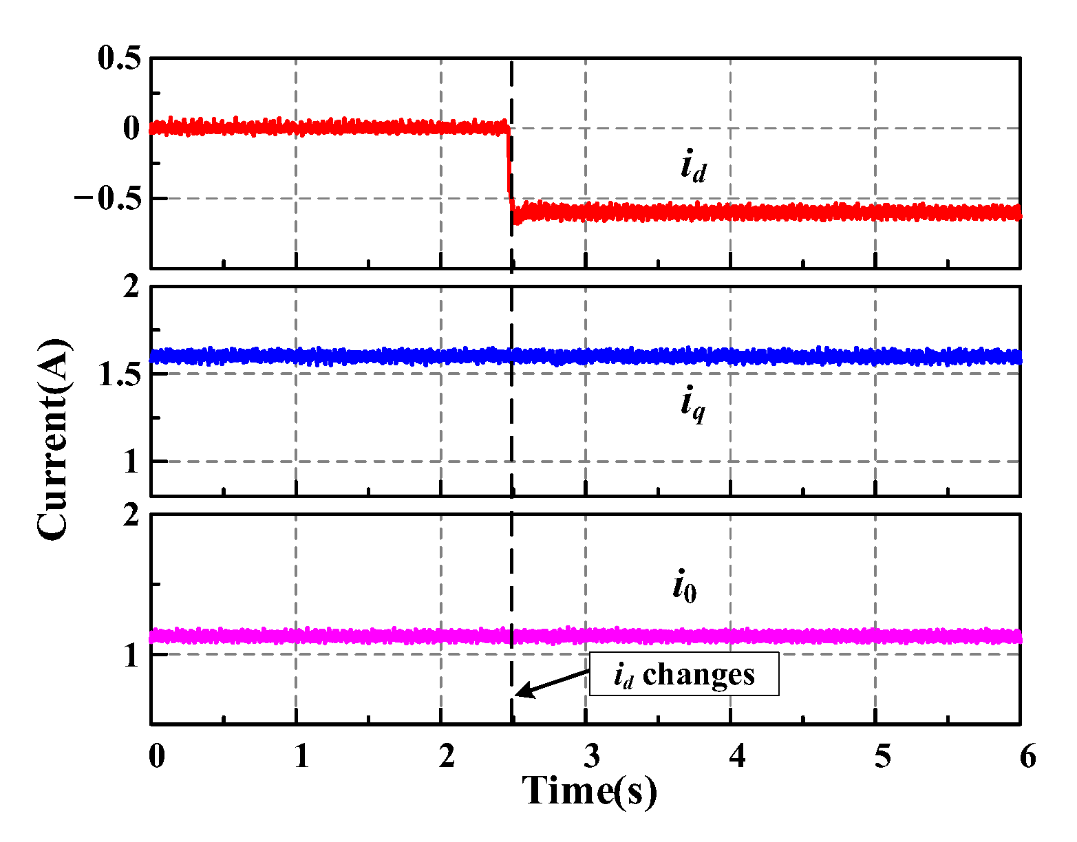
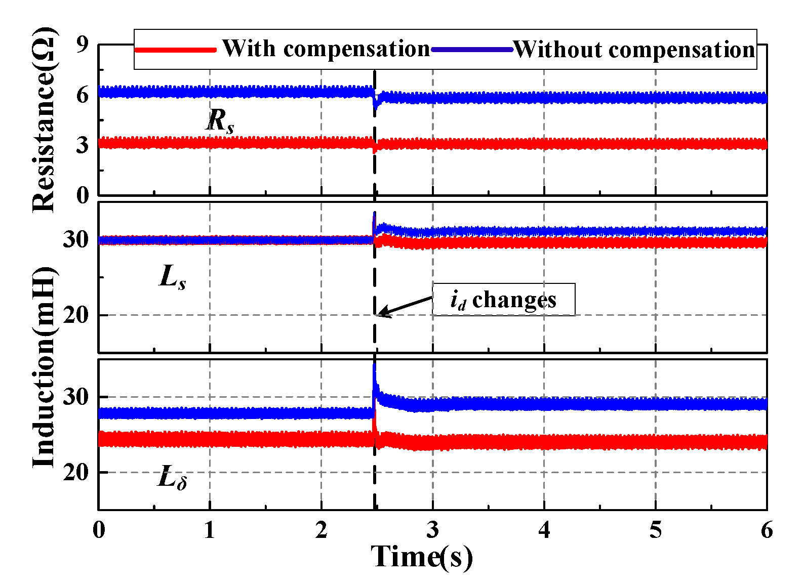
4.2. Influence of Inverter Nonlinearity on Parameter Identification

The experiments before and after the nonlinearity compensation are carried out to analyze the influence of inverter nonlinearity on parameter identification. Figure 10 shows the voltages before and after compensation. Before 3 s, the nonlinearity is not considered, and their values are 0. After 3 s, the inverter nonlinearity is calculated, and the reference voltage is compensated for to obtain the actual voltage. After compensation, the d-axis voltage does not change, and the q0-axis voltages decrease.

Figure 11 shows parameter identification results based on the voltages before and after nonlinearity compensation. When the reference voltage without compensation is used, there is a significant deviation between the parameter identification results and the nominal values in Table 3. Among them, R_s is twice of that without compensation, which are 6 Ω and 3 Ω. The error of R_s mainly comes from u_0err. Figure 10, the u_0err is close to u₀. Therefore, the nonlinearity causes R_s to be doubled before and after compensation according to (3). Moreover, L_s is only related to u_d, i_q, and ω_e when i_d is 0. Since the d-axis nonlinear voltage is 0, L_s does not change in Figure 12. L_δ is related to u_q. When u_q becomes smaller, L_δ also becomes closer to the nominal value.

The inverter nonlinearity can also be affected by i₀ and AC component ratio. A step increase of i₀ is implemented in the experiment to analyze this problem. Since the load torque remains unchanged, i_q decreases accordingly. Thus, the ratio between i₀ and the AC component becomes larger. Figure 12 shows the i_d, i_q, i₀, where i_d is 0. At about 2.7 s, i₀ increases.

Figure 13 shows the calculated nonlinear voltage and its equivalent value during i₀ changes. The zoomed waveforms after i₀ changes are also shown in Figure 13. After i₀ increases, V_0err increases, while i_q and V_qerr decrease. Since i_d remains 0, V_derr does not change. Figure 13 also shows the result of the nonlinear voltage passed through the low-pass filter. The filtered waveform is consistent with the calculated equivalent nonlinear voltage, which also verifies the accuracy of the proposed nonlinear voltage calculation method. However, the low-pass filter cannot be used in the nonlinear voltage calculation because of its computation burden and slow response speed.

The reference, actual, and equivalent nonlinear voltages during the dynamic process of i₀ are shown in Figure 14. After the step change of i₀, the equivalent nonlinearity of the 0-axis increases. Since i_q decreases, the nonlinearity of the q-axis becomes smaller. At the same time, the actual voltage also changes accordingly.

Parameter identification results while i₀ changes are shown in Figure 15. The identification results without nonlinearity compensation show a significant deviation. In comparison, the results with compensation are closer to the nominal value. For example, before and after the current changes, the identification accuracy of R_s is improved by about 106% and 123%. It should be noted that L_s has no deviation because the nonlinear voltage error on d-axis is 0. Therefore, the proposed method can improve the accuracy of parameter identification.

According to the analysis in Section 3, the change of i_d can affect the nonlinearity of an open winding inverter. To analyze this question, the reference of i_d is changed in the experiment. Figure 16 shows the current waveforms before and after i_d changes. i_d changes from 0 to −0.6 A around 2.4 s, while i_q and i₀ remain the same. Figure 17 shows the voltage waveforms during the change of i_d. More specifically, u_d and u_q decrease, while u₀ decreases slightly. Among them, the decrease of u_q is due to the change of i_d, and not to nonlinearity.

The parameter identification results during i_d changes are shown in Figure 18. The identification results without compensation show the deviation from the nominal value. The results with compensation are closer to the nominal value during the current changes. For instance, before and after the i_d changes, the identification accuracy of L_δ is improved by about 14% and 19%, respectively. The effectiveness of the proposed method that can improve the accuracy of parameter identification is validated.

5. Conclusions

In this paper, the equivalent nonlinear voltage error model of an open winding inverter for VFRM with zero-sequence current excitation is studied to improve the accuracy of VFRM parameter identification. Firstly, the equivalent nonlinear dq0-axis voltage error is derived. In this method, the dq0-axis currents are needed rather than the information on the current directions and switching states. Secondly, the parameter identification model of VFRM using the recursive least squares method is developed, where the input voltages are the reference voltages that are compensated for by equivalent nonlinear voltage. Finally, the experiment is implemented. The experimental results show that the dq0-axis voltage errors are positively correlated with the magnitude of dq0-axis currents. Compared with the parameter identification without voltage error compensation, the identification error of resistance in the proposed parameter identification is reduced by 106%, and the identification error of inductance is reduced by 14%.

References

1. Zhu, Z.Q.; Liu, X. Novel Stator Electrically Field Excited Synchronous Machines Without Rare-earth Magnet. IEEE Trans. Magn. 2015, 51, 8103609. [Google Scholar] [CrossRef]
2. Liu, X.; Zhu, Z.Q.; Wu, D. Evaluation of Efficiency Optimized Variable Flux Reluctance Machine for EVs/HEVs by Comparing with Interior PM Machine. In Proceedings of the 2014 17th International Conference on Electrical Machines & Systems, Hangzhou, China, 22–25 October 2014. [Google Scholar]
3. Liu, X.; Zhu, Z.Q. Comparative Study of Novel Variable Flux Reluctance Machines With Doubly Fed Doubly Salient Machines. IEEE Trans. Magn. 2013, 49, 3838–3841. [Google Scholar] [CrossRef]
4. Guo, J.; Liu, X.; Li, S. Flux-Weakening Control for Variable Flux Reluctance Machine Excited by Zero-Sequence Current Considering Zero-Sequence Resistive Voltage Drop. IEEE Trans. Energy Convers. 2021, 36, 272–280. [Google Scholar] [CrossRef]
5. Zhu, Z.Q.; Lee, B.; Liu, X. Integrated Field and Armature Current Control Strategy for Variable Flux Reluctance Machine Using Open Winding. IEEE Trans. Ind. Appl. 2016, 52, 1519–1529. [Google Scholar]
6. Hu, W.; Ruan, C.; Nian, H.; Sun, D. Simplified Modulation Scheme for Open-End Winding PMSM System With Common DC Bus Under Open-Phase Fault Based on Circulating Current Suppression. IEEE Trans. Power Electron. 2020, 35, 10–14. [Google Scholar] [CrossRef]
7. Yu, Z.; Kong, W.; Gan, C.; Qu, R. Power Converter Topologies and Control Strategies for DC-Biased Vernier Reluctance Machines. IEEE Trans. Ind. Electron. 2020, 67, 4350–4359. [Google Scholar] [CrossRef]
8. Underwood, S.J.; Husain, I. Online Parameter Estimation and Adaptive Control of Permanent-Magnet Synchronous Machines. IEEE Trans. Ind. Electron. 2010, 57, 2435–2443. [Google Scholar] [CrossRef]
9. Munoz, A.R.; Lipo, T.A. On-Line Dead-Time Compensation Technique for Open-Loop PWM-VSI Drives. IEEE Trans. Power Electron. 1999, 14, 683–689. [Google Scholar] [CrossRef] [Green Version]
10. Wang, H.; Lu, K.; Wang, D.; Blaabjerg, F. Simple and Effective Online Position Error Compensation Method for Sensorless SPMSM Drives. IEEE Trans. Ind. Appl. 2020, 56, 1475–1484. [Google Scholar] [CrossRef]
11. Xie, G.; Lu, K.; Dwivedi, S.K.; Riber, R.J.; Wu, W. Permanent Magnet Flux Online Estimation Based on Zero-Voltage Vector Injection Method. IEEE Trans. Power Electron. 2015, 30, 6506–6509. [Google Scholar] [CrossRef]
12. Tinazzi, F.; Carlet, P.G.; Bolognani, S.; Zigliotto, M. Motor Parameter-Free Predictive Current Control of Synchronous Motors by Recursive Least-Square Self-Commissioning Model. IEEE Trans. Ind. Electron. 2020, 67, 9093–9100. [Google Scholar] [CrossRef]
13. Zhu, Z.Q.; Zhu, X.; Sun, P.D.; Howe, D. Estimation of Winding Resistance and PM Flux-Linkage in Brushless AC Machines by Reduced-Order Extended Kalman Filter. In Proceedings of the 2007 IEEE International Conference on Networking, Sensing and Control, London, UK, 15–17 April 2007; pp. 740–745. [Google Scholar]
14. Rashed, M.; MacConnell, P.F.A.; Stronach, A.F.; Acarnley, P. Sensorless Indirect-Rotor-Field-Orientation Speed Control of a Permanent-Magnet Synchronous Motor with Stator-Resistance Estimation. IEEE Trans. Ind. Electron. 2007, 54, 1664–1675. [Google Scholar] [CrossRef]
15. Kim, H.-S.; Kim, K.-H.; Youn, M.-J. On-Line Dead-Time Compensation Method Based on Time Delay Control. IEEE Trans. Control Syst. Technol. 2003, 11, 279–285. [Google Scholar]
16. Kim, H.-W.; Youn, M.-J.; Cho, K.-Y.; Kim, H.-S. Nonlinearity Estimation and Compensation of PWM VSI for PMSM under Resistance and Flux Linkage Uncertainty. IEEE Trans. Control Syst. Technol. 2006, 14, 589–601. [Google Scholar]
17. Liu, K.; Zhu, Z.Q.; Zhang, Q.; Zhang, J. Influence of Nonideal Voltage Measurement on Parameter Estimation in Permanent-Magnet Synchronous Machines. IEEE Trans. Ind. Electron. 2012, 59, 2438–2447. [Google Scholar] [CrossRef] [Green Version]
18. Feng, G.; Lai, C.; Mukherjee, K.; Kar, N.C. Current Injection-Based Online Parameter and VSI Nonlinearity Estimation for PMSM Drives Using Current and Voltage DC Components. IEEE Trans. Transp. Electrif. 2016, 2, 119–128. [Google Scholar] [CrossRef]
19. Shim, J.; Choi, H.; Ha, J.-I. Zero-Sequence Current Suppression with Dead-Time Compensation Control in Open-End Winding PMSM. In Proceedings of the 2020 IEEE Energy Conversion Congress and Exposition (ECCE), Detroit, MI, USA, 11–15 October 2020; pp. 3051–3056. [Google Scholar]
20. Xu, L.; Zhu, Z.Q. Inverter Nonlinearity Compensation for Open-Winding Machine with Dual Switching Modes. IEEE J. Emerg. Sel. Top. Power Electron. 2022, accepted. [Google Scholar] [CrossRef]
21. Guo, J.; Liu, X.; Li, S.; Sun, Q. Flux-Weakening Control for Variable Flux Reluctance Machine Considering the Second Order Harmonic in Phase Voltage. IEEE Trans. Energy Convers. 2021, 37, 1096–1105. [Google Scholar] [CrossRef]
22. Shu, Z.; Lin, H.; Zhang, Z.; Yin, X.; Zhou, Q. Specific Order Harmonics Compensation Algorithm and Digital Implementation for Multi-Level Active Power Filter. IET Power Electron. 2016, 10, 525–535. [Google Scholar] [CrossRef]
Figure 1. Topology of 6/4 VFRM.
Energies 15 09287 g001
Figure 2. Topology of open winding inverter with common DC bus.
Energies 15 09287 g002
Figure 3. Schematics of inverter nonlinearity. (a) S11 on when ia > 0; (b) S11 off when ia > 0, (c) S21 on when ia < 0, (d) S21 off when ia < 0.
Energies 15 09287 g003
Figure 4. Diagram of d-axis nonlinear voltage.
Energies 15 09287 g004
Figure 5. Diagram of q-axis nonlinear voltage.
Energies 15 09287 g005
Figure 6. Diagram of 0−axis nonlinear voltage.
Energies 15 09287 g006
Figure 7. Diagram of the control system.
Energies 15 09287 g007
Figure 8. Photo of the experimental setup.
Energies 15 09287 g008
Figure 9. Verification of open winding inverter nonlinearity model.
Energies 15 09287 g009
Figure 10. Nonlinearity compensation.
Energies 15 09287 g010
Figure 11. Results of parameter identification (nonlinearity compensation).
Energies 15 09287 g011
Figure 12. Current waveforms (i0 changes).
Energies 15 09287 g012
Figure 13. Nonlinear voltage and its equivalent value (i0 changes).
Energies 15 09287 g013
Figure 14. Nonlinearity Compensation (i0 changes).
Energies 15 09287 g014
Figure 15. Results of parameter identification (i0 changes).
Energies 15 09287 g015
Figure 16. Current waveforms (id changes).
Energies 15 09287 g016
Figure 17. Nonlinearity Compensation (id changes).
Energies 15 09287 g017
Figure 18. Results of parameter identification (id changes).
Energies 15 09287 g018