Abstract
Accurate load forecasting is conducive to the formulation of the power generation plan, lays the foundation for the formulation of quotation, and provides the basis for the power management system and distribution management system. This study aims to propose a high precision load forecasting method. The power load forecasting model, based on the Improved Seagull Optimization Algorithm, which optimizes SVM (ISOA-SVM), is constructed. First, aiming at the problem that the random selection of internal parameters of SVM will affect its performance, the Improved Seagull Optimization Algorithm (ISOA) is used to optimize its parameters. Second, to solve the slow convergence speed of the Seagull Optimization Algorithm (SOA), three strategies are proposed to improve the optimization performance and convergence accuracy of SOA, and an ISOA algorithm with better optimization performance and higher convergence accuracy is proposed. Finally, the load forecasting model based on ISOA-SVM is established by using the Mean Square Error (MSE) as the objective function. Through the example analysis, the prediction performance of the ISOA-SVM is better than the comparison models and has good prediction accuracy and effectiveness. The more accurate load forecasting can provide guidance for power generation and power consumption planning of the power system.
1. Introduction
In the past few years, with the deepening of power system reform and rapid development of the national economy, the demand for electric energy is increasing, and higher requirements for power quality are put forward [1]. In the face of increasing challenges, electrical power load forecasting has become an essential to ensure the development of power system planning. Accurate prediction is of fundamental significance to the economic and stable operation and efficient dispatching of power systems. Scientific prediction is the theoretical basis for rational planning and correct decision-making of electricity use [2,3]. As the electric energy cannot be stored in a large amount, the electric energy emitted by the system must keep dynamic balance with the load change of the system, otherwise it will affect the quality of power supply and even threaten the safety and stability of the power system operation [4,5]. If the value of the load forecast is low, it will lead to power supply tension, which is unable to meet the needs of users, thus greatly reducing the reliability of power supply. If the value of the power load forecast is high, it will lead to the decrease of operation efficiency after the power generation, transmission and transformation equipment is put into the system, which seriously affects the economic indicators of the system [6]. Therefore, it is necessary to carry out more accurate load forecasting research, which can ensure the safe and stable operation of the power system. Additionally, it is very important to find an effective short-term load forecasting method to improve the forecasting accuracy.
According to the length of the predicted time and different application ranges, the types can be divided into short-term forecasting, medium-term forecasting and long-term forecasting [7,8]. Long-term load forecasting takes a long time and is mainly used for electric network development planning [9]. What is more, long-term load forecasting needs more information. It is difficult to complete by only relying on the information and data. The forecast cycle of medium-term load forecasting is generally one–five years, which is mainly used to plan equipment maintenance, determine reservoir operation mode and provide the basis for making annual power generation plan [10]. Short-term load forecasting is usually used to predict load values for the next month, week or day, mainly for the reasonable arrangement of unit start-up and shutdown, the coordination of the proportion of hydropower and thermal power, the determination of load economic distribution and equipment maintenance plan. With the increasing of the quickly development of electricity industry, short-term load forecasting is becoming more and more prominent [11]. Short-term load forecasting is laying a significant foundation for the power plant and dispatching center to formulate the power generation plan, and the basis of the energy management system and distribution management system [12]. In addition, highly accurate short-term load forecasting is of great importance to the security of the power system and economization of dispatching.
More accurate load forecasting can make reasonable arrangements for equipment maintenance and replacement at the appropriate time so as to reasonably arrange the operation state of the generator groups [13,14]. To accurately predict the electric load, in this study, a power load forecasting method based on Support Vector Machine optimized by Improved Seagull Optimization Algorithm (ISOA-SVM) model is proposed. The example analysis verifies that the prediction error of the proposed method is better than that of the SOA-SVM, SVM and BP neural network (BP) models.
During the operation of the power system, the existence of various influencing factors will lead to the fluctuation and instability of load data series; this study proposes a high-precision power load forecasting model, which is to effectively and scientifically judge the future power demand, and the management department can arrange power planning. In actual power system operation and production practice, short-term load forecasting is also of great reference significance for system prevention and control and emergency handling.
The organization is as follows: The Section 2 introduces the relevant methods and literature review of this study; the Section 3 introduces the basic method, and an ISOA algorithm is proposed and verified. The forecasting model based on ISOA-SVM is established in the Section 4, and the effectiveness of the model through examples is analyzed. Finally, the conclusions and limitations of this study are summarized.
2. Literature Review
More and more experts and scholars have never stopped researching load forecasting at home and abroad. Additionally, great progress has been made through continuous research [15,16].
At present, more mature, traditional methods include the time series method, regression analysis method and so on [17,18]. The time series method is based on historical load data. By analyzing and processing the time series of historical load data, the basic characteristics and changing rules of its development process are summarized. According to these rules, mathematical expressions are established to predict the change in future load [19]. Literature [20] proposed a new prediction method based on interval time series (ITS). The comparison of examples proves that the ITS prediction method is a potential tool, which can reduce risks in formulating power system planning and operation decisions. Literature [21] proposed a time series prediction model, which is based on the neural network for predicting hourly electric power load consumption data. The advantage of the time series method is that it requires little sample data and has fast prediction speed. However, there are also shortcomings. This method has low prediction accuracy when predicting non-stationary time series [22].
The regression analysis method is mainly based on historical load data. By observing the changing rule of historical load data, the corresponding mathematical model is established to obtain the regression equation between load data and its influencing factors [23]. Literature [24] proposed the dependence between continuous daily load and related factors (such as temperature, data of day type, historical load data) was modeled by curve linear regression. The case analysis showed that the classification of continuous daily load before curve linear regression could reduce the prediction error. The regression analysis method has high prediction accuracy for load data without a large fluctuation. However, for the random and non-stationary power load data, the regression analysis method has great limitations, and the prediction accuracy is not very high [25].
With the development of computational intelligence, the artificial neural network, Extreme Learning Machine and Support Vector Machine have developed rapidly in load forecasting [26,27]. Literature [28] proposed an electric power load forecasting method based on the combination of composite adaptive filtering and fuzzy BP neural network. The effectiveness of the proposed short-term power load algorithm based on the actual power load data is verified. A power load forecasting model is established by literature [29], which is based on the Bayesian regularization BP neural network, and it is proved that the model had a good effect in Xinjiang electricity consumption forecasting through the comparison. A power load forecasting model using the algorithm to optimize the initial weight and threshold of ELM is proposed by literature [30]. Literature [31] proposed an ELM model combined with variational model decomposition as a new hybrid time series prediction model to predict power load by stages.
SVM is one of the most commonly used forecasting methods, and the model also has high prediction accuracy. A method based on the Dragonfly algorithm to optimize the short-term load of the microgrid based on SVM (DA-SVM) is proposed by literature [32]. The RMSE of DA-SVM is about 1.5%. Compared to BP PSO-SVM and GA-SVM models, the calculation time of DA-SVM is saved by about 50%. literature [33] proposed a short-term method of power load forecasting based on a combination of K-means clustering and SVM. In this method, data preprocessing, selecting similar days, SVM prediction model training and parameter adjustment are included. literature [34] combined ACF (Auto Correlation Function) and LSSVM (Least Squares Support Vector Machines) to propose a hybrid model, AS-GCLSSVM, which is developed to forecast electricity load.
To sum up, SVM can be used for power load prediction. Due to the influence of the random selection of internal parameters of SVM on its performance, the artificial intelligence evolutionary algorithm can be used to find the optimal internal parameters to achieve a good prediction effect [35]. In this study, the Seagull Optimization Algorithm (SOA) is selected, and the initialization of the population based on tent mapping, dynamic cosine learning factor and Gaussian mutation strategy of the population are introduced to improve SOA, and an Improved Seagull Optimization Algorithm (ISOA) is proposed. In this study, the ISOA is used to optimize the SVM model, and a power load forecasting model based on ISOA-SVM is established. Through the example verification, the proposed model can achieve good prediction performance and accurately predict the power load. An accurate electric load forecasting result can reasonably control the power generation so as to make a scientific and reasonable plan for the power generation plan of the power system.
3. Method
3.1. Support Vector Machine
Support Vector Machine (SVM) is a machine learning method based on the statistical learning theory. When SVM is used for regression prediction analysis, most of the input data are nonlinear. Therefore, it is necessary to pass the input data through a nonlinear mapping function φ(x), which maps the low dimensional sample x of the input data of the model to the higher dimensional vector space Rn. The input data can be processed by linear regression in high-dimensional space, which effectively solves the nonlinear regression problem of small samples in the original space. The function relation expression is as follows:
where is the weight coefficient; is the bias term; is the predicted value; and φ(x) is a nonlinear mapping function.
The structural risk minimization principle can be used to transform the vector regression problem into an optimization problem, which has specific constraints. Consequently, the regression problem has changed to an optimization problem with the minimization of ω and b as the objective functions. In the calculation process of regression problems, considering the actual allowable fitting error ε satisfied by the error between f(x) and the real value, the objective function of SVM is as follows:
where ε is an insensitive coefficient; is the penalty parameter, whose value is determined in comparison to the prediction error; and and are added to estimate the prediction deviation.
In order to solve the above equation, the Lagrange function is introduced. At this time, the problem of solving the optimal value with conditions can be transformed into addressing a function with unlimited conditions. Derivation for each parameter. Using the dual theorem and adding kernel function K(xi,xj), the regression function is shown in Equation (3).
where and are the Lagrange multipliers.
The selection of the kernel function directly affects the nonlinear regression performance of SVM. The RBF kernel function can map samples to infinite dimensional feature space and generate positive definite kernel matrix. In this study, the RBF kernel function is selected and its expression is as follows:
where g is the kernel function parameter.
Penalty parameter C and kernel function parameter g are the internal parameters of SVM. The SVM model prediction performance will be affected by the selection of parameters. Therefore, parameter optimization can improve prediction accuracy. Optimizing SVM is a multimodal optimization problem [36,37]. In other words, the selection of penalty factor C and kernel function parameter g in the SVM model is a multi-modal problem. For different multimodal optimization problems, there may be multiple extreme points, and the corresponding objective function values may be different. In this study, the SOA algorithm is used to find the extreme value in the specified area. While they have the same extreme value, their loss function values may be different. When there is an extreme value point that is larger or smaller than the loss function values of other extreme points, individuals in the SOA are most likely to move towards this point when searching, which will cause the algorithm to fall into local optimization and cannot find other extreme points. Therefore, for the multimodal optimization problem of optimized SVM, this study proposes an ISOA algorithm that has stronger global search ability and can jump out of the local optimization to optimize the multimodal problem. Section 3.2 and Section 3.3 elaborate on the principle of the SOA algorithm and Improved Seagull Algorithm.
In addition, the unimodal and multimodal functions are used to test the performance of ISOA when solving single mode problems and multi-mode problems. The test results verify that the proposed algorithm has a strong ability to jump out of the local best and strong convergence ability.
3.2. Seagull Optimization Algorithm
The inspiration of Seagull Optimization Algorithm (SOA) mainly comes from the behavior of migration and attack of seagull individuals in the process of predation. In detail, the SOA algorithm is described as follows.
- Behavior of migration
In the process of migration behavior, the new location of individual seagulls will not conflict with others and is to avoid collision. According to the above, updating the formula of seagull individual location is shown in Equation (5).
where, is a new location that will not collide with other seagull individuals; is the current individual location; A is the behavior of the movement of individual seagulls in the search space, and its mathematical expression is shown in Equation (6):
where fc is the frequency of variable A, which can be controlled; T is the maximum number of iterations; and t is the current number of iterations.
After avoiding overlapping with other positions, seagulls will move to be movable in the direction of the prey, which means moving in the best direction.
where, is the location of the current optimal seagull; is the direction of the best position; and B is the behavior of balancing the exploration and development of seagulls, and its mathematical expression is shown in Equation (8):
At this time, the seagull moves to a position where it will not collide with other seagulls and begins to move towards the prey in the best direction to reach a new position. The position obtained in this process is updated according to Equation (9).
where, is the new position of individual seagulls.
- b.
- Behavior of Attack
In the process of a seagull attacking prey, the seagulls in the population will constantly change the attack speed and even the angle, so when the seagull hovers in the air, its motion behavior in the X, Y and Z planes is described, as shown in Equation (10).
where , and represent the motion behavior in the dimensional space of the X, Y and Z when attacking prey; φ is a random number in the range [0, 2π]; r is the radius of each helix; and k and u are constants defining the spiral shape.
where is the location updated by the seagull individual according to the optimal individual.
3.3. Improved Seagull Optimization Algorithm
When dealing with complex problems, the SOA algorithm has poor global search ability and local optimization ability. To solve these problems, an Improved Seagull Optimization Algorithm (ISOA), on the basis of the original algorithm, is proposed in this study. Specifically, the following three improved strategies are adopted to improve the optimization accuracy and solving ability of the SOA algorithm. The detailed improvements are as follows.
Improvement 1.
Initialization of seagull population based on tent mapping.
To a certain extent, the performance of the intelligence algorithm depends on the composition of the initial population. Initialization of the population will affect the convergence quality and speed of the algorithm. In the original algorithm, the initialization of the population is random, and so the initial population is poor in diversity and uniformity. The chaos initialization method based on tent mapping is selected in this study, which can achieve better spatial distribution and make the distribution of the initial population more diversified.
The expression of tent mapping is as follows:
It is proved by theoretical research that Equation (12) can be expressed as in Equation (13) after Bernoulli shift transformation.
Improvement 2.
Introduce dynamic cosine learning factor.
The nonlinear variation of the convergence factor is more suitable for the global convergence of the algorithm. In view of the shortcomings of the original single individual search ability, this study introduces the dynamic cosine learning factor. This strategy is beneficial to enhance the communication between populations and improve the global search ability. The mathematical expression of dynamic cosine learning factor can been seen in Equation (14).
At this time, the position update formula of a seagull individual is shown in Equation (15).
Improvement 3.
Gaussian mutation strategy of population.
Using tent mapping to initialize the population can only enhance the diversity of the initial generation population and cannot ensure that the algorithm has maintained the diversity level in the optimization process. Therefore, this study proposes a Gaussian mutation strategy. The principle of this strategy is to set a random value in the optimization process of the ISOA algorithm. The random value is used to judge whether the individual position needs variation. The details are as follows: When , the individual seagull is updated according to Equation (15). When , according to the Equation (16), update the position of seagull individuals, and its mathematical expression is as follows:
Through the above improvement strategies, updating the position of seagull individuals can improve the diversity of the population, enhance the global search ability of the ISOA algorithm, and avoid falling into a local optimal solution in the process of the algorithm search.
3.4. Test of Algorithm Performance
For testing, verifying and analyzing the performance of the ISOA algorithm, two unimodal and two multimodal functions are selected to test and verify its performance. Moth-Flame Optimization algorithm (MFO), Particle Swarm Optimization (PSO), Multi-Verse Optimization algorithm (MVO) and Seagull Optimization Algorithm (SOA) are selected as comparison algorithms. The selected test functions are shown in Table 1.

Table 1.
Details of the test functions.
Other than the details in Table 1, this study ensures that each algorithm has a population of 50. The test function dimension is set to 30. The maximum number of iterations is set to 1000. The algorithms tests are operated under Windows 10 operating system and Matlab R2017a operating environment. In order to ensure the objectivity of the test results, respectively, each algorithm is calculated after 30 running times. Additionally, the standard value (STD), average value (AVE), worst value (WORST) and best value (BEST) are selected as the evaluation index of the algorithm results. The test results of each algorithm under the classical unimodal functions are shown in Table 2. The test results of each algorithm under the classical multimodal functions are shown in Table 3.
Table 2.
Results of the classical unimodal functions.
Table 3.
Results of the classical multimodal functions.
It can be seen from Table 2 that the optimization result of the ISOA algorithm is closer to 0. As for F1 and F2, the best convergence result of the ISOA algorithm have reached 1.25 × 10−250 and 2.55 × 10−232, respectively. Additionally, the STD value of the ISOA algorithm is 0, which proves that the ISOA algorithm has good robustness.
It can be seen from Table 3 that the convergence performance of the ISOA algorithm is the best. For F3, the ISOA algorithm have reached the optimal value of 0. Through comparison with the SOA, PSO, MVO and MFO algorithms, whether the classical unimodal or multimodal test functions, the ISOA algorithm not only has good convergence accuracy, but also has excellent optimization robustness.
The above analysis proves that the improvement strategies proposed by this study is effective for the improvement of the original algorithm. The ISOA algorithm can be used to solve optimization problems. Therefore, the ISOA algorithm is used to optimize the internal parameters of the SVM model and lays a foundation for the establishment of the power load forecasting model in this study.
4. Establishment of Load Forecasting Model and Analysis of Results
4.1. Establishment of Load Forecasting Model
Through the above research, the comparison of the performance between different algorithms proves that the ISOA proposed in this study has better performance. Therefore, the internal parameters of the SVM model are optimized by using the ISOA algorithm, and the power load forecasting model based on ISOA-SVM is established.
The detailed steps are as follows:
Step 1: Obtain power load data and store it in the “mat” file, “load” function is used in Matlab to call data and bring it into the model.
Step 2: The power load forecasting data set is divided into training data and test data, and the data is normalized.
Step 3: Parameter setting: the number of seagull population is 50; the maximum number of iterations is 500; dimension is 2; the value range of parameter C in SVM model is [0.1, 1200]; the value range of parameter g is [0.01, 100]; other parameters adopt the default parameters inherent in the model.
Step 4: Initialize the ISOA algorithm based on Tent mapping.
Step 5: Iterative optimization by using the ISOA algorithm.
Step 6: Update the individual position by using dynamic cosine learning factor.
Step 7: Adopt Gaussian mutation strategy to realize the transformation of the individual position of seagull in the population.
Step 8: Record the position of each individual, calculate its fitness value with the Mean Square Error (MSE) as the fitness function, and update the optimal seagull individual position and its fitness value.
where m is the total number of sample sets; is the real value; and is the forecasting value.
Step 9: Judge whether the ISOA algorithm has the maximum number of iterations. If so, output the optimal seagull individual position x(x1, x2) and its fitness value at this time. If not, return to step 6.
Step 10: Introduce the optimal seagull individual position x(x1, x2) into the SVM, and corresponds to (C, g) of the SVM, so as to establish the ISOA-SVM forecasting model.
Step 11: Use the ISOA-SVM model to forecast the test data and select the MSE as the prediction objective function to obtain the power load forecasting results.
where m is the total number of sample sets; is the real value; and is the forecasting value.
Step 12: Inverse normalize the prediction results.
Step 13: Store the prediction results in Excel file and analyze and plot the data.
Step 14: Use evaluation indicators to compare and analyze the predicted results of the model with the actual values, verify the effectiveness of the proposed model.
The power load forecasting process based on the ISOA-SVM model is shown in Figure 1. Additionally, the simulation pseudocode of ISOA-SVM is shown in Table 4.
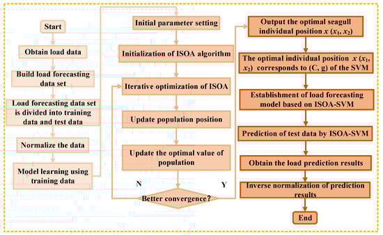
Figure 1.
Flow chart of power load forecasting based on the ISOA-SVM model.
Table 4.
Simulation pseudocode of ISOA-SVM.
4.2. Selection of Evaluation Indicators
After using the forecasting model for load forecasting, it is necessary to set evaluation indicators for the model that can evaluate the forecasting results. Therefore, four evaluation indicators are selected in this study to objectively evaluate the prediction effect of the model, including R-squared (R2), Root Mean Square Error (RMSE), Mean Absolute Error (MAE) and Mean Absolute Percentage Error (MAPE). Additionally, the evaluation indicators are shown in Equations (19)–(22).
where m is the total number of sample sets; is the real value; and is the forecasting value.
After using the prediction model to obtain the prediction results of power load, use the above four evaluation indicators, that is, comprehensively and objectively analyze the prediction effect of the model from different angles. In addition, load forecasting can be carried out by using a variety of forecasting models, and the forecasting results of the model can be used to calculate the values of the above four evaluation indicators. By comparing the differences between the prediction models, the prediction effect of the proposed ISOA-SVM model is verified.
5. Model Forecasting and Result Analysis
In this study, the data set offered by the European intelligent technology network is adopted as the experimental data, which creates statistics on the actual load data of a power plant in eastern Slovakia every 30 min [38]. In addition, literature [39] and literature [40] have also adopted this dataset and described it in more detail. To test the accuracy of the prediction model, a week of power load data, which contains 336 sample points as the data set, is selected to verify the accuracy of the model in this study.
The input of the model in this study is the load value at the same time on the day before the forecast day, the load value at the same time on the two days before the forecast day, and the load value at the same time on the same day of the previous week; The output is the load on the forecast day. Additionally, to verify the model with a different number of training set data, two cases of experiments are carried out, respectively. In Case 1, take the first five days of the week as the training data, and the 6th and 7th days as the test data; in Case 2, take the first six days of the week as the training data, and the 7th day as the test data.
In addition, to ensure the objectivity of the prediction results of each model, all models tests are operated under Windows 10 operating system and Matlab R2017a operating environment.
5.1. Case 1
In Case 1, the first five days as the power load training data, and the 6th and 7th days as the power load test data are taken as the test data. SOA-SVM, SVM and Back Propagation neural network (BP) are selected as comparison models. BP is a multilayer feedforward network trained by the error back propagation algorithm and is one of the most widely used neural network models. In this study, the parameters of BP model are set as follows: The number of input layer nodes is three; the number of hidden layer nodes is 20; the number of output layer nodes is one; the number of iterations is 100; the learning rate is 0.1; and the target value is 0.0001. And other parameters are set as default values.
The results of ISOA-SVM, SOA-SVM, SVM and BP models are shown in Figure 2. The forecasting errors of the four models are shown in Figure 3. The error histograms of four power load forecasting models for Case 1 are shown in Figure 4.
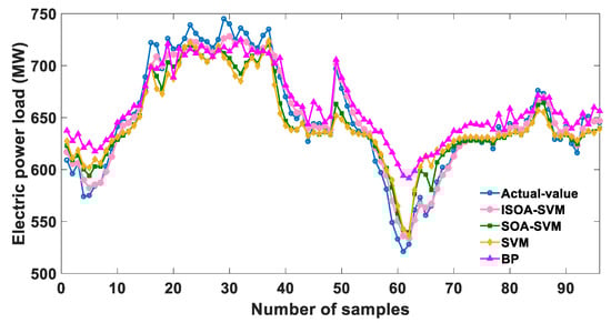
Figure 2.
Power load forecasting results of four models for Case 1.
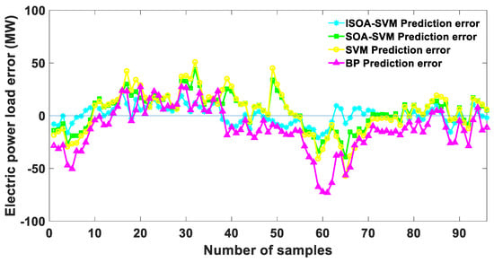
Figure 3.
Power load error of four forecasting models for Case 1.
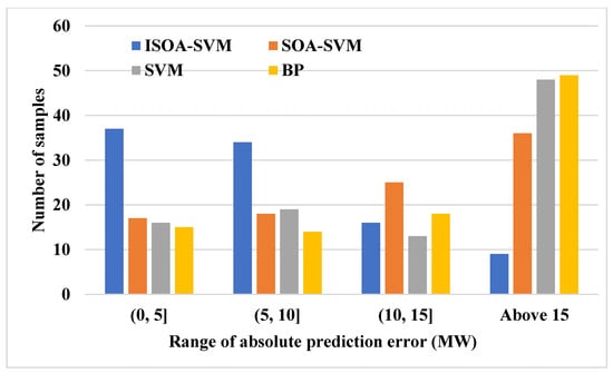
Figure 4.
The error histograms of four power load forecasting models for Case 1.
According to the forecasting results, it can be seen that the ISOA-SVM, SOA-SVM, SVM and BP model can realize the prediction of power load, but the prediction accuracy is different. As can be seen from Figure 2, the power load forecasting result of the ISOA-SVM model is closer to the real power load value than that of the SOA-SVM model. It can be seen from Figure 3 and Figure 4, compared to the SOA-SVM, that the error of the ISOA-SVM is smaller and the error sequence is smoother. It is proved that the ISOA-SVM model can better fit the power load data series, and the effectiveness of the improvement strategy of the SOA algorithm adopted in this study is verified.
To evaluate the prediction results of the model in more detail, the results of the evaluation of the power load forecasting results of Case 1 are shown in Table 5.
Table 5.
Evaluation table of power load forecasting results of Case 1.
As can be seen from Table 5, the MAE, MAPE and RMSE of SVM models are better than the BP model. In this study, the SVM model has smaller prediction error and higher prediction accuracy, which proves the accuracy of selecting the SVM model as the basic model of power load forecasting. In addition, the evaluation index results of the ISOA-SVM model are significantly better than those of the SOA-SVM model. Compared to the SOA-SVM model, the RMSE, MAPE and MAE the ISOA-SVM model decreased by 7.8783 MW, 1.0137% and 6.5844 MW, respectively. The R2 of the ISOA-SVM model is 1.611% higher than that of the SOA-SVM model. It also confirms that the proposed ISOA algorithm in this study effectively improves the optimization performance of the original algorithm. The ISOA algorithm can obtain better internal parameters of SVM through iterative optimization, so as to build a model to achieve high-precision power load forecasting.
5.2. Case 2
In Case 2, the first six days as the power load training data, and the 7th days as the power load test data are taken as the test data. SOA-SVM, SVM and BP are also selected as comparison models. The prediction results of ISOA-SVM, SOA-SVM, SVM and BP models of Case 2 are shown in Figure 5. The forecasting errors of the four models of Case 2 are shown in Figure 6. The error histograms of four power load forecasting models for Case 2 are shown in Figure 7.
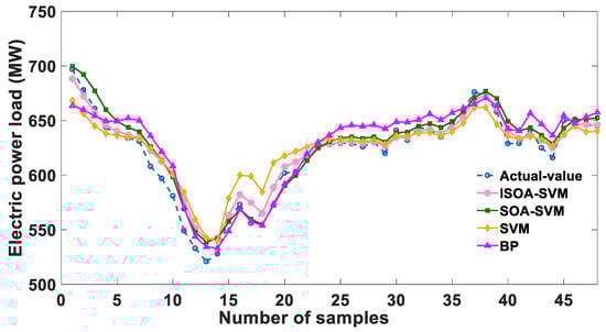
Figure 5.
Power load forecasting results of four models for Case 2.
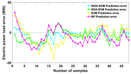
Figure 6.
Power load error of four forecasting models for Case 2.
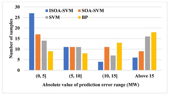
Figure 7.
The error histograms of four power load forecasting models for Case 2.
It can be shown, in Table 6, the prediction results of the each power load model in Case 2 by using the evaluation indicators.
Table 6.
Evaluation table of the power load forecasting results of Case 2.
As can be seen from Figure 4 and Figure 5 that the prediction accuracy of the ISOA-SVM model is better than that of the SOA-SVM, SVM and BP models. It can be seen from Table 6 that the MAE, MAPE and RMSE of the ISOA-SVM model are lower, which are 6.6434 MW, 1.1179% and 9.2442 MW, respectively. Compared to the SOA-SVM model, MAE, MAPE and RMSE of the ISOA-SVM model decreased by 2.1533 MW, 0.3303% and 1.2468 MW, respectively. Compared with SVM model, the RMSE, MAPE and MAE of SOA-SVM decreased by 4.624 MW, 0.5119% and 2.9763 MW, respectively. From the above analysis, it can be found that the power load result of using ISOA algorithm to optimize SVM model is better than SOA-SVM and traditional single SVM model. Thus, the effectiveness of the proposed ISOA-SVM power load forecasting model is proved.
This study carried out a prediction study on this group of load data, showing a stronger prediction accuracy and stability. More experiments will be done in the future to further demonstrate the universality and superiority of the proposed method.
6. Conclusions
High precision power load forecasting can provide decision makers with scientific power generation plans, and reasonably arrange the plan for the start-up and shut-down of units to ensure the stability and safety of the power system operating. In addition, high accuracy electric load forecasting can effectively reduce power generation costs, improve energy utilization, improve social benefit and economic benefit. This study contributes to enhance the predicted accuracy of electric load. In this study, in view of the slow convergence speed of the SOA, three strategies are proposed to improve optimization performance and convergence accuracy of SOA, and an ISOA algorithm with better optimization performance and higher convergence accuracy is proposed. Additionally, the ISOA algorithm is used to optimize the internal parameters of SVM, a high-precision power load forecasting model based on the ISOA-SVM is built. Further, the effectiveness and accuracy of the model proposed in this study are verified by two cases. Additionally, this study can provide scientific instruction for the power generation and power consumption planning.
While the model proposed in this study has achieved satisfactory prediction results, this study also has some limitations: (1) The generalization ability and prediction stability of the proposed prediction model need to be further improved; and (2) the universality of the prediction ability of the model needs to be further strengthened. In the follow-up study, we will focus on solving these limitations.
Author Contributions
S.Z.: Conceptualization, Methodology, Original writing. N.Z.: Conceptualization, Methodology, Original writing. Z.Z.: Methodology, Original writing. Y.C.: Methodology, Original writing. All authors have read and agreed to the published version of the manuscript.
Funding
This research received no external funding.
Data Availability Statement
The raw data supporting this paper is available and will be provided without reservation by contacting the corresponding author if necessary.
Conflicts of Interest
The authors declare that the research was conducted in the absence of any commercial or financial relationships that could be construed as a potential conflict of interest.
References
- Aslam, S.; Herodotou, H.; Mohsin, S.M.; Javaid, N.; Ashraf, N.; Aslam, S. A survey on deep learning methods for power load and renewable energy forecasting in smart microgrids. Renew. Sustain. Energy Rev. 2021, 144, 110992. [Google Scholar] [CrossRef]
- Liu, K.; Ashwin, T.R.; Hu, X.; Lucu, M.; Widanage, W.D. An evaluation study of different modelling techniques for calendar ageing prediction of lithium-ion batteries. Renew. Sustain. Energy Rev. 2020, 131, 110017. [Google Scholar] [CrossRef]
- Li, J.; Chen, L.; Xiang, Y.; Li, J.; Peng, D. Influencing Factors and Development Trend Analysis of China Electric Grid Investment Demand Based on a Panel Co-Integration Model. Sustainability 2018, 10, 256. [Google Scholar] [CrossRef]
- Al-Dahidi, S.; Baraldi, P.; Zio, E.; Montelatici, L. Bootstrapped Ensemble of Artificial Neural Networks Technique for Quantifying Uncertainty in Prediction of Wind Energy Production. Sustainability 2021, 13, 6417. [Google Scholar] [CrossRef]
- Raza, M.Q.; Khosravi, A. A review on artificial intelligence based load demand forecasting techniques for smart grid and buildings. Renew. Sustain. Energy Rev. 2015, 50, 1352–1372. [Google Scholar] [CrossRef]
- Butt, F.M.; Hussain, L.; Jafri, S.H.M.; Alshahrani, H.M.; Al-Wesabi, F.N.; Lone, K.J.; El Din, E.M.T.; Al Duhayyim, M. Intelligence based Accurate Medium and Long Term Load Forecasting System. Appl. Artif. Intell. 2022, 36, 2088452. [Google Scholar] [CrossRef]
- Akhter, M.N.; Mekhilef, S.; Mokhlis, H.; Shah, N.M. Review on forecasting of photovoltaic power generation based on machine learning and metaheuristic techniques. IET Renew. Power Gener. 2019, 13, 1009–1023. [Google Scholar] [CrossRef]
- Li, L.-L.; Zhao, X.; Tseng, M.-L.; Tan, R.R. Short-term wind power forecasting based on support vector machine with improved dragonfly algorithm. J. Clean. Prod. 2020, 242, 118447. [Google Scholar] [CrossRef]
- Lai, C.S.; Locatelli, G.; Pimm, A.; Wu, X.; Lai, L.L. A review on long-term electrical power system modeling with energy storage. J. Clean. Prod. 2021, 280, 124298. [Google Scholar] [CrossRef]
- Ahmad, T.; Zhang, H.; Yan, B. A review on renewable energy and electricity requirement forecasting models for smart grid and buildings. Sustain. Cities Soc. 2020, 55, 102052. [Google Scholar] [CrossRef]
- Niu, D.X.; Yu, M.; Sun, L.J.; Gao, T.; Wang, K.K. Short-term multi-energy load forecasting for integrated energy systems based on CNN-BiGRU optimized by attention mechanism. Appl. Energy 2022, 313, 118801. [Google Scholar] [CrossRef]
- Agüero, J.; Rodríguez, F.; Giménez, A. Energy management based on productiveness concept. Renew. Sustain. Energy Rev. 2013, 22, 92–100. [Google Scholar] [CrossRef]
- Zhu, R.; Guo, W.; Gong, X. Short-Term Load Forecasting for CCHP Systems Considering the Correlation between Heating, Gas and Electrical Loads Based on Deep Learning. Energies 2019, 12, 3308. [Google Scholar] [CrossRef]
- Han, L.; Peng, Y.; Li, Y.; Yong, B.; Zhou, Q.; Shu, L. Enhanced Deep Networks for Short-Term and Medium-Term Load Forecasting. IEEE Access 2018, 7, 4045–4055. [Google Scholar] [CrossRef]
- Haben, S.; Arora, S.; Giasemidis, G.; Voss, M.; Greetham, D.V. Review of low voltage load forecasting: Methods, applications, and recommendations. Appl. Energy 2021, 304, 117798. [Google Scholar] [CrossRef]
- Chitalia, G.; Pipattanasomporn, M.; Garg, V.; Rahman, S. Robust short-term electrical load forecasting framework for commercial buildings using deep recurrent neural networks. Appl. Energy 2020, 278, 115410. [Google Scholar] [CrossRef]
- Dunea, D.; Iordache, S. Time Series Analysis of the Heavy Metals Loaded Wastewaters Resulted from Chromium Electroplating Process. Environ. Eng. Manag. J. 2011, 10, 421–434. [Google Scholar] [CrossRef]
- Farahat, M.A.; Talaat, M. Short-Term Load Forecasting Using Curve Fitting Prediction Optimized by Genetic Algorithms. Int. J. Energy Eng. 2012, 2, 23–28. [Google Scholar] [CrossRef]
- Dudek, G. Artificial Immune Clustering Algorithm to Forecasting Seasonal Time Series. Lect. Notes Comput. Sci. 2011, 6922, 468–477. [Google Scholar] [CrossRef]
- García-Ascanio, C.; Maté, C. Electric power demand forecasting using interval time series: A comparison between VAR and iMLP. Energy Policy 2010, 38, 715–725. [Google Scholar] [CrossRef]
- Khatoon, S.; Singh, A.K. ANN based Electric Load Forecasting Applied to Real Time Data. In Proceedings of the Annual IEEE India Conference (INDICON), New Delhi, India, 17–20 December 2015. [Google Scholar]
- Xu, X.; Niu, D.; Fu, M.; Xia, H.; Wu, H. A Multi Time Scale Wind Power Forecasting Model of a Chaotic Echo State Network Based on a Hybrid Algorithm of Particle Swarm Optimization and Tabu Search. Energies 2015, 8, 12388–12408. [Google Scholar] [CrossRef]
- Aneiros, G.; Vilar, J.; Raña, P. Short-term forecast of daily curves of electricity demand and price. Int. J. Electr. Power Energy Syst. 2016, 80, 96–108. [Google Scholar] [CrossRef]
- Cho, H.; Goude, Y.; Brossat, X.; Yao, Q. Modeling and Forecasting Daily Electricity Load Curves: A Hybrid Approach. J. Am. Stat. Assoc. 2013, 108, 7–21. [Google Scholar] [CrossRef]
- Wang, S.; Wang, X.; Wang, S.; Wang, D. Bi-directional long short-term memory method based on attention mechanism and rolling update for short-term load forecasting. Int. J. Electr. Power Energy Syst. 2019, 109, 470–479. [Google Scholar] [CrossRef]
- Bo, H.; Nie, Y.; Wang, J. Electric Load Forecasting Use a Novelty Hybrid Model on the Basic of Data Preprocessing Technique and Multi-Objective Optimization Algorithm. IEEE Access 2020, 8, 13858–13874. [Google Scholar] [CrossRef]
- Li, C. A fuzzy theory-based machine learning method for workdays and weekends short-term load forecasting. Energy Build. 2021, 245, 111072. [Google Scholar] [CrossRef]
- Ge, Q.; Jiang, H.; He, M.; Zhu, Y.; Zhang, J. Power Load Forecast Based on Fuzzy BP Neural Networks with Dynamical Estimation of Weights. Int. J. Fuzzy Syst. 2020, 22, 956–969. [Google Scholar] [CrossRef]
- Yuan, C.H.; Niu, D.X.; Li, C.Z.; Sun, L.J.; Xu, L.X. Electricity Consumption Prediction Model Based on Bayesian Regularized BP Neural Network. Cyber Secur. Intell. Anal. 2020, 928, 528–535. [Google Scholar]
- Wang, Z.; Wang, X.; Ma, C.; Song, Z. A Power Load Forecasting Model Based on FA-CSSA-ELM. Math. Probl. Eng. 2021, 2021, 9965932. [Google Scholar] [CrossRef]
- Li, W.; Quan, C.; Wang, X.; Zhang, S. Short-Term Power Load Forecasting Based on a Combination of VMD and ELM. Pol. J. Environ. Stud. 2018, 27, 2143–2154. [Google Scholar] [CrossRef]
- Zhang, A.A.; Zhang, P.X.; Feng, Y.T. Short-term load forecasting for microgrids based on DA-SVM. COMPEL Int. J. Comput. Math. Electr. Electron. Eng. 2019, 38, 68–80. [Google Scholar] [CrossRef]
- Dong, X.; Deng, S.; Wang, D. A short-term power load forecasting method based on k-means and SVM. J. Ambient Intell. Humaniz. Comput. 2021, 13, 5253–5267. [Google Scholar] [CrossRef]
- Yang, A.; Li, W.; Yang, X. Short-term electricity load forecasting based on feature selection and Least Squares Support Vector Machines. Knowledge-Based Syst. 2019, 163, 159–173. [Google Scholar] [CrossRef]
- Ma, W.; Zhang, X.; Xin, Y.; Li, S. Study on short-term network forecasting based on SVM-MFA algorithm. J. Vis. Commun. Image Represent. 2019, 65, 102646. [Google Scholar] [CrossRef]
- Hsndl, J.; Knowles, J. An evolutionary approach to multi-objective clustering. IEEE Trans. Evol. Comput. 2006, 11, 56–76. [Google Scholar]
- Yue, C.T.; Qu, B.Y.; Yu, K.J.; Liang, J.; Li, X.D. A novel scalable test problem suite for multimodal multi objective optimization. Swarm Evol. Comput. 2019, 48, 62–71. [Google Scholar] [CrossRef]
- Available online: https://www.iteye.com/resource/huan_chen-10191360 (accessed on 20 March 2021).
- Chen, B.J.; Chang, M.W.; Lin, C.J. Load Forecasting Using Support Vector Machines: A Study on EUNITE Competition 2001. IEEE Trans. Power Syst. 2004, 19, 1821–1830. [Google Scholar] [CrossRef]
- Tang, X.L.; Dai, Y.Y.; Wang, T.; Chen, Y.J. Short-term power load forecasting based on multi-layer bidirectional recurrent neural network. IET Gener. Transm. Distrib. 2019, 13, 3847–3854. [Google Scholar] [CrossRef]
Publisher’s Note: MDPI stays neutral with regard to jurisdictional claims in published maps and institutional affiliations. |
© 2022 by the authors. Licensee MDPI, Basel, Switzerland. This article is an open access article distributed under the terms and conditions of the Creative Commons Attribution (CC BY) license (https://creativecommons.org/licenses/by/4.0/).