Article

Thermal Modeling and Prediction of The Lithium-ion Battery Based on Driving Behavior

School of Mechanical and Power Engineering, Zhengzhou University, Zhengzhou 450001, China
*
Author to whom correspondence should be addressed.
Energies 2022, 15(23), 9088; https://doi.org/10.3390/en15239088
Submission received: 25 October 2022 / Revised: 17 November 2022 / Accepted: 28 November 2022 / Published: 30 November 2022
(This article belongs to the Section E: Electric Vehicles)

Abstract

:
Real-time monitoring of the battery thermal status is important to ensure the effectiveness of battery thermal management system (BTMS), which can effectively avoid thermal runaway. In the study of BTMS, driver behavior is one of the factors affecting the performance of the battery thermal status, and it is often neglected in battery temperature studies. Therefore, it is necessary to predict the dynamic heat generation of the battery in actual driving cycles. In this work, a thermal equivalent circuit model (TECM) and an artificial neural network (ANN) thermal model based on the driving data, which can predict the thermal behavior of the battery in real-world driving cycles, are proposed and established by MATLAB/Simulink tool. Driving behaviors analysis of different drivers are simulated by PI control as input, and battery temperature is used as output response. The results show that aggressive driving behavior leads to an increase in battery temperature of nearly 1.2 K per second, and the average prediction error of TECM model and ANN model is 0.13 K and 0.11 K, respectively. This indicates that both models can accurately estimate the real-time battery temperature. However, the computational speed of the ANN thermal model is only 0.2 s, which is more efficient for battery thermal management.

1. Introduction

The development of the automotive sector is motivated by international environmental protection policies, focusing on low-carbon transportation. Recent years have seen an increase in the conversion of urban public transportation vehicles and private cars from fuel vehicles to electric vehicles (EVs) due to purchase subsidies for new energy vehicles and the widespread use of public charging stations [1,2]. The substantial market demand for pure electric vehicles encourages the quick advancement of battery technology. Moreover, lithium-ion battery (LIB) has high specific power and energy density, which has great potential to replace the internal combustion engine as the main power source of automobiles [3,4,5]. However, the heat generated by the operation of LIB might significantly compromise the safety of EVs [6,7,8,9]. Continuous discharge causes the internal temperature of the battery to grow, which drastically reduces battery performance because the internal heat of the LIB pack cannot be dispersed over time. At the same time, constantly operating at high temperatures would cause thermal runaway in addition to accelerating battery degradation [10,11]. It has been found that ensuring that the LIB pack operates within the optimal temperature range of 15 °C to 35 °C and the temperature difference of the LIB pack is less than 5 °C will significantly lengthen the battery life [12], [13]. Therefore, in order to ensure that the battery functions in the optimal temperature range and avoid thermal runaway caused by excessive temperatures, it is necessary to establish an accurate prediction model of battery heat for monitoring the battery thermal state.
The most commonly used battery thermal models are the electrochemical–thermal coupling model, the thermal equivalent circuit model (TECM), and the data-based model [14]. Xu et al. [15] investigated the thermal runaway phenomenon of LIBs at high temperatures by developing an electrochemical–thermal coupling model that was used to analyze the heat generated by five different types of battery side reactions. However, in practice, the complexity of electrochemical reactions and the numerous sets of partial differential equations that must be calculated in the model lead to slow calculations that do not meet the needs of thermal management systems for real-time temperature estimation [16,
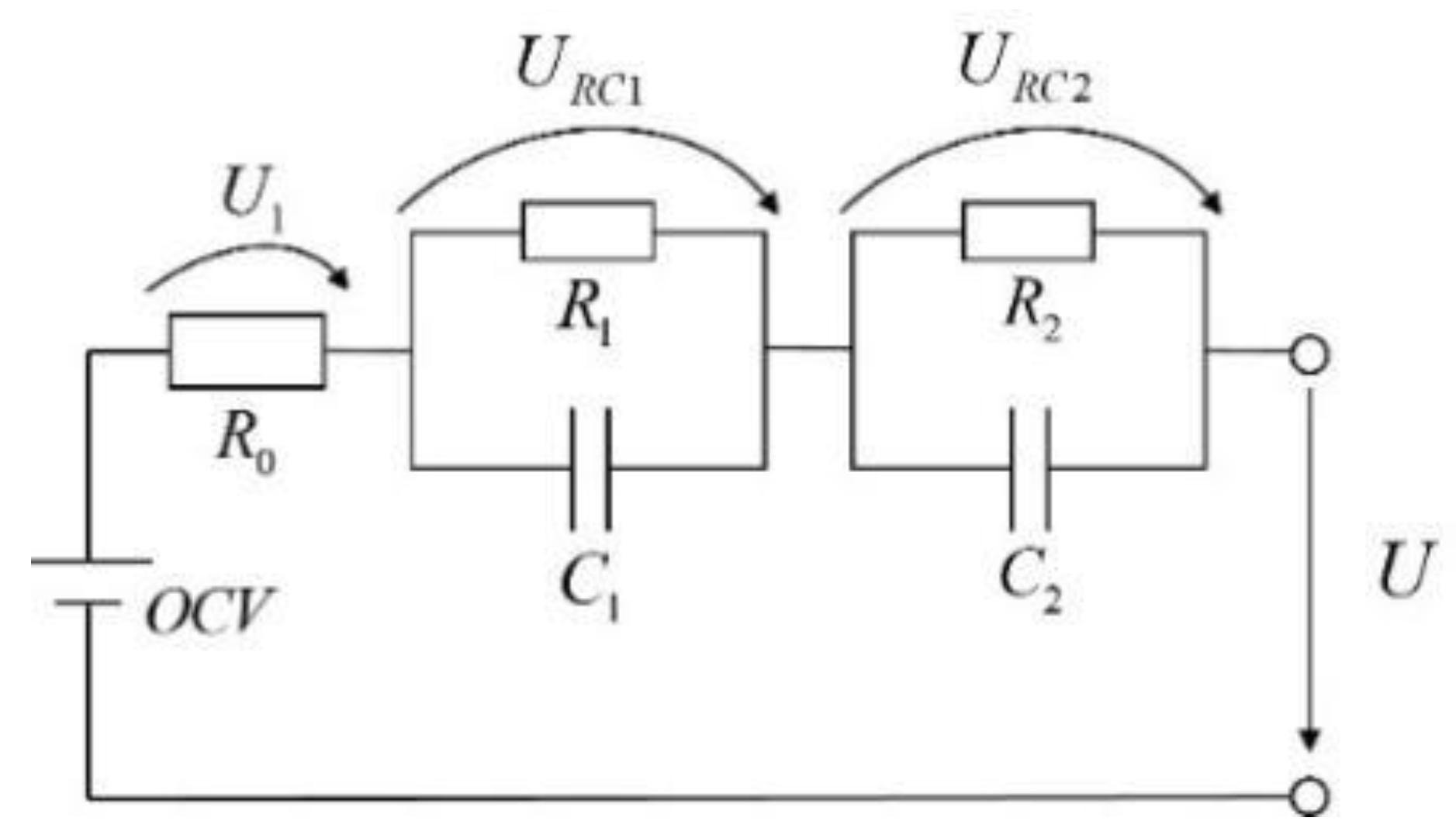
17]. TECM is more concise in modeling and better suited for simulating the dynamic behavior of the battery than the electrochemical–thermal coupling model. It was discovered in [18] that one or two RC networks in the equivalent circuit were sufficient to satisfy the electrical behavior. It was unnecessary to use higher-order RC networks for greater accuracy, which would increase the model’s complexity and computation time. Nejad et al. [19] compared equivalent circuit models of two cell types, LiFePO4 and LiNMC, for different orders and found that the model with two RC circuits is preferable for describing the dynamic properties of the cell [20,21]. However, the temperature estimation model was not used in those studies. Geifes et al. [22] developed a first-order thermal equivalent circuit model for small cells and experimentally tested its accuracy. Only estimating the temperature of the battery is insufficient in a practical BTMS application. For BTMS, a real-time model with a prediction function is required, which has contributed to the growth of data-driven battery thermal models. The data-driven model does not need to consider the battery’s physical parameters, but rather establishes a link between the input parameters and the battery’s output response using machine learning methods such as support vector machines [23] or neural networks [24]. The neural network model is more advantageous in establishing nonlinear dynamic relationships. Zhuang et al. [25] proposed a battery prediction model by combining a lithium-ion equivalent circuit model with a fuzzy model. The battery temperature prediction model was able to obtain pack temperature information in advance to achieve active cooling of the battery. Kleiner et al. [26] developed a 3D electro-thermal prediction model for prismatic cells and validated the model temperature prediction with laboratory scenarios. Xie et al. [27] combined the dynamic resistance model with the current distribution model to propose a new electro-thermal model, and verified the accuracy of temperature prediction under the conditions of static and dynamic currents. However, general thermal models often use a feed-forward neural network (FFNN), which can only estimate the cell temperature and cannot feed the estimates back to the input for achieving multi-step heat prediction. In contrast, the NARX neural network is sufficient to achieve feed-forward estimation and feed-back prediction, and has a good advantage in solving the prediction problem of time series. Most of the literature on battery thermal modeling has only used simple constant current charge/discharge or standard driving cycle conditions to test the model’s accuracy, without fully considering the driver data in a real driving cycle as the input variables affecting the battery temperature for the study. Jafari et al. [
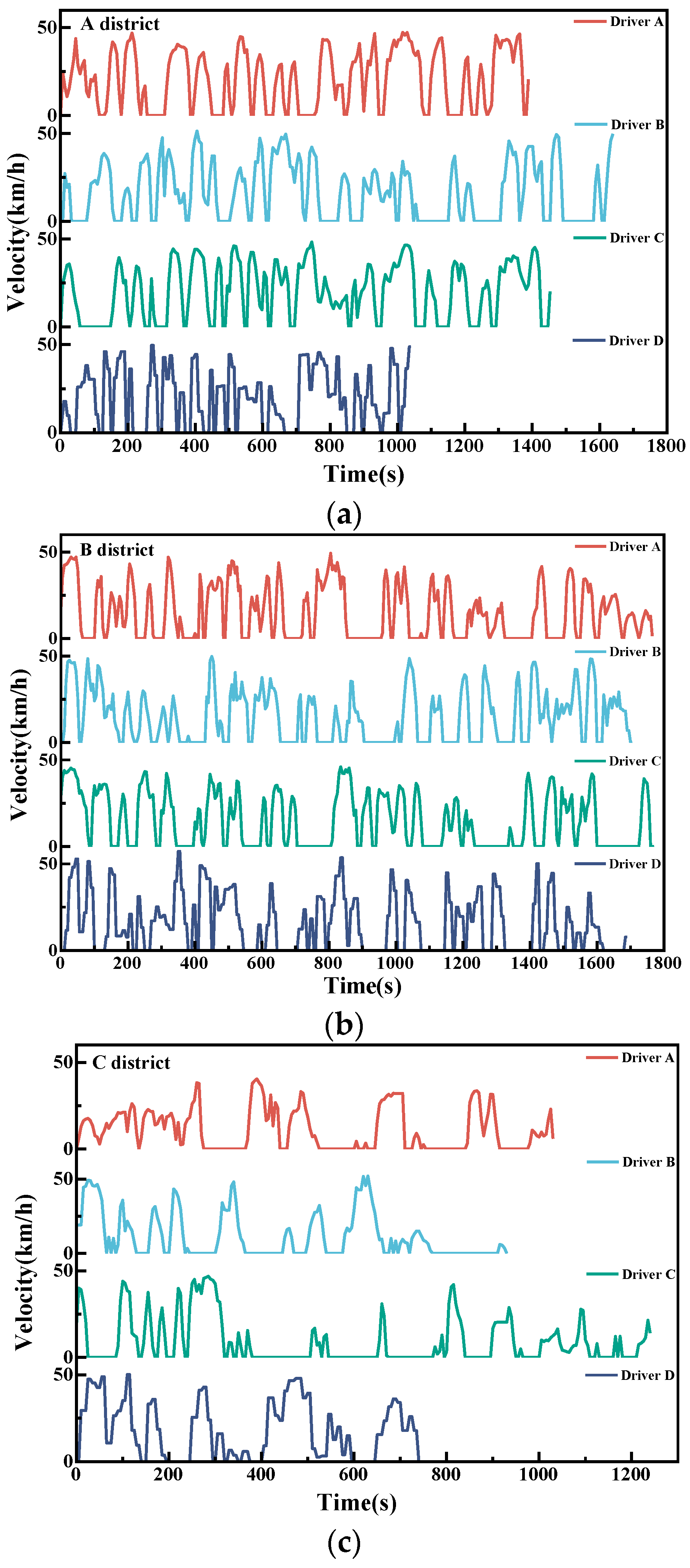
28] investigated the effect of driving style on battery capacity decay by using real-driving cycle data. Mudgal et al. [29] found that aggressive driving behavior increases energy consumption by 5–33%. The increased energy consumption is used to cool the temperature rise caused by aggressive driving [30]. Aggressive driving behavior increases the instantaneous current and leads to a rapid increase in battery temperature [31], while gentle driving behavior enables a smooth discharge of the LIB and the internal temperature of the battery does not rapidly rise. However, there is little literature focused on the influence of driving behavior on the internal temperature of battery. As a consequence, research into the effect of driving behavior on battery heating is important.
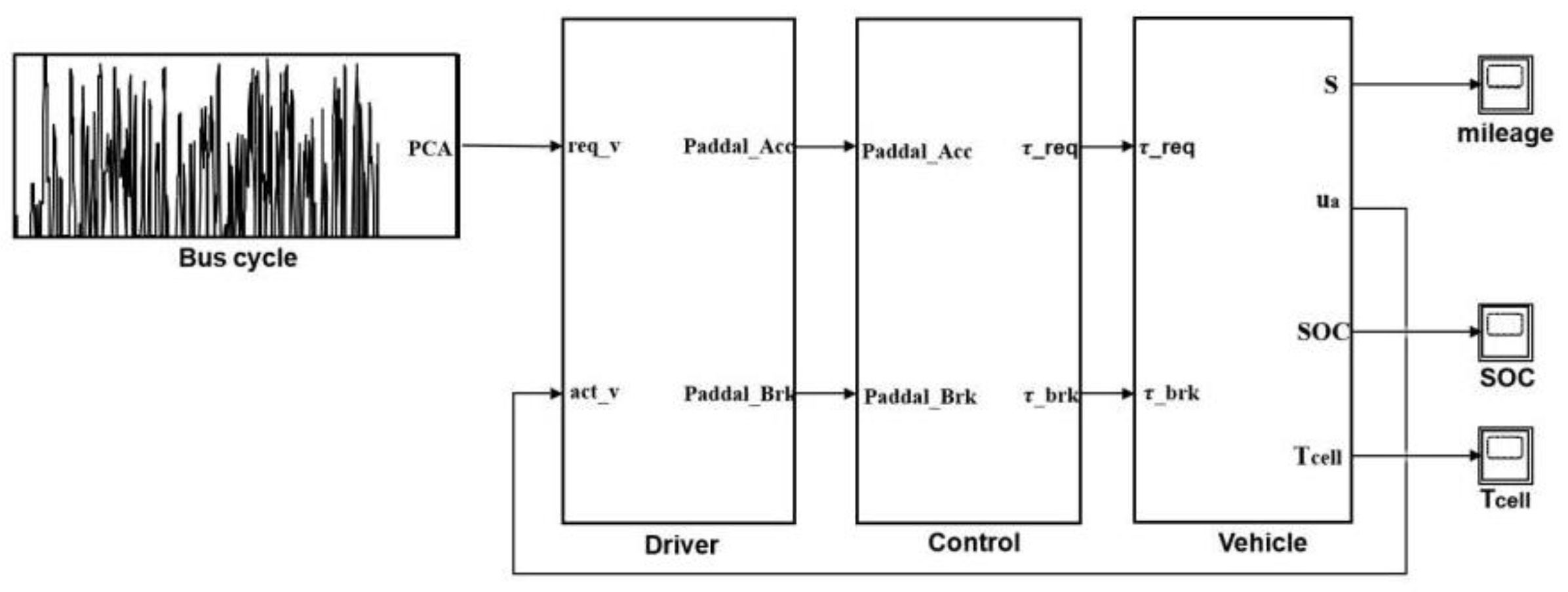
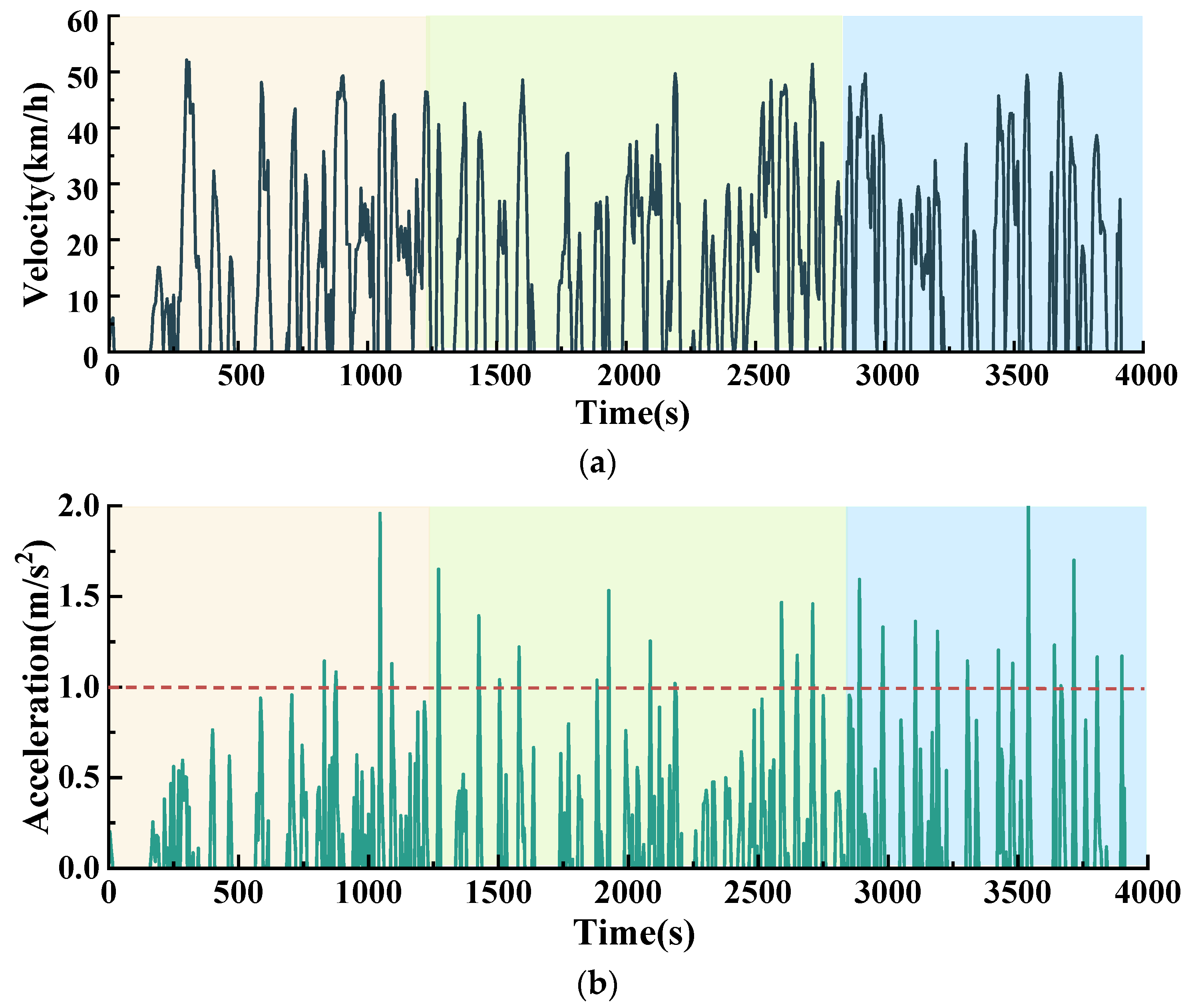
To fill this void, the influence of driving behavior parameters on battery temperature is investigated in this study. Based on actual driving cycles, TECM and ANN thermal models with driver behavior parameters as input are proposed and built in MATLAB/Simulink software. In terms of driving behavior, ambient temperature, state of charge (SOC), discharge rate, and other factors, the effects of battery temperature and internal physical parameters on battery performance are examined. The two proposed models’ temperature prediction results are compared in terms of calculation speed and accuracy.
The remaining sections of this article are structured as follows: In Section 2, a TECM based on a LiFePO4 cell with a total capacity of 20 Ah is established; In Section 3, the PCA method is used to obtain the primary parameters describing the driver behavior by reducing the data dimension of the collected driver behavior data; The EV model is established and the temperature prediction of TECM and ANN models influenced by driving behavior is analyzed in Section 4; Section 5 is the summary and prospect of this article.

2. Thermal Equivalent Circuit Model

The battery model is the core part of this study, as it is the only source of power in the vehicle and its performance has a direct impact on real driving. Firstly, the equivalent circuit model based on the LiFePO4 cell is introduced, and then the nonlinear relationship between the physical parameters, SOC, and temperature of the cell is described. The heat generation model is based on the description of the heat generation equation established by Bernardi et al. [32]. Finally, the equivalent circuit model is coupled with the thermal model to establish a TECM.

2.1. Equivalent Circuit Model

(a) Single-cell electrical model: A square LiFePO4 cell with a nominal voltage of 3.2 V and a total capacity of 20 Ah is used as a single cell for experimental verification. The equivalent circuit model is shown in Figure 1, which consists of a voltage source, an ohmic resistance R0 and two parallel RCs, and the polarization resistances R1, R2 can respond to the voltage drop caused by overvoltage [33]. The battery terminal voltage can be expressed as follows:
U = O C V I R 0 U R C 1 U R C 2 ,
d U R C 1 d t + U R C 1 R 1 C 1 = I C 1 ,
d U R C 2 d t + U R C 2 R 2 C 2 = I C 2 ,
where U is the terminal voltage and I is the battery current. OCV is open circuit voltage; URC1 and URC2 are the polarization voltages of the battery. R0, R1, R2, C1 and C2 are functions of current, temperature, and SOC as defined by Equation (4).
R 0 , R 1 , R 2 , C 1 , C 2 = f ( I , T , S O C ) .
The resistance, capacitance, and open circuit voltage (OCV) in the equivalent circuit are affected by the ambient temperature, the internal temperature, and the SOC. The cell parameters were determined by hybrid pulse power characteristic (HPPC) [34], which are shown in Table 1. The HPPC test was performed for ambient temperature from 15 °C to 45 °C, the SOC from 0.1 to 1 at a 0.1 interval each time and the current range from 0.5 C to 3 C (1 C = 20 A) to identify the battery parameters. The battery test equipment includes a main controller, a thermostat, and a data acquisition unit, which is shown in Figure 2. The voltage and current curves at an ambient temperature of 25 °C are demonstrated in Figure 3. The voltage–current curves from the experimental data were fitted to the polarization resistances R1 and R2 by the MATLAB fitting toolbox. The relationship between the impedance parameters and the current, the SOC, and the temperature are shown in Figure 4, Figure 5 and Figure 6.
At the same discharge rate, the Ohmic resistance and polarization resistance increase with decreasing temperature and SOC; they decrease with increasing discharge rate when the temperature is constant. The experimental results correspond with the Butler–Volmer equation (BV) (the resistance decreases with increasing discharge current due to the influence of charge transfer within the cell. When the current is tiny, the ability of lithium-ions to cross the interfacial barrier is weak, and the polarization resistance rises sharply). In addition, all test data regression values for impedance parameter identification are higher than 0.9995.
(b) Battery pack electrical model: The battery pack is arranged in the form of 20P160S. In this work, it is assumed that the electrical and thermal parameters of the single cell in the battery pack are the same. Therefore, the battery pack voltage Upac and capacity Cpac are as follows:
U p a c = 160 U ,
C p a c = 20 C .

2.2. Battery Thermal Model

Battery heat generation is calculated by Bernardi’s formula:
Q = ( O C V U ) I + T c e l l I d O C V d T ,
Q = I 2 R 0 + I 2 R 1 + I 2 R 2 + I T c e l l d O C V d T ,
where I2R0 + I2R1 + I2R2 is the irreversible heat generated by the voltage drop due to the resistance in the Joule reaction, which always has a positive value; ITcell (dOCV/dT) is the reversible heat of reaction resulting from an entropic change caused by an electrochemical reaction, the positivity or negativity of which is influenced by the direction of the current. dOCV/dT is the entropy coefficient. The relationship between OCV, SOC and temperature is shown in Figure 7.
To simplify the calculations, the thermal behavior of the cell thickness direction is neglected [35], and it is assumed that the heat generation is uniform and consistent in the battery pack. Therefore, the heat generation of the battery pack Qpac is as follows:
Q p a c = 160 Q .
According to Newton’s law of cooling, the heat to be dissipated by the battery pack is
Q c o n v = h A ( T c e l l T ) ,
where h is the heat exchange coefficient between the battery pack and the coolant, A is the heat dissipation area of the battery pack, Tcell is the actual battery temperature, and T is the ambient temperature. The heat exchange coefficient h needs to be identified by the thermal characteristic test. The model established in this paper is only used for temperature identification, while the thermostat is used to insulate the test battery, so Qconv is set to zero.
When thermal management of the battery pack is performed, the internal heat of the battery can be expressed as
Q p a c Q c o n v = m b a t C b a t d T d t ,
where mbat is the concentrated mass of the cell, cbat is the heat capacity of the cell.

2.3. Model Validation and Analysis

A common validation for the battery model is to conduct the charge–discharge test under constant current, while in real-world driving cycles the current is real-time. Therefore, the standard driving cycle, NEDC, is used to verify the accuracy of the battery model. The accuracy of the simulation results and experimental data is evaluated by the root mean square error (RMSE) and mean absolute error (MAE).
MAE = 1 t i = 1 t | y t u t | ,
RMSE = 1 k t = 1 k ( y t u t ) 2 ,
where yt is the simulated value, ut is the experimental value, k is the number of sampling points, and t is the experiment time.
The accuracy of the model at dynamic current are verified with NEDC cycle at ambient temperature settings of 15–45 °C (10 °C interval). This result is presented in Figure 8, where the simulated and experimental battery voltages are depicted, and the voltage error of the model is less than 0.03 V.
The thermocouple is uniformly arranged at five sampling points of the battery during temperature collection. Because the temperature difference between the five sampling points is small, the single cell is regarded as a uniform heating body in the data processing stage, and the measured temperature is averaged. The estimated temperature data and experimental data are shown in Figure 9. The MAE and RMES values of the battery voltage at different ambient temperatures under NEDC cycle are depicted in Table 2, and they visually illustrate that the model performs better with dynamic input response. The TECM built in this paper satisfies the accuracy at dynamic current to simulate the battery charging and discharging. However, the acceleration of NEDC conditions is minimal, which is gentle driving behavior. In actual driving, aggressive driving accounts for a large proportion. To design a more accurate battery model, the actual driver behavior should be analyzed for real driving cycles.

3. Driver Behavior

3.1. Driver Behavior Data Collection

Driving data are collected through a communication system in the vehicle such as Controller Area Network (CAN) which enables information exchange between electronic control units (ECU) and sensors. The data in this article are obtained from one month of driving data on the same bus route. Driving data include the total travel time, SOC, route length, speed, acceleration, accelerator pedal opening (AP), maximum acceleration, maximum deceleration, average speed driving, etc. The bus passes through three areas and the route are shown in Figure 10. A district is a typical suburban area with wide roads and light traffic. B district is an urban area with more traffic lights and traffic flow, and it takes more time for bus to pass through this area than A district at the same distance. C district is the city center with narrow roads and contains densely populated areas such as shopping malls and train stations. Part of the drivers driving speed data on the bus route in A, B, C districts is shown in Figure 11.
Based on the information of acceleration, the driving styles are classified as Aggressive and Gentle. Rapid acceleration and deceleration indicate aggressive driving behavior; smooth acceleration and deceleration represent gentle behavior in driving cycle. Analysis of the data reveal that aggressive driving behavior occurs when buses are entering and exiting stations, overtaking and changing lanes. While gentle driving with smooth acceleration, the buses often run at a constant speed or at low speeds close to idle on crowded roads. Classification of vehicle driving styles is usually based on driver and occupant comfort, and an acceleration of 2 m/s2 is used as a boundary to determine whether a driver is driving aggressively. However, for buses with high center of gravity and high carriage, a very small acceleration in their driving can cause large roll angle. Therefore, it is scientific to classify bus driving styles with acceleration values smaller than those of the car. Classification of bus driving styles by acceleration values is shown in Table 3.
Correlations may exist between driving parameters, and using all of these data for calculation tends to increase the computing time. Therefore, the collected parameters should be pre-processed before constructing the driver model.

3.2. Driver Behavior Data Analysis

The principal component analysis (PCA) method orthogonally transforms multiple correlated variables into a new set of fewer variables in order to reduce data dimensionality and facilitate data analysis [36]. The PCA algorithm is used to orthogonally transform the interrelated driving behavior parameter samples into a linearly uncorrelated feature matrix, and the principal component contribution is analyzed to filter the representative principal components to reflect the driving behavior characteristics. This algorithm can be used to reduce the dimensionality of driving behavior parameters.
Table 4, Table 5, Table 6, Table 7 and Table 8 show the extracted driving behavior parameters for various drivers. Because the units between these variables differ, normalizing the variables at different scales is required before using the PCA method for dimensionality reduction.
The effects of average speed, maximum speed, average acceleration, maximum acceleration, average deceleration, maximum deceleration, and idle ratio on battery temperature during driving cycles are analyzed. Different variables are used to verify the validity of the PCA: Kaiser–Meyer–Olkin (KMO) test, Bartlett’s test, eigenvalue, and cumulative contribution rate. Firstly, the KMO value should be greater than 0.6, and the significance should be less than 0.05. Secondly, eigenvalues are used to measure standardized data, and its value greater than 1 indicates that the component is significant. Finally, the cumulative percentage should be around 85%. As shown in Table 8, the KMO value is 0.755 and the Bartlett significance value is 0, indicating that the factor analysis is valid. In Table 9, it is shown that the eigenvalue of PC1 is 3.565, accounting for 50.925% of the total components; the eigenvalue of PC2 is 1.626, accounting for 23.232% of the total components; and the eigenvalue of PC3 is 1.064, accounting for 15.205% of the total components. Using these three principal components, 89.362% of the variance in the complete data can be represented.
According to the component scores shown in Table 10, the average acceleration and maximum acceleration are the main components of PC1; the average speed is the main component of PC2, and the idling ratio is the main component of PC3. Therefore, the seven variables indicating driving behaviors are transformed into three principal components by the PCA algorithm to provide data for building the driver model.

3.3. Driver Model

Through driving behavior analysis, the average speed, average acceleration, maximum acceleration and idle ratio are determined as inputs to the driver model. The sampling time of the thermal model is 1 s. To compensate for the 1 s time lag, a speed prediction PI controller is established in the driver model to ensure the synchronization between the input speed value u1 and the output temperature value T1 in the driver model at the moment t1. The desired AP within the bus driving cycle is controlled by simulating the real driver behavior. The PI control is as follows:
u ( t ) = k p e ( t ) + k i 0 t e ( t ) d t ,
where u(t) is bus torque compensation value adjusted by PI controller, it is the control variable; e(t) is the deviation between the desired speed and the predicted speed; kp is the proportional coefficient, the larger the value the faster the system response; ki is the integral coefficient, the smaller the value the faster the elimination of system static error. Therefore, the required torque Tprop of the bus and AP are as follows:
T p r o p = m a x { 0 , u ( t ) + T t q } ,
A P = T p r o p T m a x · u a · 100 % ,
where τ t q is motor torque; τ m a x is the maximum torque of the motor. Based on the driving data analysis and the above battery thermal model, the EV model is built in MATLAB/Simulink by coupling each subsystem, which consists of driver, control and electrical system, as shown in Figure 12.
The driver model outputs the accelerator pedal signal, which is used by the control system as input to simulate the motor load, and the required torque is fed back to the electrical system to control the motor drive. The electrical system includes the battery model, the motor model, and the dynamic model. Torque and wheel speed are converted into required power and current through the motor model to the dynamic model. The driving cycle without climbing condition is studied in this article. Therefore, the bus tractions Ftrac are considered as the sum of the rolling resistance Ff, the air resistance Fw, and the acceleration resistance Fj.
F t r a c = F f + F w + F j ,
τ r = m g f + C D A 21.15 u a 2 + δ m d u d t ,
where τ is the drive torque; r is the wheel radius; m is the curb weight; g is the gravitational acceleration; f is rolling resistance coefficient; CD is the air resistance coefficient; A is the frontal area; δ is the rotating mass coefficient; du/dt is the acceleration. The whole vehicle traction power Ptrac is
P t r a c = u a 3600 η F t r a c ,
where η is the vehicle transmission efficiency and Ptrac is the traction power, determined by motor power. Then, integrating the driver model, the battery model, and the electrical model, the current Ipac is determined as follows:
I p a c = ( P t r a c + P r a d ) / U p a c ,  
where Prad considered as the cooling power demand by the BTM system. Ptrac and Prad are the main power loads on the bus, and other auxiliary battery loads are ignored for ease of calculation. The information of main parameters is shown in Table 11. The EV model that integrates the driver model and the battery TECM is able to estimate the battery temperature state during real-world driving cycle.

4. Prediction and Analysis of Battery Thermal Model Based on Driver Behavior

4.1. TECM Prediction

To show the TECM performance, NEDC standard driving cycle and bus driving cycle are tested. In the NEDC simulation test, the driving data are sampled at 1 Hz to predict the battery temperature. In the real-world driving cycle, one month of driving data are recorded with a sampling frequency of 5 Hz.
NEDC simulation test consists of urban condition (0–780 s) and suburban condition (780–1180 s) with acceleration of less than 1.1 m/s2 in the whole cycle. Only during each vehicle starting there is a slight speed fluctuation and acceleration is around 1 m/s2, the rest of the time the speed is relatively smooth, and the acceleration is less than 1 m/s2. As presented in Figure 13, the NEDC results at an ambient temperature of 35 °C show that the temperature rise is small at low speeds with smooth driving, while the battery temperature rises cumulatively at high speeds with continuous driving. This means that the gentle driving behavior in NEDC conditions results in a smooth change in battery temperature. Therefore, the TECM model can predict the battery temperature with high accuracy.
However, in real-world driving cycles, it is common for aggressive driving behavior to cause a rapid increase in battery temperature. The rise in battery temperature often has a lag, which places a high demand on the accuracy of the prediction model. Therefore, it is more convincing to use real driving data to verify the accuracy of the TECM. Figure 14 shows the results of the bus cycle at an ambient temperature of 25 °C.
Due to the light traffic in A district, aggressive driving behavior only occurs when the bus enters and leaves the stations. The cumulative temperature increase in A district is 15 °C. Due to the increased traffic flow and idle time in B district, bus speeds are maintained between 20–30 km/h. Therefore, aggressive driving is more frequent. The battery temperature is in the range of 40–50 °C while driving in B district. However, the temperature rise in the adjacent moments is higher due to aggressive driving. Due to the high traffic in C district, buses need to start and stop frequently, and their acceleration is often between 1–1.5 m/s2. Additionally affected by the long working hours of battery, the average temperature reaches 43 °C and a maximum temperature is close to 55 °C. The maximum temperature difference between the battery temperature predicted by TECM and the actual battery temperature is 1.56 K, and the average temperature difference is 0.13 K. As a result, the TECM model can still predict the battery temperature in real-world driving cycle with a high degree of accuracy.

4.2. ANN Thermal Model Prediction

Artificial neural network (ANN) describes complex physical models by simulating the relationship between nonlinear inputs and outputs through a process similar to information processing in the human brain, requiring only a database for the network. It is suitable for predicting the heat generation behavior of batteries.
The ANN structure consists of multiple layers of arranged neurons, and each layer is connected by the weights and bias. The neural network in this article is shown in Figure 15, which consists of an input layer, a single hidden layer and an output layer. The neurons adopt a 6-7-1 structure to construct a nonlinear autoregressive exogenous model (NARX) neural network, which constitutes a feedforward from input to output, and feedback from output to input. This achieves dynamic control of the battery thermal behavior. Dynamic neural networks with feedback require a longer response time to run than feed forward networks. This is because changes in weights will change the output values at the current time step, which will also be a function of the weights. This requires dynamic back propagation to compute the gradients, which increases the computing time of the network. However, NARX network has memory function and is commonly used for applications that change over time.
The Levenberg–Marquardt (LM) training algorithm is used for the NARX network in this work [37]. An open-loop approach is used to provide a stable input during training. After training, validation and testing, the network is converted to a closed-loop system that helps to achieve multi-step ahead prediction. In addition, to improve the accuracy of the neural network and avoid the over-fit phenomenon, the network should be trained repeatedly to ensure that the final network structure has a strong generalization ability [38]. The neurons in each layer are then mapped to the activation function in the equation in a nonlinear manner through the weights and bias connections [39,40,41].
y = f ( i n ω i x i + b j ) ,
where xi is the input of a neuron, ωi is the weight of each side of the input neuron, bj is the bias in the neuron, f is the activation function, and y is the output of the neuron. For the training process of the neural network, the weights and biases are continuously updated from the output results to finally ensure that the difference between the actual output and the desired data is minimized. The output value error is usually described using the mean square error (MSE), also known as the loss function.
The hidden layer uses the Rectified Linear Unit (ReLU) activation function.
ReLU ( x ) = { x 0         i f x > 0   i f x < 0   .
When the function value is greater than or equal to 0, it remains unchanged after activation. ReLU can improve the gradient explosion and gradient disappearance caused by the concatenated multiplication operation during backpropagation. Meanwhile, ReLU can help the NARX network to reduce the computing time.
Data from driving cycles are extracted using PCA and fed into the neural network model. Each training round consists of 4000 s of continuous driving cycle data. The data of current, voltage, speed, acceleration, SOC, accelerator pedal opening, and battery temperature from these two conditions at ambient temperatures of 15–45 °C (10 °C interval) are included for training, validation, and testing.
T o u t = f ( I , U , V , a , S O C , A P ) .
In total, 70% of the data is used for training the neural network model; 15 % of the data is used to validate the network to prevent over-training; the last 15 % of the data is used to test the prediction accuracy of the neural network. The construction and training of the neural network is implemented through the MATLAB Deep Learning toolbox. The regression value of the established neural network model for all data is 0.9992.
The predicted battery temperature using the NARX neural network is shown in Figure 16. The comparison of the neural network model and actual battery temperature is shown in Figure 17. The maximum temperature difference is 1.20 K, and the average temperature difference is 0.11 K. The battery temperature rose from 25 °C to 39.5 °C while the bus was driving in the A district, and the instantaneous temperature rise of 4 K was affected by aggressive driving behavior (acceleration greater than 1 m/s2). B district is the urban area with more stations, where aggressive driving behavior has increased significantly. When entering and leaving the stations, rapid acceleration and deceleration could cause the local temperature of the battery to rise rapidly. Due to the high traffic and long idling time in C district, buses usually drive at a low speed. The instantaneous temperature rise of the battery in this district is between 1 and 1.5 K. However, the cumulative driving time of the bus is long, and the heat gathering causes the battery temperature to already be as high as 52.5 °C. The temperature rise of the vehicle for a one-way operation of the bus is 27.5 K.

4.3. Comparison of TECM and ANN Prediction

The battery temperature of the same bus driving cycle is predicted with the ANN and the TECM at an ambient temperature of 25 °C, respectively, and the comparison results are shown in Figure 18. At all moments, the deviation of the temperature predictions is less than 0.13 K. Additional comparative differences are summarized in Table 12. On the same laptop (processor model AMD R7 5800H), the neural network model predicts 2 min forward with a minimum MSE of 0.0058 after six consecutive tests and 10 iterations. The correlation regression value of the predicted data is 0.99922 1 min forward with a minimum MSE of 0.0504 after six consecutive tests and 22 iterations. The correlation regression value of the predicted data is 0.99903.
Given the above analysis, both ANN and TECM can predict the battery temperature with high accuracy. Furthermore, the ANN can predict the battery temperature accurately within 2 min, and the MSE value is only 0.0058. It also has a faster calculation speed than the TECM in terms of calculation time.

5. Conclusions

In this article, a large amount of driving data from an EV in an actual driving cycle was collected for analysis to study the effect of driving behavior parameters on battery temperature rise. For this study, a vehicle model was developed in MATLAB/Simulink to compare the TECM and the ANN model for real-time battery temperature prediction by NEDC and actual bus cycle conditions. It was found that the driver’s acceleration variation during actual driving is very different from the standard cycle operating conditions due to the road information. Therefore, it is difficult to truly represent the internal battery performance during actual driving by testing the battery model only under standard operating conditions. The study found that higher speeds on suburban roads triggered high current output, resulting in a continuous increase in battery temperature. Drivers pass on congested roads, often starting with the accelerator pedal pushed hard and accompanied by frequent braking, which causes high instantaneous temperatures. This driving behavior aggravates the internal temperature deviation and aging rate of the battery. In the comparison of the TECM with the ANN model, the following conclusions can be drawn:
(1) Both thermal model temperature predictions are in good agreement with the temperature that was measured, and their errors are within acceptable bounds. The MSE value of the TECM is 0.0124 for the bus driving cycle, while the MSE value of the ANN model is just 0.0058 with an R-value of 0.999. Thus, the proposed battery pack thermal prediction model can describe the internal thermal action of the battery under real driving conditions. It also experimentally measures the instantaneous temperature rise of the battery up to 4 K under aggressive driving behavior, which shows the necessity of thermal prediction of the battery temperature.
(2) The TECM training procedure requires less target data, which provides it with a significant advantage for establishing parameters. The neural network approach, however, exhibits larger advantages in terms of computing accuracy and speed. In both models, the temperature prediction effect performs well. According to the application scenario in real applications, the suitable model can be chosen.
Applications:
(1) Analyzing driving behavior parameters is critical for developing battery thermal management systems. Driving habits directly affect not only battery range but also the battery’s internal heat generation. As a result, when developing the battery thermal management system, the driving data collected by the CAN line of driving behavior can be directly combined with temperature prediction, allowing for the battery to be pre-cooled in advance to reduce the peak temperature caused by driving behavior and to reduce the change of battery temperature rise to avoid the irreversible temperature rise caused by aggressive driving on the battery interior.
(2) In practical applications, a power battery is made up of a large number of cells that are connected in series and parallel, making it difficult to avoid inconsistencies in battery aging. The temperature prediction can then provide more accurate monitoring for dynamically adjusting the maximum battery temperature limit. On top of the advanced pre-cooling, the battery temperature is precisely brought to the suitable temperature value, which is able to reduce the cooling power. This will save energy and improve range.

Author Contributions

T.W. and X.L. designed the model and carried out the experiment; T.W. and D.Q. provided guidance; writing—original draft preparation, X.L.; writing—review and editing, T.W.; D.Q. and Y.D. provided experimental assistance. All authors have read and agreed to the published version of the manuscript.

Funding

This work was supported by the National Natural Science Foundation of China under Grant 51705468.

Data Availability Statement

Not applicable.

Conflicts of Interest

The authors declare no conflict of interest.

References

  1. Liu, K.L.; Li, K.; Peng, Q.; Zhang, C. A brief review on key technologies in the battery management system of electric vehicles. Front. Mech. Eng. 2019, 14, 47–64. [Google Scholar] [CrossRef] [Green Version]
  2. Li, Z.H.; Khajepour, A.; Song, J.C. A comprehensive review of the key technologies for pure electric vehicles. Energy 2019, 182, 824–839. [Google Scholar] [CrossRef]
  3. Kim, T.; Song, W.T.; Son, D.Y.; Ono, L.K.; Qi, Y.B. Lithium-ion batteries: Outlook on present, future, and hybridized technologies. J. Mater. Chem. A 2019, 7, 2942–2964. [Google Scholar] [CrossRef]
  4. Bukhari, S.; Maqsood, J.; Baig, M.Q.; Ashraf, S.; Khan, T.A. Comparison of Characteristics—Lead Acid, Nickel Based, Lead Crystal and Lithium Based Batteries. In Proceedings of the 17th IEEE UKSim-AMSS International Conference on Computer Modelling and Simulation (UKSim), Cambridge, UK, 25–27 March 2015; pp. 444–450. [Google Scholar]
  5. Zeng, X.Q.; Li, M.; Abd El-Hady, D.; Alshitari, W.; Al-Bogami, A.S.; Lu, J.; Amine, K. Commercialization of Lithium Battery Technologies for Electric Vehicles. Adv. Energy Mater. 2019, 9, 1900161. [Google Scholar] [CrossRef]
  6. Lu, L.G.; Han, X.B.; Li, J.Q.; Hua, J.F.; Ouyang, M.G. A review on the key issues for lithium-ion battery management in electric vehicles. J. Power Sources 2013, 226, 272–288. [Google Scholar] [CrossRef]
  7. Seong, W.M.; Park, K.Y.; Lee, M.H.; Moon, S.; Oh, K.; Park, H.; Lee, S.; Kang, K. Abnormal self-discharge in lithium-ion batteries. Energy Environ. Sci. 2018, 11, 970–978. [Google Scholar] [CrossRef]
  8. Zhang, G.S.; Cao, L.; Ge, S.H.; Wang, C.Y.; Shaffer, C.E.; Rahn, C.D. In Situ Measurement of Radial Temperature Distributions in Cylindrical Li-Ion Cells. J. Electrochem. Soc. 2014, 161, A1499–A1507. [Google Scholar] [CrossRef] [Green Version]
  9. Tourani, A.; White, P.; Ivey, P. Analysis of electric and thermal behaviour of lithium-ion cells in realistic driving cycles. J. Power Sources 2014, 268, 301–314. [Google Scholar] [CrossRef]
  10. Pesaran, A.A. Battery thermal models for hybrid vehicle simulations. J. Power Sources 2002, 110, 377–382. [Google Scholar] [CrossRef]
  11. Xia, G.D.; Cao, L.; Bi, G.L. A review on battery thermal management in electric vehicle application. J. Power Sources 2017, 367, 90–105. [Google Scholar] [CrossRef]
  12. Park, B.; Lee, C.H.; Xia, C.; Jung, C. Characterization of gel polymer electrolyte for suppressing deterioration of cathode electrodes of Li ion batteries on high-rate cycling at elevated temperature. Electrochim. Acta 2016, 188, 78–84. [Google Scholar] [CrossRef]
  13. Abada, S.; Marlair, G.; Lecocq, A.; Petit, M.; Sauvant-Moynot, V.; Huet, F. Safety focused modeling of lithium-ion batteries: A review. J. Power Sources 2016, 306, 178–192. [Google Scholar] [CrossRef]
  14. Tran, M.K.; Fowler, M. A Review of Lithium-Ion Battery Fault Diagnostic Algorithms: Current Progress and Future Challenges. Algorithms 2020, 13, 62. [Google Scholar] [CrossRef] [Green Version]
  15. Xu, X.; Yuan, Q.; Zhang, Y.; Hu, H. Numerical analysis of thermal runaway of lithium-ion battery by heating form polar. J. Automot. Saf. Energy 2020, 11, 388–396. [Google Scholar]
  16. Damay, N.; Forgez, C.; Bichat, M.P.; Friedrich, G. Thermal modeling of large prismatic LiFePO4/graphite battery. Coupled thermal and heat generation models for characterization and simulation. J. Power Sources 2015, 283, 37–45. [Google Scholar] [CrossRef]
  17. Farag, M.; Sweity, H.; Fleckenstein, M.; Habibi, S. Combined electrochemical, heat generation, and thermal model for large prismatic lithium-ion batteries in real-time applications. J. Power Sources 2017, 360, 618–633. [Google Scholar] [CrossRef]
  18. Zhang, L.; Wang, Z.P.; Hu, X.S.; Sun, F.C.; Dorrell, D.G. A comparative study of equivalent circuit models of ultracapacitors for electric vehicles. J. Power Sources 2015, 274, 899–906. [Google Scholar] [CrossRef]
  19. Nejad, S.; Gladwin, D.T.; Stone, D.A. A systematic review of lumped-parameter equivalent circuit models for real-time estimation of lithium-ion battery states. J. Power Sources 2016, 316, 183–196. [Google Scholar] [CrossRef] [Green Version]
  20. Kalogiannis, T.; Hosen, M.S.; Sokkeh, M.A.; Goutam, S.; Jaguemont, J.; Jin, L.; Qiao, G.; Berecibar, M.; Van Mierlo, J. Comparative Study on Parameter Identification Methods for Dual-Polarization Lithium-Ion Equivalent Circuit Model. Energies 2019, 12, 4031. [Google Scholar] [CrossRef] [Green Version]
  21. Lozito, G.M.; Lucaferri, V.; Fulginei, F.R.; Salvini, A. Improvement of an Equivalent Circuit Model for Li-Ion Batteries Operating at Variable Discharge Conditions. Electronics 2020, 9, 78. [Google Scholar] [CrossRef] [Green Version]
  22. Geifes, F.; Bolsinger, C.; Mielcarek, P.; Birke, K.P. Determination of the entropic heat coefficient in a simple electro-thermal lithium-ion cell model with pulse relaxation measurements and least squares algorithm. J. Power Sources 2019, 419, 148–154. [Google Scholar] [CrossRef]
  23. Deng, Z.W.; Yang, L.; Cai, Y.S.; Deng, H.; Sun, L. Online available capacity prediction and state of charge estimation based on advanced data-driven algorithms for lithium iron phosphate battery. Energy 2016, 112, 469–480. [Google Scholar] [CrossRef]
  24. Gong, X.Z.; Xiong, R.; Mi, C.C. A Data-Driven Bias-Correction-Method-Based Lithium-Ion Battery Modeling Approach for Electric Vehicle Applications. IEEE Trans. Ind. Appl. 2016, 52, 1759–1765. [Google Scholar]
  25. Zhuang, W.C.; Liu, Z.T.; Su, H.Y.; Zhang, Q.L. A thermal management method for lithium-ion battery based on fuzzy model predictive control. In Proceedings of the Chinese Automation Congress (CAC), Hangzhou, China, 22–24 November 2019; pp. 2706–2711. [Google Scholar]
  26. Kleiner, J.; Komsiyska, L.; Elger, G.; Endisch, C. Thermal Modelling of a Prismatic Lithium-Ion Cell in a Battery Electric Vehicle Environment: Influences of the Experimental Validation Setup. Energies 2020, 13, 62. [Google Scholar] [CrossRef] [Green Version]
  27. Xie, Y.; Wang, X.; Li, W.; Zhang, Y.J.; Dan, D.; Li, K.N.; Feng, F.; Wu, C.X.; Wang, P.Z. A resistance-based electro-thermal coupled model for an air-cooled battery pack that considers branch current variation. Int. J. Therm. Sci. 2021, 159, 106611. [Google Scholar] [CrossRef]
  28. Jafari, M.; Gauchia, A.; Zhang, K.L.; Gauchia, L. Simulation and Analysis of the Effect of Real-World Driving Styles in an EV Battery Performance and Aging. IEEE Trans. Transp. Electrif. 2015, 1, 391–401. [Google Scholar] [CrossRef]
  29. Mudgal, A.; Hallmark, S.; Carriquiry, A.; Gkritza, K. Driving behavior at a roundabout: A hierarchical Bayesian regression analysis. Transp. Res. Part D Transp. Environ. 2014, 26, 20–26. [Google Scholar] [CrossRef]
  30. Neubauer, J.; Wood, E. Thru-life impacts of driver aggression, climate, cabin thermal management, and battery thermal management on battery electric vehicle utility. J. Power Sources 2014, 259, 262–275. [Google Scholar] [CrossRef]
  31. Taubman-Ben-Ari, O.; Mikulincer, M.; Gillath, O. The multidimensional driving style inventory—Scale construct and validation. Accid. Anal. Prev. 2004, 36, 323–332. [Google Scholar] [CrossRef]
  32. Bernardi, D.; Pawlikowski, E.; Newman, J. A general energy-balance for battery systems. J. Electrochem. Soc. 1985, 132, 5–12. [Google Scholar] [CrossRef] [Green Version]
  33. Lai, X.; Zheng, Y.J.; Sun, T. A comparative study of different equivalent circuit models for estimating state-of-charge of lithium-ion batteries. Electrochim. Acta 2018, 259, 566–577. [Google Scholar] [CrossRef]
  34. Barai, A.; Uddin, K.; Widanage, W.D.; McGordon, A.; Jennings, P. A study of the influence of measurement timescale on internal resistance characterisation methodologies for lithium-ion cells. Sci. Rep. 2018, 8, 21. [Google Scholar] [CrossRef]
  35. Chen, S.C.; Wan, C.C.; Wang, Y.Y. Thermal analysis of lithium-ion batteries. J. Power Sources 2005, 140, 111–124. [Google Scholar] [CrossRef]
  36. Jolliffe, I.T.; Cadima, J. Principal component analysis: A review and recent developments. Philos. Trans. R. Soc. A Math. Phys. Eng. Sci. 2016, 374, 20150202. [Google Scholar] [CrossRef] [Green Version]
  37. Chidrawar, S.K.; Bhaskarwar, S.; Patre, B.M. Implementation of neural network for generalized predictive control: A comparison between a Newton Raphson and Levenberg Marquardt implementation. In Proceedings of the 2009 WRI World Congress on Computer Science and Information Engineering, CSIE, Los Angeles, CA, USA, 31 March–2 April 2009; pp. 669–673. [Google Scholar]
  38. Jamshidi, M.; Rostami, S. A Dynamic Artificial Neural Network Approach to Estimate Thermal Behaviors of Li-ion Batteries. In Proceedings of the 2nd IEEE International Conference on Automatic Control and Intelligent Systems (I2CACIS), Kota Kinabalu, Malaysia, 21 October 2017; pp. 116–121. [Google Scholar]
  39. Fang, K.Z.; Mu, D.B.; Chen, S.; Wu, B.R.; Wu, F. A prediction model based on artificial neural network for surface temperature simulation of nickel-metal hydride battery during charging. J. Power Sources 2012, 208, 378–382. [Google Scholar] [CrossRef]
  40. Bin, D.; Huimin, Q.; Jun, Z. Activation functions and their characteristics in deep neural networks. In Proceedings of the 2018 Chinese Control and Decision Conference (CCDC), Shenyang, China, 9–11 June 2018; pp. 1836–1841. [Google Scholar]
  41. Fang, Q.; Li, Z.; Wang, Y.N.; Song, M.X.; Wang, J. A neural-network enhanced modeling method for real-time evaluation of the temperature distribution in a data center. Neural Comput. Appl. 2019, 31, 8379–8391. [Google Scholar] [CrossRef]
Figure 1. The equivalent circuit model.
Energies 15 09088 g001
Figure 2. The battery test platform.
Energies 15 09088 g002
Figure 3. Voltage and current of HPPC experiments.
Energies 15 09088 g003
Figure 4. Identification of Ohmic resistance (R0) of battery: (a) The current of 10 A, (b) the current of 20 A, (c) the current of 40 A, and (d) the current of 60 A.
Energies 15 09088 g004
Figure 5. Identification of polarization resistance (R1) of battery: (a) The current of 10 A, (b) the current of 20 A, (c) the current of 40 A, and (d) the current of 60 A.
Energies 15 09088 g005
Figure 6. Identification of polarization resistance (R2) of battery: (a) The current of 10 A, (b) the current of 20 A, (c) the current of 40 A, and (d) the current of 60 A.
Energies 15 09088 g006aEnergies 15 09088 g006b
Figure 7. Relationship between OCV, SOC, and temperature.
Energies 15 09088 g007
Figure 8. (a) Battery experimental versus simulated voltage at different temperature. (b) Error.
Energies 15 09088 g008
Figure 9. Battery experimental versus simulated temperature estimation.
Energies 15 09088 g009
Figure 10. Bus route map.
Energies 15 09088 g010
Figure 11. Driving cycle velocity of different drivers in (a) A district; (b) B district; (c) C district.
Energies 15 09088 g011
Figure 12. EV Model.
Energies 15 09088 g012
Figure 13. NEDC (a) velocity, (b) acceleration and (c) temperature compared between TECM and experimental data.
Energies 15 09088 g013aEnergies 15 09088 g013b
Figure 14. Bus driving cycle (a) velocity, (b) acceleration and (c) temperature compared between TECM and experimental data.
Energies 15 09088 g014aEnergies 15 09088 g014b
Figure 15. NARX neural network framework.
Energies 15 09088 g015
Figure 16. Battery temperature predicted by NARX neural network.
Energies 15 09088 g016
Figure 17. (a) Comparison of NARX neural network and actual battery temperature. (b) Error.
Energies 15 09088 g017
Figure 18. Comparison of TECM and ANN model.
Energies 15 09088 g018
Table 1. Cell parameters.
TypeLiFePO4
Nominal voltage (V)3.2
Nominal capacity (Ah)20
Lower/Upper cut-off voltage (V)2.50~3.65
Mass (g)654
Size (mm3)148 × 27 × 98
Specific heat capacity (J·kg−1·K−1)1060
Table 2. Voltage MAE and RMES values of the model.
NEDCMAERMES
15 °C0.01960.0125
25 °C0.00980.0124
35 °C0.00760.0093
45 °C0.01000.0124
Table 3. Classification of driving styles.
Driving StylesAcceleration (m/s2)Deceleration (m/s2)
Aggressive≥1≤(−1)
Gentle<1>(−1)
Table 4. Speed from different drivers.
Speed Driver ADriver BDriver CDriver D
Max. speed/(km/h)A district51.347.449.646.0
B district49.749.357.246.1
C district52.140.450.246.8
Average speed/(km/h)A district16.620.720.420.2
B district14.814.715.414.9
C district11.611.118.48.8
Table 5. Acceleration from different drivers.
Acceleration Driver ADriver BDriver CDriver D
Max. acceleration/(m/s2)A district2.001.532.712.01
B district1.962.062.781.63
C district1.141.282.121.64
Average acceleration/(m/s2)A district0.590.471.040.55
B district0.450.460.940.47
C district0.380.290.720.50
Table 6. Deceleration from different drivers.
Deceleration Driver ADriver BDriver CDriver D
Max. deceleration/(m/s2)A district−1.89−1.64−2.55−1.88
B district−2.11−1.79−2.72−1.48
C district−1.42−1.78−1.84−1.40
Average deceleration/(m/s2)A district−0.53−0.56−1.01−0.50
B district−0.54−0.50−1.02−0.44
C district−0.45−0.37−0.65−0.46
Table 7. Idle ratio from different drivers.
ParametersDriver ADriver BDriver CDriver D
Idle ratioA district0.4020.1980.3030.230
B district0.3980.3140.4130.369
C district0.4920.3650.2730.496
Table 8. KMO and Bartlett’s test results.
KMO and Bartlett’s Test
KMO Measure of Sampling Adequacy0.755
Bartlett’s Test of SphericityApprox. Chi-Square121.304
df21
Sig.0.000
Table 9. Total variance explained.
ComponentsTotal% of VarianceCumulative%
PC13.56550.92550.925
PC21.62623.23274.157
PC31.06415.20589.362
PC40.2914.15593.517
PC50.2303.28596.802
PC60.1361.94598.746
PC70.0881.254100.000
Table 10. PC score of each PC axis.
VariablePC1PC2PC3
Average speed0.1350.886−0.377
Maximum speed0.498−0.817−0.041
Average acceleration0.8890.3030.199
Maximum acceleration0.8910.1300.098
Average deceleration−0.890−0.073−0.224
Maximum deceleration−0.9000.0980.100
Idle Ratio−0.3350.2230.901
Table 11. Main parameters of bus.
ParametersSymbolValues
VehicleWheel radius(mm)r478.25
Curb (kg)M10,500
Size (mm3)-12,000 × 2550 × 3250
Gravitational acceleration (m/s2)g9.8
Air resistance coefficient CD0.6
Frontal area (m2)A6
Rotating mass coefficient δ1
Rolling resistance coefficientf0.015
Battery packCapacity (Ah)C400
Voltage (V)U512
MotorMaximum power (kW)P200
Table 12. Comparison of temperature deviation of two models.
TECMANN
Max. temperature difference (K)1.561.20
Average temperature difference (K)0.130.11
Calculation time(s)1.00.2
Publisher’s Note: MDPI stays neutral with regard to jurisdictional claims in published maps and institutional affiliations.

