Article

Impact of PV/Wind Forecast Accuracy and National Transmission Grid Reinforcement on the Italian Electric System

1
Institute for Renewable Energy, EURAC Research, Viale Druso, 1, 39100 Bolzano, Italy
2
Department of Enterprise Engineering, University of Rome Tor Vergata, 00133 Rome, Italy
3
Atmospheric Sciences Research Center, State University of New York, Albany, NY 12246, USA
4
Center for Hybrid and Organic Solar Energy-CHOSE, University of Rome Tor Vergata, 00133 Rome, Italy
*
Author to whom correspondence should be addressed.
Energies 2022, 15(23), 9086; https://doi.org/10.3390/en15239086
Submission received: 26 October 2022 / Revised: 21 November 2022 / Accepted: 24 November 2022 / Published: 30 November 2022
(This article belongs to the Special Issue Volume Ⅱ: Advances in Wind and Solar Farm Forecasting)

Abstract

:
The high share of PV energy requires greater system flexibility to address the increased demand/supply imbalance induced by the inherent intermittency and variability of the solar resource. In this work, we have developed a methodology to evaluate the margins for imbalance reduction and flexibility that can be achieved by advanced solar/wind forecasting and by strengthening the national transmission grid connecting the Italian market areas. To this end, for the forecasting of the day-ahead supply that should be provided by dispatchable generators, we developed three advanced load/PV/wind forecasting methodologies based on a chain or on the optimal mix of different forecasting techniques. We showed that, compared to the baseline forecast, there is a large margin for the imbalance/flexibility reduction: 60.3% for the imbalance and 47.5% for the flexibility requirement. In contrast, the TSO forecast leaves only a small margin to reduce the imbalance of the system through more accurate forecasts, while a larger reduction can be achieved by removing the grid constrains between market zones. Furthermore, we have applied the new forecasting methodologies to estimate the amount of imbalance volumes/costs/flexibility/overgenerations that could be achieved in the future according to the Italian RES generation targets, highlighting some critical issues related to high variable renewable energy share.

1. Introduction

The current geopolitical situation with the Russian invasion of Ukraine has triggered the biggest energy crisis in Europe since the 1970s, in addition to humanitarian disasters. European countries are massively dependent on Russian fossil fuels for electricity generation, and the European Commission has envisaged a series of measures to reduce energy dependence by 2030, summarized in the REPowerEU document [1]. This document contains three main pillars: (1) identification of alternative energy sources, (2) energy saving, and (3) the acceleration of clean and renewable energy.
With the combination of REPowerEU and the European Green Deal [1], the EU aims to become the first climate-neutral continent before 2050. In this transition, renewable energies (RE) play a central role, and transmission system operators (TSOs), together with electricity suppliers, need to find appropriate approaches to accommodate the increasing share of RE. Dissimilar to nonrenewable energy sources such as gas, nuclear and coal, the production of wind and solar energy depends strongly on the weather, so that the supply can vary substantially at all time scales (from minutes to days and months). This poses an acute challenge to TSOs, who must guarantee a balance between electric demand and scheduled supply.
Consequently, TSOs require accurate weather forecasts to accommodate differences between user demand for electricity net of the distributed solar/wind generation (netload) and the scheduled supply that must be provided by dispatchable production units (netload prediction). These differences are referred to as an “imbalance”. Depending on the accuracy of the netload predictions, the dispatchable generators should be flexible enough to adjust imbalances at operational spatial scales ranging from local to national [2,3,4]. Indeed, the National Integrated Plan for Energy and Climate [5] explicitly states that with the planned growth of solar/wind generation, “the high quantity of non-programmable renewable sources will force to keep available a significant portion of thermoelectric generation capacity, in order to guarantee the necessary reserve margins for the safe operation of the system”.
For this reason, the management of the current electric systems in Europe requires substantial improvements in scheduling the supply and in their flexibility resources to respond to the growing solar/wind induced imbalances [6,7,8,9,10,11]. Moreover, even if the netload can be predicted more accurately, responding flexibly to them is a challenge in many countries where the national balancing energy market is divided into several regions, with imbalances and flexibility considered separately in each one [12,13]. Zhang et al. [14,15] and Pierro et al. [16,17] highlighted the value of improving the PV forecast in terms of reducing imbalances and reserves and related costs. On the other hand, Kies et al. [12], Müller et al. [13] and Pierro et al. [18,19] investigated the benefits of removing transmission grid constraints between different market zones to allow for a better share of renewable and flexible resources, as well as expanding the forecast-controlled area to improve the accuracy of regional solar generation forecasts (known as “forecast smoothing effect”).
Weather forecasting based on numerical weather predictions (NWP) models is currently used to predict both load and RE production. However, NWPs are physically based models in which the state of the atmosphere is described using dynamic and thermodynamic variables and laws and are often subject to systematic errors. It may be possible to improve such predictions by introducing bias corrections [20,21] or integrating machine learning (ML) [22,23].
The current research on PV power forecasting includes a large variety of approaches, which mainly depends on the forecast time interval, on the observed or modelled variables and, finally, on the forecasting approach [24]. The PV power forecasting approaches are usually classified under two families: physical method and data-driven methods [25]. Moreover, most of the forecasting models are tested at the single PV plant level [26], whereas analyses on large-scale areas, such as the one presented here, are less frequent [27].
When regional PV power forecasting approaches are considered, we found two main classes: (i) the bottom-up approach, where the PV power generation in the area is predicted by summing the PV power computed for each PV site, and (ii) upscaling approaches, which can follow the so-called Models Output Average or Model Inputs Average methods (as classified in [28]).
In one of the first study on regional forecasting [29], a uniform distribution and a distribution reflecting the regional fleet regionalization were investigated using the Models Output Average. Lately, in [30], the same authors scaled up the aggregated output of PV systems, which were first clustered based on their geographical location, to obtain hourly regional PV output estimates.
According to [31], it was assumed that a short time series of all PV systems was available, from which representative sites were then selected using a combination of k-means clustering and Principal Component Analysis (PCA), the result of which was then mapped to the total electricity generation of the area using a regression method. In [31,32], a probabilistic forecasting model was presented, and typical sites were selected based on a stratified random sample of installed capacities and locations. In [33], four upscaling strategies were proposed to fit different scenarios of data availability and plant information. In [34], an upscaling approach based on reference systems was compared with satellite-based estimates. The performance improvement that can be achieved by combining the two data sources was analyzed, and the inverse distance weighting (IDW) method was used to estimate the PV performance based on the performances of nearby plants. Interestingly, upscaling gave similar results to the hybrid approach when 10 or more reference plants were used.
The current research has also shown that data-driven methods that directly predict regional solar/wind generation) show the same accuracy in predicting the output of each system in the region. Although upscaling methods greatly reduce data handling and computation efforts and require little information about the regional solar/wind fleet, they are much more complex than models to predict the generation of a simple plant. Regional generation is affected by many sources of uncertainty: a minimum number of locations on which to calculate NWPs, errors in the VRE power estimation (TSO does not meter the regional generation), missing information on installed PV capacity, locations/technologies/orientation of systems, etc. For this reason, upscaling methods, in addition to physical/data-driven models mapping the NWP in solar/wind generation, usually require specific pre/post-processing to achieve acceptable accuracy [35,36,37].
Finally, recent studies demonstrated a further accuracy improvement (both on a single plant [38,39]), as well as by different physical/data-driven techniques [23,26] (blending models) or using a chain of prediction models (hybrid models) [35]. The scientific community is devoting a strong effort to improving the solar radiation forecast accuracy using machine learning approaches optimizing the ANN [40,41] and LSTM [42,43] models with different flavors and approaches.
In addition, the role of renewable energy in the industrial sector will become increasingly important, and the need to integrate different systems and technologies is crucial. The coexistence of hardware and software in power generation must be properly addressed and requires the development of a specific architecture, such as the one proposed in [44], that can work with power systems, software, Big Data and artificial intelligence algorithms. At the same time, the role of microgrids and distributed generation is becoming increasingly important [45], and energy routers and the energy internet will play an important role in the design of future energy networks.
In this paper we have developed three upscaling methods to predict the day-ahead regional load, solar and wind generations based on the combination of different data-driven techniques that ingest high-quality post-processed NWP (thus using the most updated forecast methodology). We assess the performance of our models in Italy, which provides a rigorous testing ground because of its broad range of latitudes, heterogeneous geography with mountains and expansive plains and division into different TSO forecast-controlled areas. Moreover, in this case, only a little bit of information was available: the aggregated regional hourly power data and the annual solar/wind installed capacity, so that the regional solar/wind production was treated as if it had been generated from a single virtual plant. These factors make it particularly challenging to predict imbalances and respond flexibly to them. Upscaling methods that perform well in Italy are likely to perform well in other complex environments.
Next, we analyzed how improving one-day weather forecasting can reduce imbalances, decrease flexibility requirements and improve energy distribution in the grid. We developed a methodology to simultaneously quantify the margin of reduction in imbalance volumes and flexibility requirements that can be achieved by increasing the accuracy of forecasting and strengthening the national transmission grid to remove capacity bottlenecks between the TSO forecast-controlled areas (market zones).
Finally, we estimated the levels of imbalance/flexibility/overgeneration that can be achieved in the future according to the load/PV/wind growth scenario developed by the Italian TSO by 2040, highlighting critical issues associated with reaching high solar/wind penetrations.
This methodology depends on the country’s weather conditions and could help TSOs to quantify the maximum reduction in imbalance and flexibility requirements that can be achieved by advanced forecasting and grid strengthening in their specific controlled areas.
Dissimilar to investigations in which the authors consider only the impact of solar forecast errors and uncertainty on the demand supply imbalance and reserves [14,15,16,17], we provide complete study considering the effects of the entire variable renewable energy (VRE) generation according to the size of the forecast-controlled areas. While authors typically address the problem of strengthening the transmission grid to enable a better share of renewable energy and reducing congestions/curtailment [12,13], our work focuses on the benefit of enlarging controlled areas to reduce imbalance and flexibility requirements. The problems associated with PV forecasting at the regional level and the impact of solar forecast smoothing effect resulting from a larger forecast footprint over Italy have already been evaluated in [35,36]. In this paper, we extend these results by considering regional load/PV/wind forecasts and evaluate smoothing effects in terms of reducing the imbalance/flexibility. We further expand these results by also considering future VRE penetration levels.
Section 3 presents the Italian regulatory framework to give the reader an overview of the local and national situation. Section 4 discusses the methodology applied to quantify grid imbalance in terms of volume and cost. Section 5 describes the forecasting models we applied, including a presentation of the experimental data used, the weather forecast models and the forecast methodologies developed herein. Section 6 presents the metrics used in the literature to quantify the accuracy of forecasts. Section 7 lists the results obtained with the models presented in Section 5 and shows how the imbalance is reduced through better forecasts and grid reinforcement. These results are then extended to future scenarios where the TSO anticipates higher VRE penetration. Section 8 concludes the paper and presents some issues for further discussion.

2. Regulatory Framework

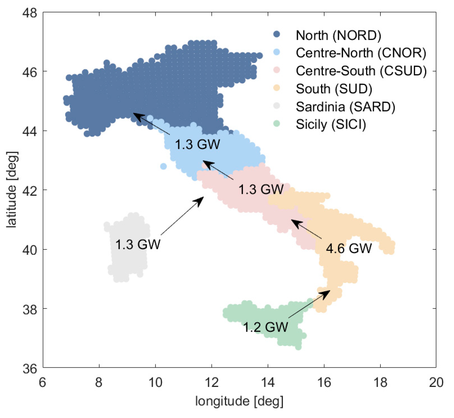
Until 2020, Italy was divided into six market zones (In 2021, the Italian TSO add another zone; therefore, currently, the country is divided into seven market areas.) defined by the Italian TSO according to national transmission grid constraints that limit the capacity transit between areas (Figure 1).
In this paper, we adopt the market zones nomenclature used by the Italian TSO: NORD (north zone), CNOR (center–north zone), CSUD (center–south zone), SUD (south zone), SICI (Sicily island) and SARD (Sardinia Island).
The imbalance between demand and supply in each market zones is defined as:
Δ P i m b = P s u p p l y s c h e d u l e d - P n e t l o a d = P n e t l o a d f o r - P n e t l o a d
where the netload (or residual load) is the electricity demand net of the solar and wind generation, while the generation scheduled for the next day (that will have to be supplied by dispatchable generators) is the netload day-ahead forecast.
P N e t l o a d = P l o a d P P V P w i n d
When the imbalance is negative (less scheduled supply than demand), upward regulation services are needed, while, when the imbalance is positive (more scheduled supply than demand), downward regulation services are required.
The imbalance is currently evaluated at each market zone only when the netload is greater than zero. Negative netload values mean VRE overgeneration that must be re-dispatched out of the zone (if transit limits at the point of interconnection allow) or curtailed.
Day-ahead netload forecast is used by the Italian TSO to size the tertiary reserve and ask, one day in advance, to the Balancing Service Providers the bids for load following and unit-commitment ancillary services. The great portion of Tertiary reserve (“Terziara di sostituzione”) is dimensioned by using a symmetric band (for up/downward regulation) evaluated through the 99.7% order quantile of the forecast errors [47]. Therefore, the maximum system flexibility (Tertiary reserve) required to resolve the imbalance related to incorrect demand scheduling can be defined by:
P f l e x i b i l i t y = Q 99.7 Δ P i m b
Evaluation of the imbalance ( Δ P i m b ) occurred over one year.
It is worth remarking that energy to balance the demand–scheduled supply is negotiated (one day ahead) on the Dispatching Services Market (MSD), while the energy to resolve imbalances due to contingency (unpredictable events) is acquired on the real-time Balancing Market (BM). Equations (1) and (3) refer only to energy exchanged on the Dispatching Services Market, and the MSD and flexibility requirements are related only to the flexible capacity need to compensate forecast errors that is approximatively half of the total imbalance volumes.

3. Methodology

The Italian imbalance volume and cost are defined as:
V o l u m e = h = 1 N h Δ P i m b h
C o s t = h = 1 N h [ δ h V M S D h + 1 δ h V M S D h ]   Δ P i m b h
where δ h   is a Boolean function that is equal to one if Δ P i m b > 0 or equal to zero otherwise, V M S D and V M S D   are the prices on the MSD of the energy for upward and downward regulation and N h is the number of hours of the evaluation period (usually months or year). The energy needed to accommodate the imbalances is purchased/sold by the Italian TSO on the energy markets (MSD and MB) using the “pay as bid”, scheme and the costs are mainly borne by the ratepayers.
Nowadays, the Italian imbalance volume and cost result from the sum of the zonal values. From Equations (1) and (3), it is clear that the simplest way to reduce imbalance and flexibility requirements is to improve the forecast accuracy by advanced forecasting methods. This is also the cheapest solution, since it can be done almost with no additional cost. The second way to reduce imbalance and flexibility is to remove the NTG bottleneck between the market zones enlarging the forecast-controlled area to the entire country. This will provide a further improvement of the prediction accuracy due to the “smoothing effect” (i.e., spatial decorrelation of the forecast error). This imbalance/flexibility mitigation measure requires significant investments, but most of them (8.9 billion EUR in the next 10 years [48]) are already planned, since the reinforcement of the national transmission grid will be essential for the RES transition: (1) enable the better distribution of VRE generation across the country, (2) allow for a better share of flexible resources and more efficient generation, (3) avoid congestions and the curtailment of VRE through redispatch of zonal VRE overgeneration and (4) enable the integration of energy markets.
The objective of this work is to quantify the margin of reduction of the imbalance and flexibility requirements (at current and future VRE penetration levels) that can be achieved in Italy by improving the accuracy of forecasts and enlarging the forecasting footprint to the entire country through NTG-strengthening projects.
For this aim, we adopted the following methodology:
We developed advanced forecasting methods for the day-ahead prediction of load and VRE generation in each market zone. We evaluated our forecasts by comparing with the most used baseline forecasts (persistence) and by comparing the volume and costs of the imbalance obtained from our advanced forecasting methods with those obtained from the Italian TSO during 2016 (test year).
We computed the imbalance/flexibility requirements of 2016 of each market zone and of all the possible areas obtained by unifying two or more adjacent market areas.
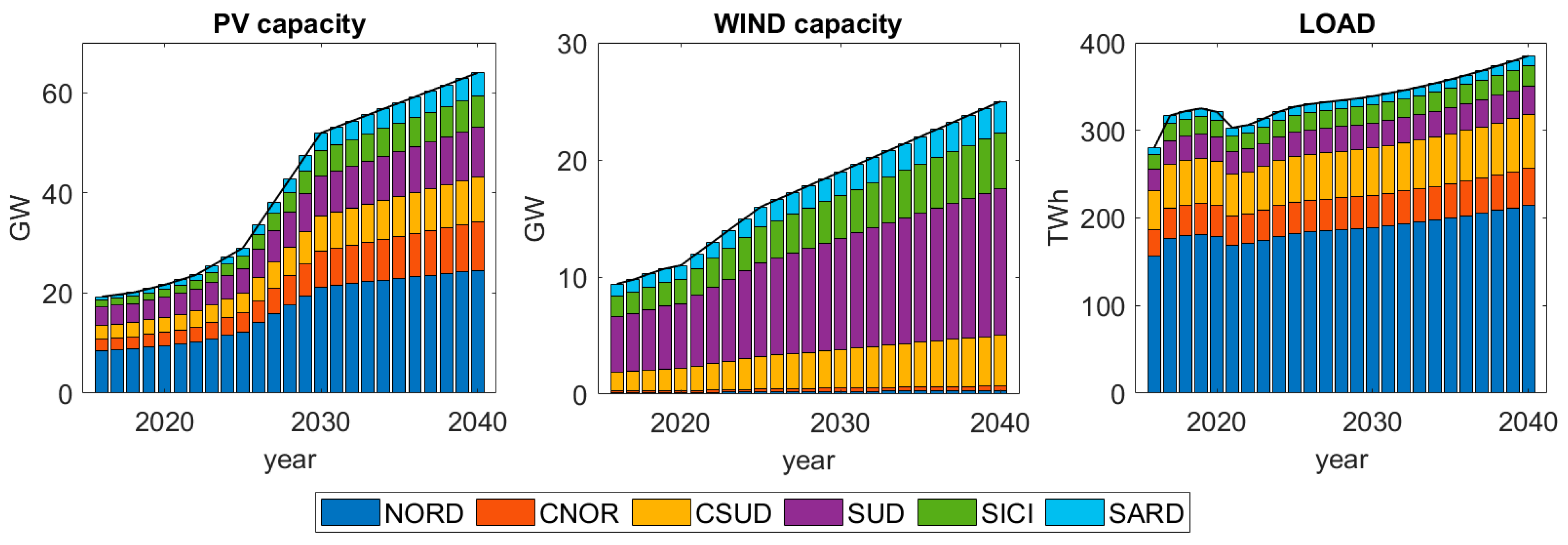
We used the load and VRE capacity growth scenarios (Figure 2) developed by the Italian TSO (according to the National Integrated Climate and Energy plan and “National Trend” European scenario published by ENTSO-E) to assess the order of magnitude of the imbalance/flexibility/overgeneration that could be achieved in the future using our forecasting methods on both individual market areas and a single national market.
For all the analysis and for the implementation of the neural network, we used MATLAB [49].
Figure 2. Load and VRE capacity growth NT-Italy scenarios developed by the Italian TSO [50].
Energies 15 09086 g002

4. Advanced Forecasting Methods

The available data used in this study provide the regional VRE fleet yearly installed capacity for each market zone, but they do not include information on their daily output variability, their physical characteristics and their geographical distribution. For this reason, we consider the regional VRE generation as if it was produced by virtual solar and wind power plants whose outputs are predicted using NWPs spatial aggregation.
In this section, we describe the load and VRE generation data applied to train/validate/test the methods (Section 4.1), the NWPs used as input of the forecasting models (Section 4.2) and the upscaling methods applied to predict the load and VRE generation of each market zone (Section 4.3).

4.1. Load and VRE Generation Data

We used a real Italian hourly load, PV and wind generation data and day-ahead and dispatching market price signals related to the years 2014–2016, and we assumed 2016 as the reference testing year. The data are public and downloadable from the Terna Spa website [51].
Table 1 shows the area of each market zone and the allocation between zones of the annual load and installed wind and solar capacity in the reference year.

4.2. Numerical Weather Prediction Data

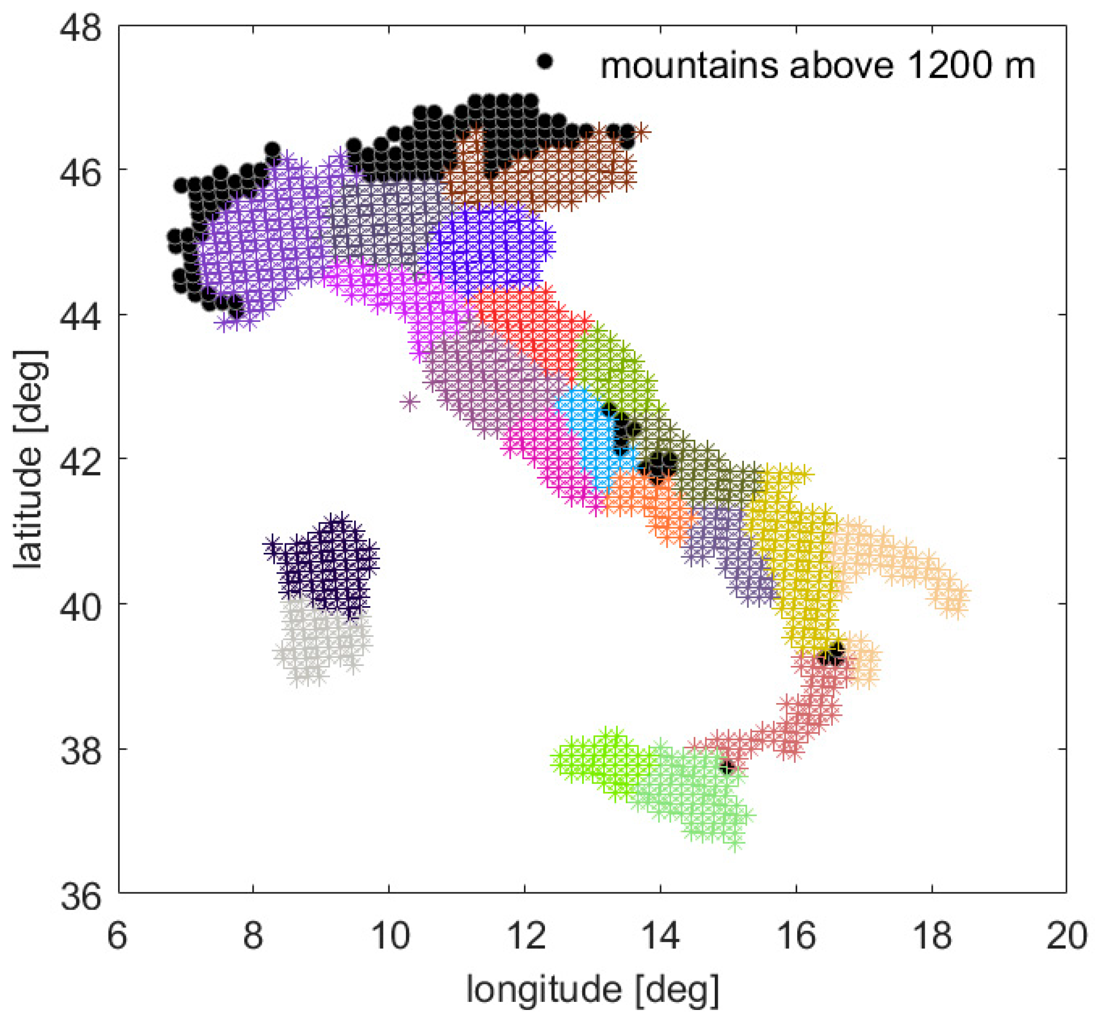
For the VRE power forecast, the time series of day-ahead prediction of global horizontal irradiance (GHI) air ground temperature (Tair) and wind speed were analyzed for three years (2014–2016) and 1325 locations covering the entire country with a spatial resolution of 12 × 12 km (Figure 3). The NWP forecasts were generated by the Weather Research and Forecasting model (WRF–ARW 3.8) [52] developed by the National Center of Atmospheric Research (NCAR). The model was initialized at 12 UTC, analyzing the 24-h forecasts starting from the following 00 UTC, which is the typical procedure for the day-ahead forecast:
Initial and boundary data for model initialization: GSF model output.
Radiation scheme: “Rapid Radiative Transfer Model”.
Forecast horizon: 24 h/temporal output resolution: 1 h/spatial resolution: 12 km.
The NWP irradiance data were also postprocessed, with an original Model Output Statistic based on an Artificial Neural Network model similar to the one developed in [53].
The NWPs were provided by the start-up company Ideam, a spinoff of Meteo Operations Italia (the largest private provider of meteorological services), currently in charge of providing national solar energy forecasts to the public company GSE that manages all the RES generation in Italy. For further information, Spena et al. [54] described in detail how to measure, analyze and collect solar radiation data.

4.3. Upscaling Methods to Predict Day-Ahead Load and PV/Wind Power Generation

In this subsection, we describe the method that we developed to predict the netload of each market zone according to Equation (2).
Before going into the details of the forecast models, it is important to spend few words on one of the problems of regional forecasting—that is, how to aggregate/select locations on which to calculate NWPs (In our case, all the 1325 grid points distributed across the nation). In fact, depending on the variable that is to be predicted and on the size of the region, the outperforming forecast method is achieved by ingesting NWP aggregated at different spatial levels (as for, example, Figure 3 in case of GHI NWP).
In contrast, to predict a demand, it is enough to use a simple zonal average of NWP weather data, since the load profile is driven primarily by user behaviors and only secondarily by weather conditions. In addition, at the zonal level, consumers can be considered uniformly distributed; thus, the regional average is a good predictor.
For PV power forecasting, to consider for the spatial variability, we had to use the NWPs of the irradiance averaged on specific clusters. We proved in [35] that the number of clusters to be used decreases as the size of the region increases. Indeed, since PV systems are widely distributed across the region, the higher the area controlled by the predictions, the more evenly distributed they appear so that the average irradiance becomes an increasingly good predictor. For wind power forecasting, by contrast, it was necessary to use NWPs of wind speed at high spatial resolution (12 × 12 km2). In fact, wind farms are not dispersed over the controlled area similar to solar power plants, so the data-driven forecast model must be able to select grid points where NWPs are most correlated with regional wind generation.

4.3.1. Day-Ahead Load Forecast

As mentioned above, the hourly profile of electricity demand (load) is driven by the statistical behavior of consumers, and only its daily value (integral over 24 h) is slightly influenced by the daily average temperature and irradiance, so it is much more predictable than VRE generation, which depends directly on the instantaneous variability of weather conditions.
Since the hourly load profile has an approximately weekly periodicity, and only the daily demand changes from week to week, the simplest but quite accurate load prediction can be obtained by a smart persistence model (SP) [55] that corrects the weekly persistence prediction with the mean daily bias error ( MBE ) of the persistence forecast of the current day:
P L o a d f o r S P t = P L o a d f o r P t M B E t 24  
where P L o a d f o r S P t is the prediction of the load of the smart persistence model, M B E t 24 = 1 24 t = 1 24 P L o a d f o r P t 24 P L o a d t 24 and P L o a d f o r P t = P L o a d t 24 x 7 is the weekly persistence forecast (i.e., load value of the same hour of 7 days before).
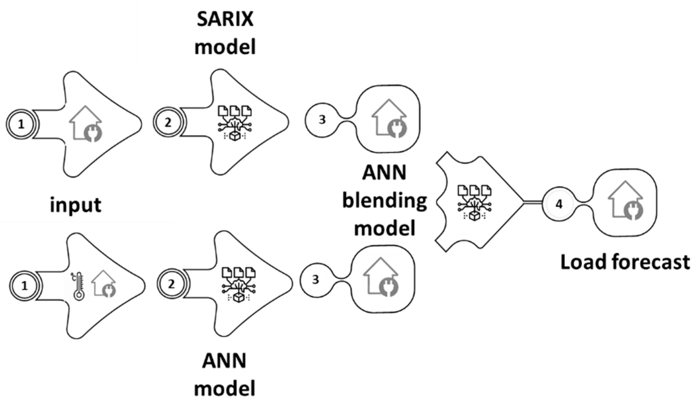
To improve such a simple prediction, we developed a forecast method based on the blending of two different predictions (Figure 4) obtained by a time series linear model and a MLP-ANN ensemble.
Time series linear models are a family of stochastic processes, namely seasonal Auto-Regressive Integrated Moving Average with exogenous inputs (SARIMAX), widely used to predict time–series signals. The selection of the best model that predicts the load profile is not trivial. As the load is nonstationary on average, has strong autocorrelation with lag 1 and shows a weekly seasonality, we chose the model S A R I 1 , 0 1 , 1 168 . Finally, because the smart persistence is a quite accurate prediction, we used it as exogenous input; therefore, the model becomes: S A R I X 1 , 0 1 , 1 168 :
1 ϕ 1 B 1 B 168 1 Φ 1 B 168 P L o a d f o r S A R I X t = γ   P L o a d f o r S P t + e t  
where B is the backshift operator; ϕ 1 , Φ 1 and γ are the coefficients of the autoregression; e is the expected forecast error (white noise) and P L o a d f o r S P is the smart persistence forecast. Model coefficients are retrieved each day using the load values of the previous 30 days (moving window).
The MLP-ANN ensemble basically corrects the smart persistence prediction by taking into account daily weather conditions:
P L o a d f o r A N N t | X ^ = f 2 W 2 f 1 W 1 X + b 1 + b 2  
where (i = 1, 2) is the layer index, and f i are hyperbolic and linear transfer functions; W i and b i are the empirical parameter retrieved by the training and validation procedures, and the input X are the daily average of the predicted air temperature and irradiance and the smart persistence forecast.
Finally, the further accuracy improvement with respect to the smart persistence was obtained blending the two forecasts by another ensemble of MLP-ANN:
P L o a d f o r A N N   b l e n d t | X ^ = f 2 W 2 f 1 W 1 X + b 1 + b 2  
In this case, the input X are the month, the weekday and the SARIX and ANN load predictions.

4.3.2. Day-Ahead PV Power Forecast

PV power prediction was obtained by an upscaling method based on a hybrid forecasting model, such as the one described in [36,56] for all of Italy. Additionally, in this case, data pre/postprocessing are essential to obtain accurate predictions.
The inputs of the method are the NWP of the global horizontal irradiance (GHI), the air temperature at 2 m (Tair) and the solar elevation (sunEL) computed to all the grid point of each market zone.
The preprocessing of the training year data consists of: (i) clustering the 1325 GHI time series (satellite retrieved) of the training year in 20 subregions with similar irradiance (Figure 3), (ii) compute the spatial average of the NWPs all over the market zone and (iii) retrieve the best tilt and orientation angles of the regional VPP (“equivalent“ plane of the array -POA-) by minimizing the errors between the PV power rate estimate by a deterministic model and the solar generation rate of each market zone (provided by the TSO). The deterministic model is a semi-empirical physical-based model [53] that maps the GHI, Tair and the angle of incidence (AOI) on the equivalent POA into the regional PV generation rate:
Y P V D M = f P V D M A O I ,   G H I , T a i r  
where the power rate is defined as Y P V = P P V / P n P V with P P V , P n P V being the solar generation and the solar-installed capacity.
Once the angles of the “equivalent” POA have been identified, the deterministic model was applied to the spatial average of the NWPs ( G H I f o r   and   T a i r f o r ) to get the first PV power rate forecast ( Y P V f o r D M ). The deterministic forecast is affected by strong bias on a daily time scale, probably due the assumption of a unique POA of the VPP, TSO power output estimation errors, uncertainty in the installed capacity (on monthly time scale) and PV performance degradation (on a yearly timescale).
Post-processing calculations aims to partially correct these biases with a daily performance factor (PRF) computed using the predicted and observed power values of the previous Nd = 15 days:
P R F f o r d d   |   P P V f o r D M = 1 Nd d d = 1 Nd t = 1 24 P P V ( t |   d d dd ) t = 1 24 P P V f o r D M ( t |   d d dd )
where d d is the day to be predicted, P P V ( t |   d d d d )   and P P V f o r D M ( t |   d d d d ) = P n P V d d   Y P V f o r DM ( t |   d d d d ) are the observed and deterministic prediction at the hour t of the day d d d d .
Afterward, P R F f o r and the deterministic model was used to calculate the PV clear sky ( P P V C S )   and the PV clear sky index ( K P V ) :
P P V C S = P n P V P R F f o r   f P V D M A O I ,   G H I c s ,   T a i r f o r      
K P V = P P V   / P P V C S  
where G H I c s and T a i r f o r are the clear sky irradiance and ground air temperature forecast averaged over the entire market zone, while AOI is the angle of incidence on the zonal “equivalent” POA.
K P V is stationary both in mean and in variance and can be predicted by an ensemble of MLP-ANN models:
K P V f o r A N N t | X ^ = f 2 W 2 f 1 W 1 X + b 1 + b 2  
where, in this case, the input X are the clear sky indexes averaged on the points of the irradiance clusters (Figure 3) belonging to the specific market zones ( K C S f o r c l u s t e r = G H I f o r c l u s t e r / G H I C S c l u s t e r ), the zonal average of sun elevation( s u n E l ) and the air temperature forecast ( T a i r f o r ).
Finally, the prediction of PV generation on each market area is obtained by:
P P V f o r   A N N = P n P V Y PV for ANN = K P V f o r A N N P P V C S  
The forecast process is summarized in Figure 5.
Dissimilar to the DM model that ingest the irradiance averaged all over the regions, the ANN model considers the nonuniformity of the irradiance and PV capacity distribution inside the forecast-controlled area through the K C S f o r c l u s t e r spatial variability.

4.3.3. Day-Ahead Wind Power Forecast

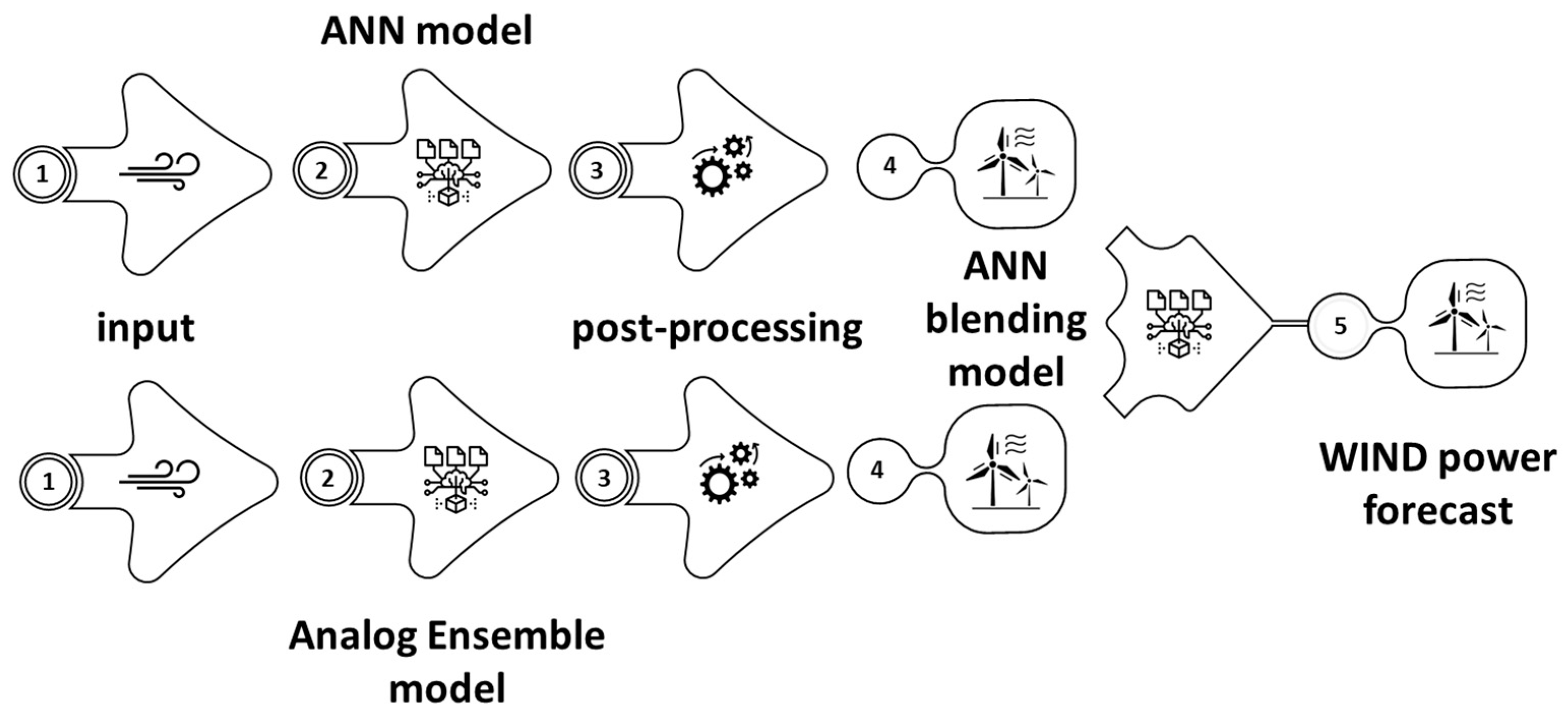
Wind generation forecast was obtained by a blending of the predictions generated by two different upscaling methods (Figure 6).
Both the methods use as input the wind speed predicted on all the grid point inside each market zone.
The forecast model of the first methods is a qualify ensemble sorted by 20 predictions generated by a multilayer perceptron with one hidden layer (ANN model):
Y W i n d f o r A N N t | X ^ = f 2 W 2 f 1 W 1 X + b 1 + b 2  
where X ^ are the input: wind speed perditions. P W i n d is the wind power, P n W i n d is the regional wind installed capacity and Y W i n d = P W i n d / P n W i n d is the wind power rate.
It is worth remarking that, to consider the wind speed cut-in of the turbines, during the training phase, all the generation data for which was predicted an average wind speed below 2 m/h was set to zero. Therefore, also in this case, the use of preprocessing in the training phase was essential to eliminate the forecast bias at a low wind speed.
The forecast model of the second method is an Analog Ensemble (AE), i.e., a statistical method based on the assumptions that similar NWP input should correspond to similar power outputs (definitely true if the correct NWP variables underlying wind generation have been included in the input and if the NWP model generating these variables has not been modified) [57]. Therefore, first, a set of past predictors most similar to those of the hour to be predicted is selected via a similarity metric; then, the real power generation data corresponding to the selected set of past predictors is used as a deterministic/probabilistic forecast. In this case, we defined the similarity metric as:
d W t , t = p = 1 N p W p || X F ^ p , t X ^ p , t ||
where p represents each type of predictor, X F ^ p , t is a vector containing the current forecast (at time t) of the p th predictor type (normalized by min/max values of the historical data set), X ^ p , t is the normalized past forecasts vector (at past time t’) of the bbbbb predictor p and W p are the optimal weights associated to each predictor type ( p W p = 1 ). In this case, the predictors ( X ^   and F X ^ ) are the wind speed forecasts on all the grid points of the area; therefore, p = 1 and W p =1.
At each time t, the first 25 analogs which have the lowest distance d W are selected among the predictions of previous 30 days, and then, the power rate forecast is computed as:
Y W i n d f o r A E ( t | X ^ ) = 1 25   i = 1 25 b n P w i n d ( t i   | d W t , t i ) / P n W i n d t i
where b 1 = 0.2 for the minimum distance and b n = 1 b 1 / 24 for the other 24 sub-minima distances.
Both ANN and AE forecasts were affected by bias errors dependent on the predicted generation values that were corrected by a post-processing procedure. Post-processing computes a performance factor ( P R F ) using the forecast and observed power values of the previous N d = 15 days, according to 5 different intervals of wind power rate predictions ( Y W i n d f o r ):
P R F W i n d f o r ( t   |   Y W i n d f o r ϵ   i n t ) = t = t 24 * N d t 24 Y W i n d   t |   Y W i n d f o r ϵ   i n t / t = t 24 * N d t 24 Y W i n d f o r   t |   Y W i n d f o r ϵ   i n t
where i n t = 0 0.2 ,   0.2 0.4 , 0.8 1 .
Thus, the power rate prediction is:
Y W i n d f o r A N N + P R F = P R F W i n d f o r * Y W i n d f o r A N N
Y W i n d f o r A E + P R F = P R F W i n d f o r * Y W i n d f o r A E
The final day-ahead prediction of the regional wind power rate was obtained by blending the two forecasts reported in Equations (20) and (21). The used blending technique is again a qualified ensemble of multilayers perceptron so that:
Y W i n d f o r A N N   b l e n d t | X ^ = f 2 W 2 f 1 W 1 X + b 1 + b 2  
where the input X are the two previously described forecast ( Y W i n d , o r A N N + P R F and Y W i n d o r A E + P R F ).
Finally, the prediction of wind generation on each market area is obtained by:
P w i n d f o r   A N N   b l e n d = P n W i n d   Y wind for A N N   b l e n d
The forecast method is summarized in Figure 6.

5. Metrics

Table 2 reports the prevailing metrics used in the literature to evaluate the forecast accuracy, where X is the variable that should be predicted and X n is the PV/wind installed capacity or the peak load, while n h is the number of the yearly hours for the load and wind predictions and is the number of yearly daylight hours for PV power forecast.
Following the use of TSOs, the RMSE, MAE and MBE are all expressed as a percentage of the installed PV/wind capacity or peak load. In research on forecasting PV and wind energy at the regional level, the most widely used benchmark model for assessing the Skill Score is the persistence model: P W i n d / P V f o r P t = P W i n d / P V t 24 . In the case of load forecasting, to better assess the forecast improvement, we used as the benchmark model the smart persistence defined in Equation (6).

6. Results

In this section, we present and discuss the results obtained. In Section 6.1, we evaluate the accuracy of our load/PV/wind forecasts compared to the accuracy of the reference models. In Section 6.2, we validate our forecasts by comparing the imbalance volume and costs resulting from our forecasts with the real imbalance volume/costs resulting from netload forecast method developed by the Italian TSO. In Section 6.3, we show the margins for reducing imbalances and flexibility requirements that can be achieved with our netload forecast compared to those achievable with the persistence baseline forecast, both at the market area and country level. In Section 6.4, we estimate the imbalance volumes/costs/flexibility and VRE overgeneration that may occur in the future according to the NT scenario.

6.1. Day-Ahead Forecast Accuracy Evaluation (Test Year 2016)

6.1.1. PV Forecast Accuracy

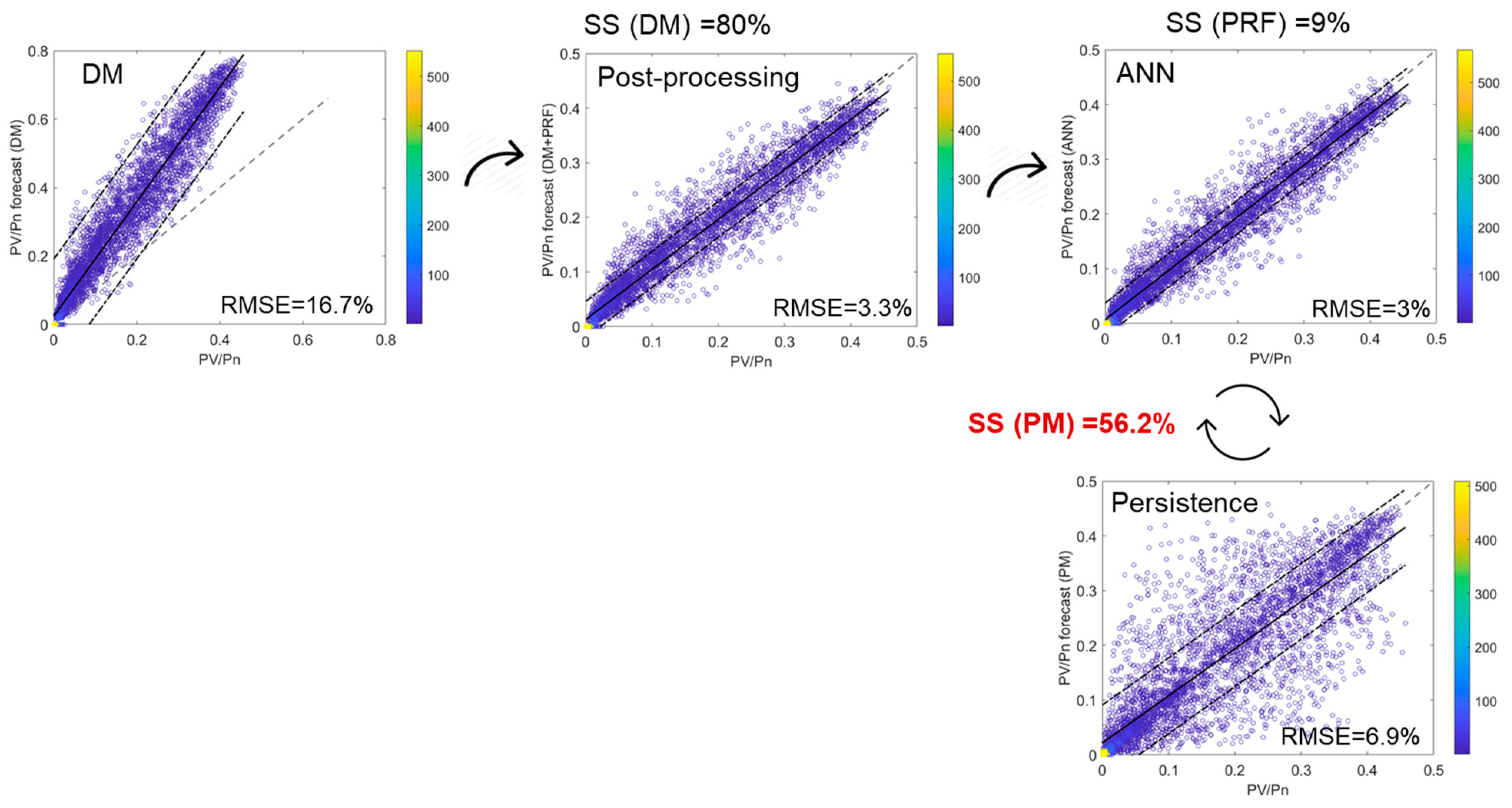
Figure 7 reports, for the northern zone, the scatterplots (observations vs. predictions) of the model chains that make up the hybrid method used for solar energy forecast together with the scatterplot of the persistence model.
The deterministic model provides a strong systematic over-prediction that was corrected by post-processing the prediction errors of the 15 days prior to the day to be predicted, resulting in an 80% improvement in accuracy. The ANN model, which considers the non-uniformity of irradiance and PV capacity along the region, reduces the out layers achieving an additional 9% of accuracy improvement.
At the end of the process, we obtain 56% of skill score with respect the persistence prediction.
Table 3 summarizes the main performance indicators of the forecast for the six Italian macro-regions. For each of them, the regional area is given in the first column. For all regions, the correlation is between 0.95 and 0.97. MBE is very small (as expected) ranging between 0.001% and −0.003%. The MAE is between 2.1% and 3.4%. The RMSE of our forecast (ANN hybrid model) is in the interval between 3.0% and 5.0%, while the RMSE of the persistence forecast (PM) is between 6.9% and 9.4%. The values for rhe Skill Score (SS) range from 48.3 to 56.1 for all regions except CNOR, where the SS = 36.3%.
The regional PV forecast accuracy depends on the persistence of the weather conditions and of the size of the forecast-controlled area. The more the irradiance profile does not change from day to day (low day-ahead variability), the lower the RMSE of the persistence prediction and thus the easier the day-ahead PV generation is to predict. Therefore, RMSE of the persistence model gives an indication of weather variability/predictability. On the other hand, increasing the size of the forecast-controlled area, due to the stochastic behavior of weather conditions, the spatial variability is increasing smoothed as well as the forecast errors from one side to the other of the region are more and more decorrelated thus they decrease in spatial average. Therefore, the larger the area controlled by the forecasts, the easier the predictability of the regional PV generation (with smoothed profile) and the more accurate the forecasts are. This is call “forecast smoothing effect”.
Wentz et al. [58] compared two machine learning methods: Artificial Neural Networks (ANN) and Long-Term Short Memory (LTSM); they found that in very short prediction (1, 15, 60 min) LSTM outperform ANN. Dolara et al. [59] used an hybrid model and an ANN method for predicting solar radiation and they found that the hybrid method is more accurate than just the ANN even changing some settings in the neural network. A weather classification approach with support vector machine is used in the work of Shi et al. [60] Their Mean Relative Error (MRE) range from 12.42% to 4.85%, respectively, for cloudy and sunny models, which is definitively higher than our case, probably because of a shorter time series available. Conversely to the above-mentioned results, our approach is based on combining different models, from physical to machine learning, to maximize the ability of each model to improve the accuracy in forecasting solar radiation. This cascade approach results in a decrease of the uncertainties.
From Table 3, it can be seen that the RMSE of the northern zone (three to four times larger in size than the other regions), is 1/3 lower than the average RMSE of the other zones (3% compared to 4.5% on average) We can also see that with the exception of the CNOR zone, comparing regions of similar size, the lower the RMSE of persistence the lower the RMSE of our prediction (for instance SARD vs. SICI).
Figure 8 show, by way of example, the hourly values of observed and predicted PV for three days in March 2016, the 3rd, 4th and 5th in the north zone. Interestingly, although the three days have different weather conditions (variable, clear and overcast) due to the large size of the region, the PV generation profiles are all very smooth.

6.1.2. Wind Forecast Accuracy

When we take wind energy into account, both the accuracy of the models and the precision decrease significantly comparing to solar prediction. The reasons for this lie in the nature of the source: wind energy production is much more variable and site dependent than solar. Furthermore, wind farms are not as distributed along regions as solar plants, so forecasting wind generation at the regional level would require more precise information on the location of individual plants. Finally, the distribution of wind speed affects production in nonlinear way with a cut-off and cut-in at high and very low speeds while PV generation is approximatively proportional to the incident irradiance. Therefore, small errors in the NWP of wind speed or uncertainty about wind power plant technology could have a much greater impact on the accuracy of wind generation prediction. In this case, forecasting regional wind generation was extremely challenging because we have no information on either the location or technology of the wind farms, but only know the aggregate output and annual installed capacity.
To predict wind power generation, we optimally blend the results of two upscaling methods based on Analog Ensemble (AE) and Artificial Neural Network (ANN) models, respectively.
Figure 9 reports, for the southern zone, the scatterplots (observations vs. predictions) of each step of the forecast methodology along with the scatterplot of the persistence model. The AE and ANN models provides a systematic under-prediction that was corrected by a post-processing procedure. It is worth noting that while post-processing removes bias, it does not necessarily improve accuracy in terms of RMSE; in fact, the RMSE of the post-processed AE output decreases by 2.5%, while the RMSE of the post-processed ANN output increases by 8%. However, unbiased predictions are essential to build an ANN blending model that has the ability to optimize the outliers and good results of each approach. The optimal blending improves the accuracy the AE and ANN upscaling methods of 27% and 19%, respectively, reaching a skill score over the persistence forecast of 53%. The improvement obtained with this blending approach is highly significant, even without considering all variability effects associated with the wind source.
As summarized in Table 4, the correlation for wind energy is still high, ranging from 0.81 to 0.87 for all regions, MBE ranges from 0.003% to 0.015%, MAE ranges from 6.0% to 8.1%, RMSE ranges from 8.5% to 12.2%, while RMSE of persistence forecast ranges from 18.1% to 22.4%. The values of SS range from 45.4% to 53.8% with an average value of 48.7%.
First, it should be noted that the RMSE of our wind forecast compared with the one of the PV predictions is more than two time higher (9.2% vs. 4.2% in average). On the other hand, the RMSE of the wind persistence prediction is also more than twice as high as the RMSE of the PV persistence (18.2% vs. 8.3%), indicating the higher variability of wind speed than irradiance (as mentioned above).
The fact that the skill scores of the wind and PV are almost equal (on average: 48.7% vs. 48.8%) means that the two forecasting methods have the same forecasting ability, but the greater variability of the resource underlying the generation decreases the accuracy of the forecast.
Secondly, we point out that, due to the stochastic variability of the resource, also predictions of regional wind generation such as those of solar benefits of the “smoothing effect” (increase of forecast accuracy as the size of the region increases). Indeed, also in this case, the RMSE of the wind prediction of the northern zone is less than half of the average RMSE of the forecast of the all-other zones (4% vs. 10.2%).
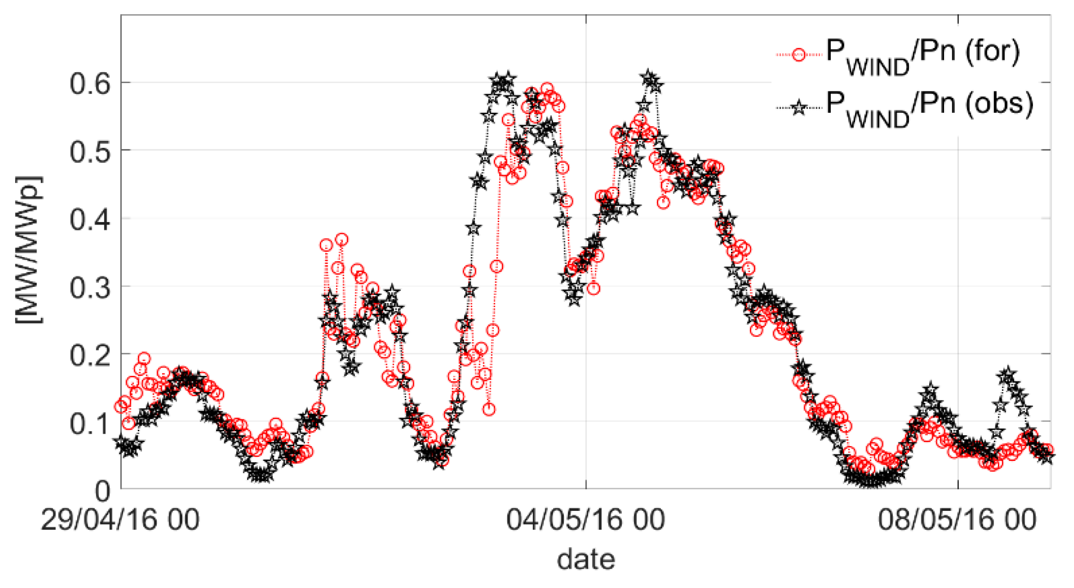
Figure 10 shows, by way of example, the hourly values of observed and predicted wind generation for seven days of 2016: from 30 April–5 March in the South zone. Looking at both Figure 8 and Figure 10, we can see the greater hourly variability of wind generation compared to solar and the greater difficulties in forecasting.

6.1.3. Load Forecast Accuracy

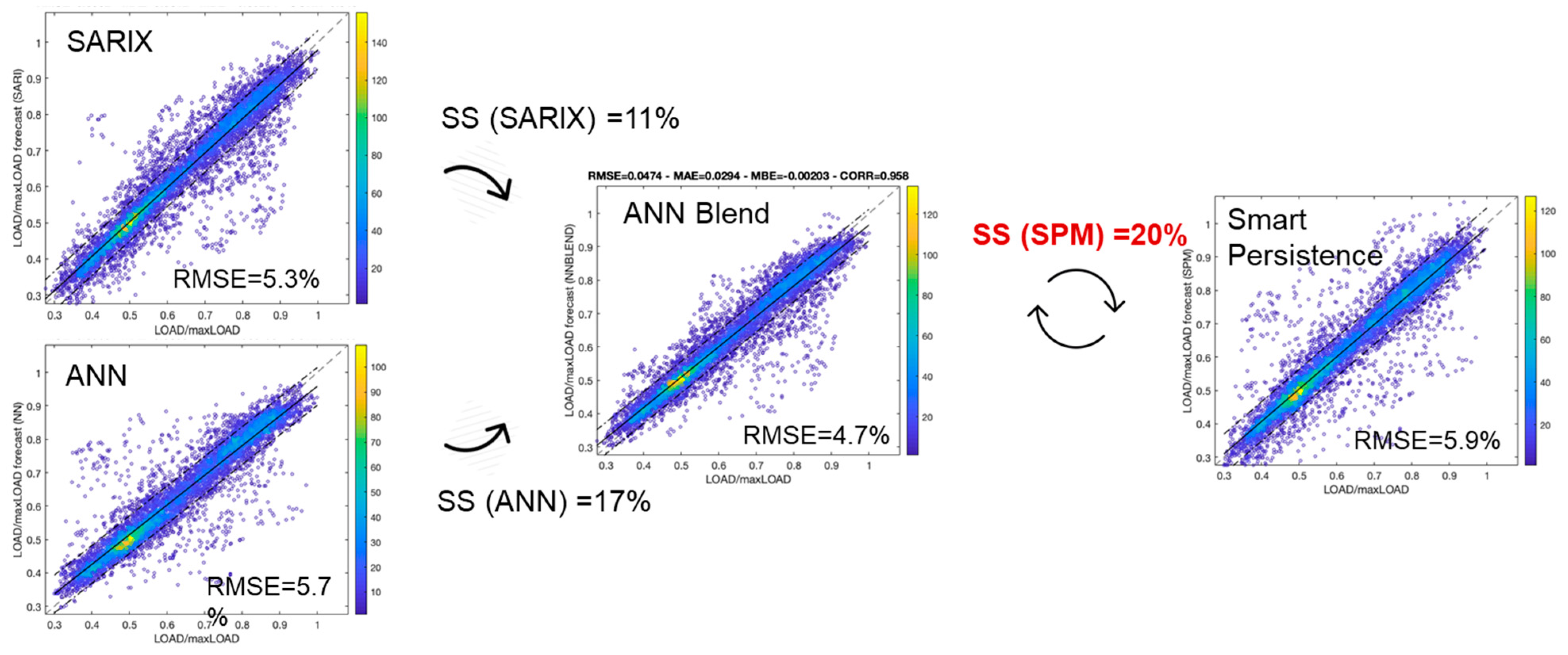
Figure 11 shows the scatterplots (observations against forecasts) of SARIX and ANN predictions, of the ANN blend and of the smart persistence forecast for the Northern zone (which is the one with higher electric demand). It also reports the accuracy and the skill score of the various forecasting methods. We can see the advantage of using the blending method over the individual predictions (11% and 17%) and the improvement in accuracy over the smart persistence prediction (20%).
Table 5 shows, for the six market zones, the values of the accuracy metrics of our ANN blend forecast, the RMSE of the smart persistence prediction and the skill score over this reference model: correlation ranges between 0.92 and 0.97, MBE between −0.004% and 0.003%, MAE between 2.2% and 3.4%, RMSE between 3.2% and 4.9% while RMSE of the smart persistence ranges between 3.8% and 5.9% and SS between 17% and 21.3%. These values do not differ too much between market zones, and the RMSE of the North zone is even higher than the average RMSE of the other regions (4.7% vs. 3.8%). This is because, dissimilar to solar and wind, the load depends mainly on the statistic behavior of consumers therefore the load profiles do not smooth when the forecast-controlled area increases as well as the errors in the prediction are always strongly correlated inside the area so that the forecast accuracy does not decrease with the increasing of forecast footprint.
It is worth noting that the SP statistical model provides a fairly accurate prediction, which is why, compared with the solar and wind skill scores, our forecast has a moderate improvement in accuracy over the baseline forecast (17.8% on average).
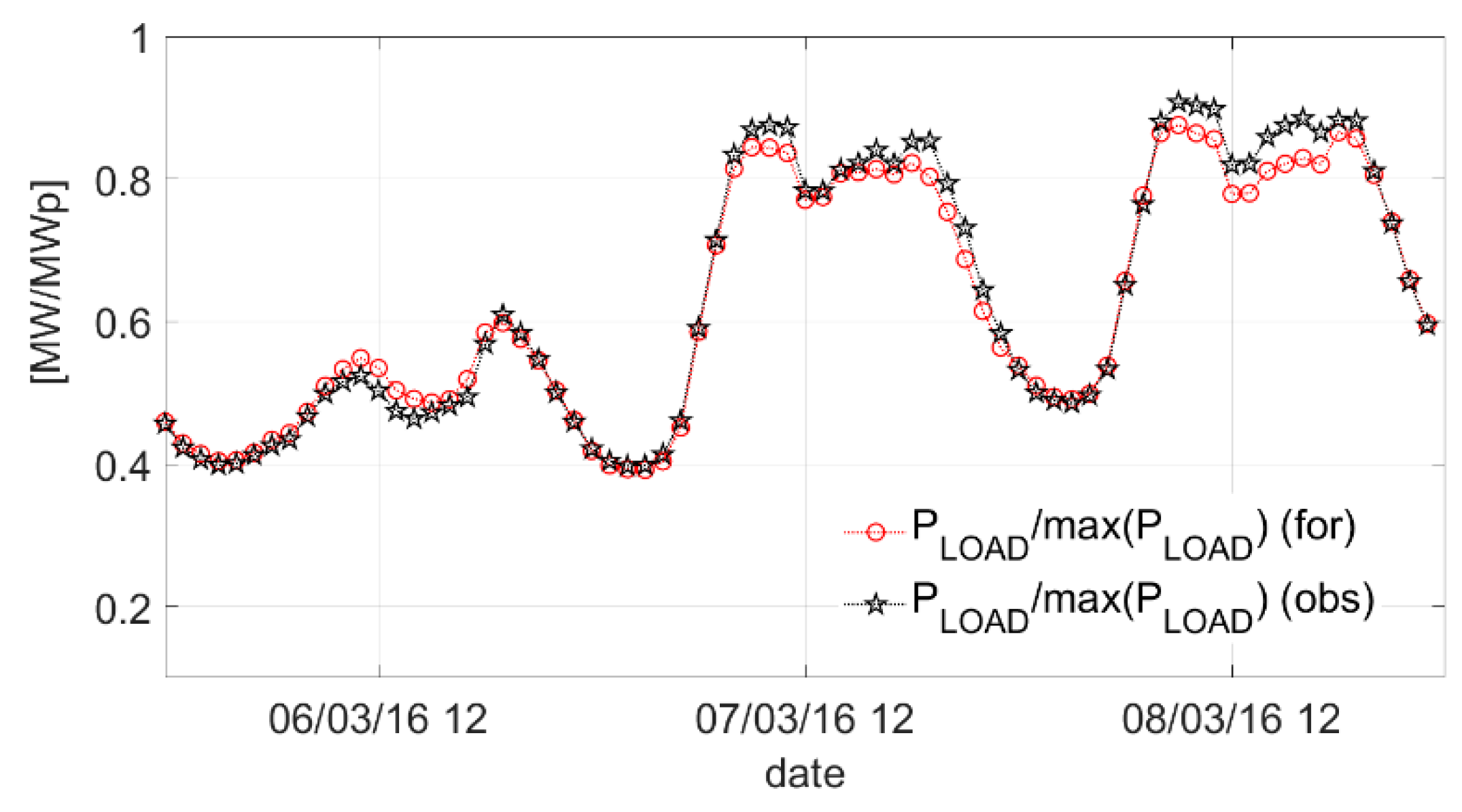
Figure 12 shows, by way of example, the time series of the observed/predicted load for the interval between 5 and 9 March 2016.
We also remark that the greatest forecast errors are related to the prediction of vacation days (which differ greatly from those of the previous week), by using a separate forecast method for these days it would surely be possible to greatly improve the load forecast accuracy.

6.2. Netload Forecast Accuracy Assessment and Validation

While we already proved that our PV generation forecast is at the “state of the art” level by comparing to other predictions (on a different test year) and with other results in literature [35], this is more difficult for wind. The ongoing wind forecast research is focused on the prediction of the generation of a single turbine or farm [61], thus, obtained accuracy cannot be directly compared the regional ones. Indeed, regional wind forecasts suffer from the lack of geographical/technical information on the wind fleet, but benefit from the smoothing effect. The main effort on this issue, however, is to reduce forecasting errors using different approaches. Louka et al. [62] and Lima [63] are both working to improve weather forecasting by applying a Kalman filtering method to both the input data and the systematic errors, resulting in a reduction of the RMSE. The combination of adaptive methods and integrated approaches improves the estimation of wind energy production, as presented by Vaccaro [64] who combined different data sources using a supervised learning system that merged data from different sources, such as wind speed observations in Italy and models. Similarly, Pang et al. [65] combined physical models and ANN approaches to achieve an 80% reduction in RMSE, which is higher than our results (about 53% for wind), but for individual power plants rather than a regional assessment as we did. To improve wind power plant load prediction De Giorgi et al. [66] included more atmospheric variables and different ANNs demonstrating the importance of considering the surface pressure and temperature in the plant site. With a comparable approach Velazquez [67] demonstrated the importance of wind direction as input of the ANN models to decrease the forecasting error of about 20%.
For load forecasting, there are not standard way for performance evaluation as in solar and wind, therefore accuracy in not normalize by the peak demand, different KPIs or evaluation period are used etc. [68], so that benchmark our method is very difficult.
For these reasons, we decide to assess the quality of our prediction directly comparing the imbalance volume and cost obtained by our netload forecast with the 2016 values resulting from netload prediction of the Italian TSO (Figure 13).
Figure 13a contains the values for the total downward and upward imbalance in the six Italian market zones (grey and black histograms, respectively) and the associated downward and upward prices (grey and black dots, respectively) [69]. Figure 13b shows the same values but applying the advanced forecasting approach we developed. Comparing the two figure an overall decrease in volumes and costs is observed with an annual reduction of 8% and 38%, respectively. It is worth noting that the TSO systematically slightly under-predicts residual demand, as upward regulation volumes are always larger than downward ones, which explains why we achieve 38% cost savings with 8% accuracy improvement (upward energy prices are much higher than downward). To be fair, given that in the real-time (MB) balancing market, the TSO has acquired more downward than upward regulation services, it is likely that the under-prediction is intentionally dictated to purchase in advance more upward reserves on MSD than real-time upward services on MB (which could be much more expensive). However, our prediction methods can be considered “state of the art” and compete in accuracy with current TSO prediction techniques.
In addition, Figure 13b shows that, if capacity transit constraints between market zones were removed allowing direct forecasting of the entire Italian VRE generation, our forecasting methods would have resulted in a reduction of imbalance volumes and costs by 33% and 54% respectively. Therefore, upgrading the national transmission grid to remove transmission bottlenecks between market areas not only allows current reserves to be used regardless of the area in which they are located (increasing the effectiveness of regulation), but also, due to the VRE “smoothing effect,” greatly reduces the volumes and costs of imbalance.

6.3. Margins of Reduction of Imbalance and Flexibility Requirements Due to Advanced Forecasting and NTG Reinforcement

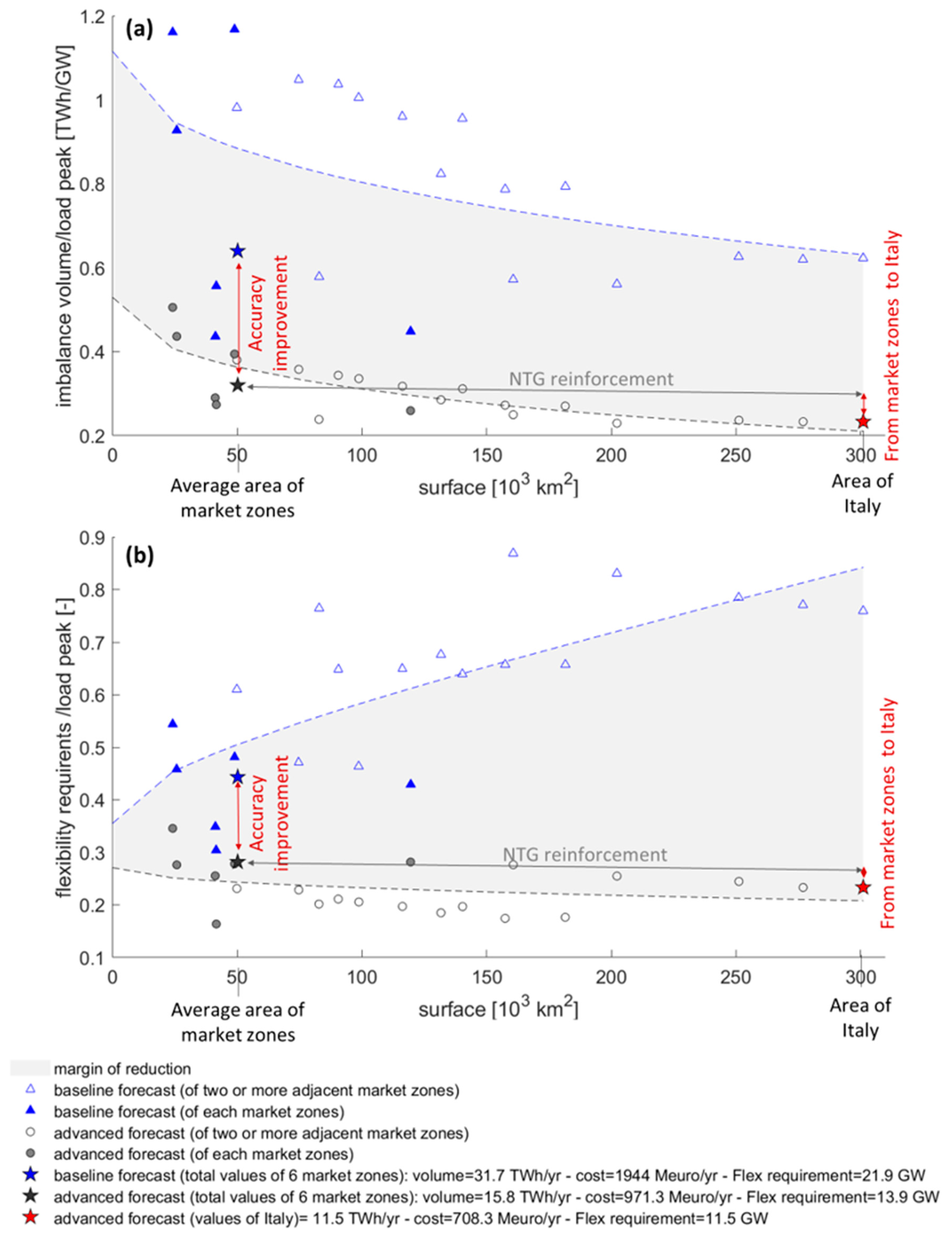
Figure 14 depicts the improvement our prediction achieves in terms of imbalance and flexibility for all 6 zones, the different combinations of two or more adjacent zones and the whole country. The x-axis shows the area of the different zones in km2 and to the right of it the total area of Italy. On the y-axis we give the values for imbalance volumes (Figure 14a) and flexibility requirement (Figure 14b). Colors indicate the forecast methodology: blue is for the simple persistence model while black is for our advanced forecasting methods. The blue/black stars represent the Italian imbalance volume resulting from the sum of the imbalances obtained from the netload prediction of each market zone.; red star is the Italian imbalance resulting from a single netload prediction at national level.
Figure 14a reveals that, by using the advanced forecast (black star) instead of the baseline forecast (blue star), the Italian imbalance would be reduced by 50%, while an additional 30% reduction could be achieved by removing NTG constraints between market areas (red star).
However, the results reported above show that the TSO has already reached a netload forecast accuracy near to the “state of the art level” (we obtained just 8% of imbalance reduction) while there is more room for imbalance reduction if advanced forecast is coupled with network strengthening measures (33% of imbalance reduction). Indeed, Italian TSO has already planned to enhancing trade between market areas for improve integration of renewable energy sources [49].
Figure 14b shows that, if the persistence prediction is used, smoothing effect is not enough to reduce flexibility when the forecast-controlled area increases. This means that although annual imbalance volumes decrease as the forecast footprint increases, this is not the case for the maximum forecast error when using very low-quality prediction (as the persistence model). In contrast, our forecast reduces the flexibility requirement by 38% compared to the value obtained through the persistence model, while reinforcement of the NTG could provide an additional 18% reduction.
These results are obviously dependent on regional weather conditions, so this analysis could be repeated for other countries, helping TSOs quantify the imbalance/flexibility benefits that can be achieved through forecast accuracy and transmission grid improvements.

6.4. Future Scenario of RES Penetration

Using the load/VRE hourly profiles of 2016 and our forecasting methods, we estimated the order of magnitude of imbalance volumes/costs/flexibility/overgenerations that could be reached in future according to load/VRE capacities growth scenario developed by the Italian TSO (Figure 2).
Figure 15 presents the future scenarios for the imbalance volumes (a) and costs (b) from now to 2040. Due to the increasing VRE penetration, the imbalance volume is expected to grow from the 17.7 TWh/y by 2021 to 21.3–24.9 TWh/y by 2030–2040 (+21% and +40%). This increase can be contained if it would be possible to enlarge the forecast footprint to the entire nation. In this case by 2030 we could have an imbalance of 16.3 TWh/y even lower than 2021 value, while by 2040 of 19.8 TWh/y (+12%).
The imbalance costs on the dispatching market (MSD), under the business-as-usual assumption and without considering the price impact of unexpected events such as the current Ukraine war, are expected to increase of 23–43% by 2030–2040 with respect the 1090 million euro calculated for the current year. We estimated that NTG strengthening measures aimed at market integration could reduce MSD imbalance costs (borne by ratepayers) by 350–400 million euros per year and even greater additional savings could come from reducing the cost of real-time balancing (MB) where upward regulation can reach incredibly high prices.
In addition, markets integration leads to a better share of flexible resources present in the country reducing the systems flexibility requirements. Therefore, other economic save arises from reduction of the auctions on the capacity markets that in Italy are indirectly funding the construction of new 42 GW thermoelectric reserves.
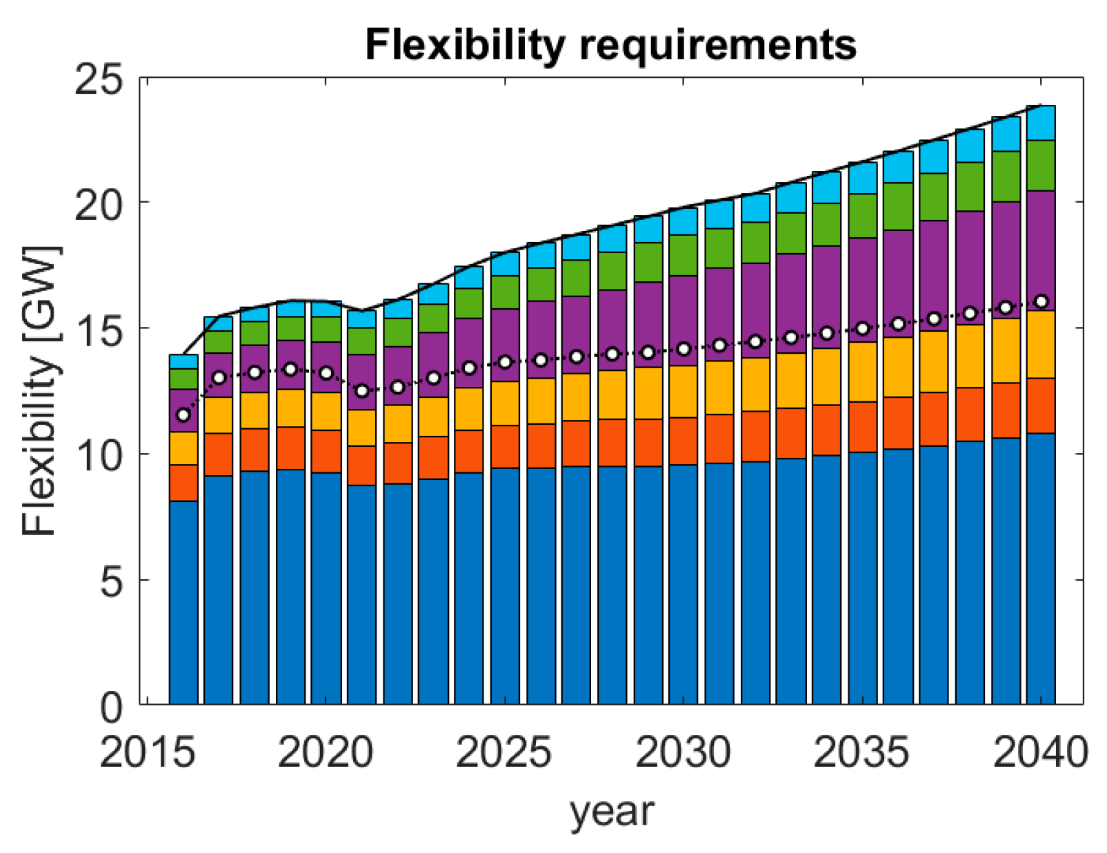
Figure 16 shows that, only for balancing residual demand and scheduled supply, an increase of system flexibility requirements of 27–53% will be needed by 2030–2040: from the current 15.6 GW of tertiary reserves to 19.8–24 GW. Market zones integration would almost entirely avoid the need to increase reserves for load-following and unit commitment ancillary services, as we estimate a flexibility requirement of 14.2 GW by 2030 and 16 GW by 2040.
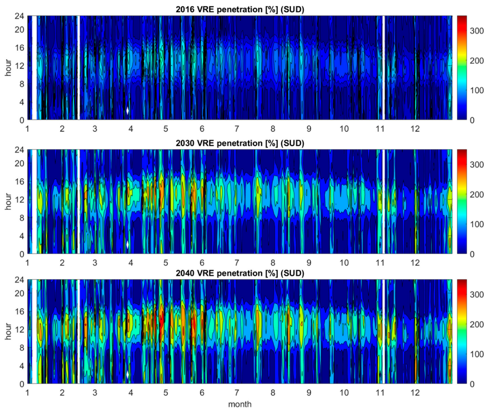
With the growing VRE penetration, the events during which wind and solar produce more than demand increase. Excess energy produced must be re-dispatched outside the market zone or curtailed when transit limits between zones are violated. This means that overgeneration implies reverse power flow events, as well as possible grid congestions.
Figure 17 shows the ratio between VRE production and the demand (VRE hourly penetration) of the southern zone. In 2016, there have already been instances where wind and solar generated more than 100% of demand (mainly during Sundays), but in 2030 and 2040 the number of such events will grow greatly, with VRE generation summer peaks of more than 200% and 300% of demand.
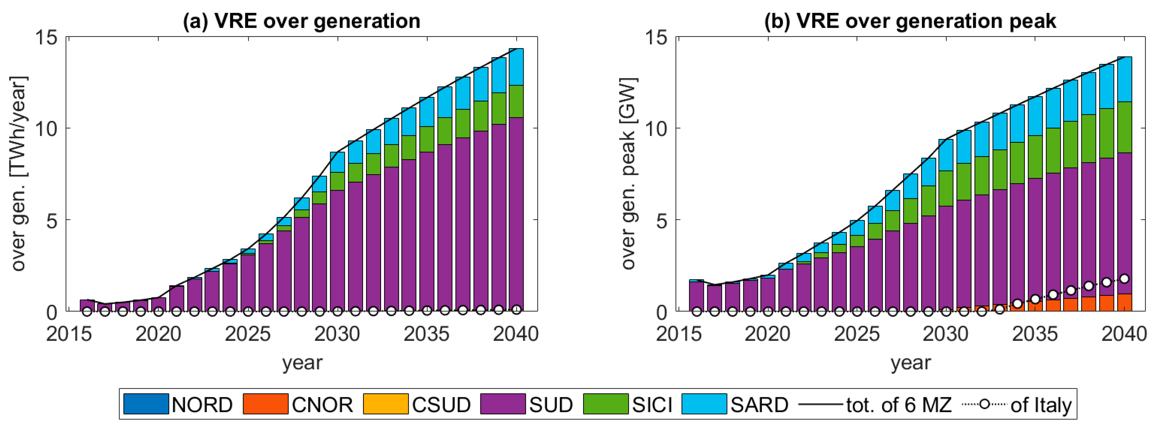
Figure 18a estimates the zonal/national VRE overgenerated energy according to the TSO scenario. It appears that the overproduction of VRE must be redistributed from southern and island areas and, in the absence of grid congestions, can be consumed almost entirely by the rest of the country (line with empty dots indicate that there is no remarkable overgenerated energy at national level).
However, Figure 18b shows that, in 2028, there is a 0.3 percent probability that South/Sicily/Sardinia will have to redispatch more than 4.8/1.3/1.3 GW, so the transmission limits of 4.6 GW from south to south–central, 1.2 from Sicily to South, and 1.3 from Sardinia to South Central (Figure 1) will be violated for at least one hour per year. The figure also shows that from 2033 onward there will also be a need to redispatch overgeneration peaks from the North Central area and from Italy to neighboring countries.
It is worth pointing out that, in addition to the increase in reverse power flow events and congestions, overgeneration involves severe ramps (down and up) and the complete shutdown of all dispatchable production units, which is not always possible. For these reasons, some EU country (not Italy) introduced negative energy prices that means that some generators can choose to pay to remain in operation.
To be certain, the impact of overgeneration from VRE on grid management and dispatch costs are still underestimated and relatively understudied. We will go deeply inside this topic in our future study.

7. Summary and Conclusions

In this paper, we have developed three upscaling methods to predict the day-ahead electricity demand and the wind/solar electricity generation of the market areas in which Italy is divided. The methods, which incorporate the latest techniques currently used to achieve high accuracy of VRE generation forecasts at regional level, are based on a chain or optimal mix of forecasts obtained through different pre/post-processing and data-driven models. We have shown that the accuracy of the PV-wind forecasts increases with the size of the region thanks to the smoothing effect of the forecasts, with an RMSE of 4.5–10.4% for the smaller market zones to 3 to 4% for the larger market area. On average, we achieved an improvement in accuracy compared to the persistence model (which was used as a benchmark) of about 50% for both the PV and wind forecasts. Electricity demand, which is mainly determined by the statistical behavior of consumers and depends less on stochastic weather conditions, is easier to forecast than PV and wind generation, but does not benefit from the smoothing effect. Our day-ahead load forecast achieves an RMSE between 3.2% and 4.9%, depending on the market area, with an average accuracy improvement with respect to a smart persistence forecast of 17.8%.
Our advanced forecasts were used to schedule the supply that dispatchable generators must provide to meet the next day’s residual demand. We have shown that the imbalance between residual demand and scheduled- supply resulting from our forecasts is 8% lower than the imbalance resulting from the TSO forecasts.
We then showed how to quantify the margin of imbalance reduction and flexibility requirements that can be achieved by using advanced forecasting techniques and NTG reinforcement with the aim of market zone integration. We found that the Italian imbalance could be reduced by 50% compared to the persistence forecast using our forecasting methods, while an additional 30% reduction could be achieved through the forecast smoothing effect of the VRE generation if NTG constraints between market areas were fully removed. Thus, the integration of the market areas not only leads to a better share of RES and flexible reserve, but also to a direct reduction of the imbalance volume due to the forecast smoothing effect. Furthermore, we have shown that our forecast reduces the flexibility demand by 38% compared to the value determined with the persistence model, while the strengthening of the NTG could allow for an additional reduction of 18%.
Finally, we used our forecasts to estimate the amount of electricity imbalance/cost/flexibility/overproduction that can be achieved in the future by meeting the European Union’s renewable generation targets. We found that the imbalance volumes will increase by 21% and 40% between 2030 and 2040 compared to current levels, while the integration of market areas could allow for a 7% reduction in imbalance by 2030 and a moderate 12% increase by 2040. Similarly, imbalance costs are expected to increase by 23–43% by 2030–2040. However, market integration could reduce imbalance costs (borne by ratepayers) by €350–400 million per year. We have also shown that a 27–53% increase in the tertiary reserve will be required by 2030–2040, but this flexibility growth can be avoided through a unique national balancing zone. At the end, we estimate the zonal/national VRE overgenerated energy, showing that this overproduction needs to be redistributed from the southern areas and islands and can be almost entirely consumed by the rest of the country. However, we have found that, from 2028 onwards, there will be congestion in the transmission grid, which will reduce the possibility of redistributing the overproduction.
8. Discussion and Outlook

The use of hybrid physical and machine learning models has shown the need to integrate different approaches to improve regional electricity forecasts. Significant discrepancies were found across Italy when only physical models were used compared to observations. The proposed hybrid approach allowed an overall improvement in the agreement of the forecast with the available observations. The approach proved to be particularly effective in all periods studied and for the whole country.
In this area, the main limitation is the modelling of the transition from the local (a single power plant) to the regional level, where a single virtual PV power plant supplies the whole area. The transition from the local to the regional level introduces some uncertainties and errors that are propagated in the predictions. Here, there are not only the actual uncertainties related to the forecast but also an additional “scale uncertainty”. The role of AI and ML is crucial in improving this aspect and most future research needs to focus on identifying and quantifying the “scale uncertainty” associated with regional forecasting. Other, more sophisticated ANN techniques need to be tested in similar case studies to verify the ability of empirical models to improve the forecast.
Furthermore, this study introduces into the discussion two other relevant side issues: first, the impact of the use of renewable energy in the industrial sector and how the change of this sector will impact on energy production. Secondly, how the use of innovative technologies related to artificial intelligence and the management of physical and virtual networks is related to the prediction of renewable energy production and how the innovation on this sector can improve the forecast itself. These two aspects also involve industrial mechanisms and computational aspects in the discussion of renewable energy use. The more research finds solutions in these two areas, the more widely these findings will be used to accelerate the integration of variable renewable energy into the grid.

Author Contributions

Conceptualization, M.P. (Marco Pierro) and C.C.; Methodology, M.P. (Marco Pierro); Software, M.P. (Marco Pierro), F.R.L. and D.G.; validation M.P. (Marco Pierro) and M.P. (Marcello Petitta), Formal analysis, F.R.L. and D.G.; Investigation, M.P. (Marco Pierro); resources, M.P. (Macro Pierro); Data curation, F.R.L. and D.G.; Writing—original draft preparation, M.P. (Marco Pierro) and M.P. (Marcello Petitta); Writing—review & editing, M.P. (Marcello Petitta), R.P. and C.C.; Supervision, R.P., D.M. and C.C.; Project administration, D.M.; Funding acquisition, D.M. All authors have read and agreed to the published version of the manuscript.

Funding

This research was partially funded by the EU H2020 TRUST-PV Project GA9582957 And the European Union—FSE-REACT-EU, PON Research and Innovation 2014-2020 DM1062/2021 project.

Data Availability Statement

The data used in this study are openly available at the TERNA websites: https://www.terna.it/it/sistema-elettrico/pubblicazioni/rapporto-mesile (accessed on 28 November 2022) and at ENSO-E website: https://www.entsoe.eu/ (accessed on 28 November 2022). Store of the Copernicus Climate Change Service.

Acknowledgments

Marco Pierro and David Moser thank the financial support from the TRUST-PV Project GA952957. The authors wish to thank IDEAM S.r.l. that provided the NWP data. M.P. thanks the European Union—FSE-REACT-EU, PON Research and Innovation 2014-2020 DM1062/2021 for the financial support. We are also grateful to IEA task 16 for offering a useful discussion space on the topics covered by this research.

Conflicts of Interest

The authors declare no conflict of interest.

Abbreviation

TSOTransmission system operator
DSODistribution system operator
NTGNational transmission grid
VREVariable/non-programmable energy
GHIGlobal horizontal irradiance
TairGround air temperature
POAPlane of the array
AOIAngle of incidence

References

  1. European Commission. REPowerEU: Affordable, Secure and Sustainable Energy for Europe. 2022. Available online: https://ec.europa.eu/info/strategy/priorities-2019-2024/european-green-deal/repowereu-affordable-secure-and-sustainable-energy-europe_en (accessed on 28 November 2022).
  2. Babatunde, O.M.; Munda, J.L.; Hamam, Y. Power system flexibility: A review. Energy Rep. 2020, 6, 101–106. [Google Scholar] [CrossRef]
  3. Lannoye, E.; Flynn, D.; O’Malley, M. The role of power system flexibility in generation planning. In Proceedings of the 2011 IEEE Power and Energy Society General Meeting, Detroit, MI, USA, 24–28 July 2011. [Google Scholar]
  4. Lew, D.; Brinkman, G.; Kumar, N.; Lefton, S.; Jordan, G.; Venkataraman, S. Finding flexibility: Cycling the conventional fleet. IEEE Power Energy Mag. 2013, 11, 20–32. [Google Scholar] [CrossRef]
  5. PNIEC. Piano Nazionale Integrato per l’Energia e il Clima: Inviata la Proposta a Bruxelles; 2018. Available online: https://www.mise.gov.it/images/stories/documenti/PNIEC_finale_17012020.pdf (accessed on 28 November 2022).
  6. Huber, M.; Dimkova, D.; Hamacher, T. Integration of wind and solar power in Europe: Assessment of flexibility requirements. Energy 2014, 69, 236–246. [Google Scholar] [CrossRef] [Green Version]
  7. IEA. Harnessing Variable Renewables: A Guide to the Balancing Challenge; OECD Publishing: Paris, France, 2011. [Google Scholar]
  8. Kondziella, H.; Bruckner, T. Flexibility requirements of renewable energy based electricity systems—A review of research results and methodologies. Renew. Sustain. Energy Rev. 2016, 53, 10–22. [Google Scholar] [CrossRef]
  9. Kroposki, B.; Johnson, B.; Zhang, Y.; Gevorgian, V.; Denholm, P.; Hodge, B.; Hannegan, B. Achieving a 100% Renewable Grid: Operating Electric Power Systems with Extremely High Levels of Variable Renewable Energy. IEEE Power Energy Mag. 2017, 15, 61–73. [Google Scholar] [CrossRef]
  10. Hart, E.K.; Stoutenburg, E.D.; Jacobson, M.Z. The Potential of Intermittent Renewables to Meet Electric Power Demand: Current Methods and Emerging Analytical Techniques. Proc. IEEE 2011, 100, 322–334. [Google Scholar] [CrossRef]
  11. Farid, A.M.; Muzhikyan, A. The Need for Holistic Assessment Methods for the Future Electricity Grid. Renew. Sustain. Energy Rev. 2016, 56, 669. [Google Scholar] [CrossRef]
  12. Kies, A.; Schyska, B.U.; Von Bremen, L. Curtailment in a Highly Renewable Power System and Its Effect on Capacity Factors. Energies 2016, 9, 510. [Google Scholar] [CrossRef] [Green Version]
  13. Müller, T.; Gunkel, D.; Möst, D. How does renewable curtailment influence the need of transmission and storage capacities in Europe? In Proceedings of the13th European IAEE Conference, Düsseldorf, Germany, 18–21 August 2013.
  14. Zhang, J.; Hodge, B.M.; Lu, S.; Hamann, H.F.; Lehman, B.; Simmons, J.; Campos, E.; Banunarayanan, V.; Black, J.; Tedesco, J. Baseline and target values for regional and point PV power forecasts: Toward improved solar forecasting. Sol. Energy 2015, 122, 804–819. [Google Scholar] [CrossRef] [Green Version]
  15. Hamann, H.F. A Multi-Scale, Multi-Model, Machine-Learning Solar Forecasting Technology; U.S. Department of Energy: Washington, DC, USA, 2017. [Google Scholar]
  16. Pierro, M.; De Felice, M.; Maggioni, E.; Moser, D.; Perotto, A.; Spada, F.; Cornaro, C. Photovoltaic generation forecast for power transmission scheduling: A real case study. Sol. Energy 2018, 174, 976–990. [Google Scholar] [CrossRef]
  17. Pierro, M.; De Felice, M.; Maggioni, E.; Moser, D.; Perotto, A.; Spada, F.; Cornaro, C. Residual load probabilistic forecast for reserve assessment: A real case study. Renew. Energy 2020, 149, 508–522. [Google Scholar] [CrossRef]
  18. Pierro, M.; Moser, D.; Perez, R.; Cornaro, C. The Value of PV Power Forecast and the Paradox of the “Single Pricing” Scheme: The Italian Case Study. Energies 2020, 13, 3945. [Google Scholar] [CrossRef]
  19. Pierro, M.; Perez, R.; Perez, M.; Moser, D.; Cornaro, C. Italian protocol for massive solar integration: Imbalance mitigation strategies. Renew. Energy 2020, 153, 725–739. [Google Scholar] [CrossRef]
  20. Arnone, E.; Cucchi, M.; Gesso, S.D.; Petitta, M.; Calmanti, S. Droughts prediction: A methodology based on climate seasonal forecasts. Water Resour. Manag. 2020, 34, 4313–4328. [Google Scholar] [CrossRef]
  21. Crespi, A.; Petitta, M.; Marson, P.; Viel, C.; Grigis, L. Verification and bias adjustment of ecmwf seas5 seasonal forecasts over europe for climate service applications. Climate 2021, 9, 181. [Google Scholar] [CrossRef]
  22. Zamo, M.; Mestre, O.; Arbogast, P.; Pannekoucke, O. A benchmark of statistical regression methods for short-term forecasting of photovoltaic electricity production part I: Deterministic forecast of hourly production. Sol. Energy 2014, 105, 792–803. [Google Scholar] [CrossRef]
  23. Pierro, M.; Bucci, F.; De Felice, M.; Maggioni, E.; Moser, D.; Perotto, A.; Spada, F.; Cornaro, C. Multi-Model Ensemble for day ahead prediction of photovoltaic power generation. Sol. Energy 2016, 134, 132–146. [Google Scholar] [CrossRef]
  24. Ahmed, R.; Sreeram, V.; Mishra, Y.; Arif, M. A review and evaluation of the state-of-the-art in PV solar power forecasting: Techniques and optimization. Renew. Sustain. Energy Rev. 2020, 124, 109792. [Google Scholar] [CrossRef]
  25. Das, U.K.; Tey, K.S.; Seyedmahmoudian, M.; Mekhilef, S.; Idris, M.Y.; Van Deventer, W.; Horan, B.; Stojcevski, A. Forecasting of photovoltaic power generation and model optimization: A review. Renew. Sustain. Energy Rev. 2018, 81, 912–928. [Google Scholar] [CrossRef]
  26. Gigoni, L.; Betti, A.; Crisostomi, E.; Franco, A.; Tucci, M.; Bizzarri, F.; Mucci, D. Day-Ahead Hourly Forecasting of Power Generation From Photovoltaic Plants. IEEE Trans. Sustain. Energy 2017, 9, 831–842. [Google Scholar] [CrossRef]
  27. Nuño, E.; Koivisto, M.; Cutululis, N.A.; Sørensen, P. On the Simulation of Aggregated Solar PV Forecast Errors. IEEE Trans. Sustain. Energy 2018, 9, 1889–1898. [Google Scholar] [CrossRef] [Green Version]
  28. Pierro, M.; De Felice, M.; Maggioni, E.; Moser, D.; Perotto, A.; Spada, F.; Cornaro, C. Data-driven upscaling methods for regional photovoltaic power estimation and forecast using satellite and numerical weather prediction data. Sol. Energy 2017, 158, 1026–1038. [Google Scholar] [CrossRef]
  29. Lorenz, E.; Hurka, J.; Karampela, G.; Heinemann, D.; Beyer, H.S. Qualified forecast of enesemble power production by spatially dispersed gri-connected PV systems. In Proceedings of the 23rd EU PVSEC Section 5AO.8.6, Valencia, Spain, 1–5 September 2008. [Google Scholar]
  30. Lorenz, E.; Scheidsteger, T.; Hurka, J.; Heinemann, D.; Kurz, C. Regional PV power prediction for improved grid integration. Prog. Photovolt. Res. Appl. 2011, 19, 757–771. [Google Scholar] [CrossRef]
  31. Shaker, H.; Zareipour, H.; Wood, D. A Data-Driven Approach for Estimating the Power Generation of Invisible Solar Sites. IEEE Trans. Smart Grid 2015, 7, 2466–2476. [Google Scholar] [CrossRef]
  32. Shaker, H.; Manfre, D.; Zareipour, H. Forecasting the aggregated output of a large fleet of small behind-the-meter solar photovoltaic sites. Renew. Energy 2020, 147, 1861–1869. [Google Scholar] [CrossRef]
  33. Fonseca Junior, J.G.; Oozeki, T.; Ohtake, H.; Takashima, T.; Ogimoto, K. Regional forecasts of photovoltaic power generation according to different data availability scenarios: A study of four methods. Prog. Photovolt. Res. Appl. 2015, 23, 1203–1218. [Google Scholar] [CrossRef]
  34. Bright, J.M.; Killinger, S.; Lingfors, D.; Engerer, N.A. Improved satellite-derived PV power nowcasting using real-time power data from reference PV systems. Sol. Energy 2018, 168, 118–139. [Google Scholar] [CrossRef]
  35. Pierro, M.; Gentili, D.; Liolli, F.R.; Cornaro, C.; Moser, D.; Betti, A.; Moschella, M.; Collino, E.; Ronzio, D.; van der Meer, D. Progress in regional PV power forecasting: A sensitivity analysis on the Italian case study. Renew. Energy 2022, 189, 983–996. [Google Scholar] [CrossRef]
  36. IEA PVPS. Task 16: Solar resource for high penetration and large-scale applications. In Regional Solar Power Forecasting; Tech. Rep: Paris, France, 2020. [Google Scholar]
  37. De Felice, M.; Petitta, M.; Ruti, P.M. Short-term predictability of photovoltaic production over Italy. Renew. Energy 2015, 80, 197–204. [Google Scholar] [CrossRef] [Green Version]
  38. Perez, R.; Schlemmer, J.; Hemker, K.; Kivalov, S.; Kankiewicz, A.; Gueymard, C. Satellite-to-Irradiance Modeling—A New Version of the SUNY Model. In Proceedings of the 42nd IEEE PV Specialists Conference, New Orleans, LA, USA, 14–19 June 2015. [Google Scholar]
  39. Huertas-Tato, J.; Aler, R.; Galván, I.M.; Rodríguez-Benítez, F.J.; Arbizu-Barrena, C.; Pozo-Vázquez, D. A short-term solar radiation forecasting system for the Iberian Peninsula. Part 2: Model blending approaches based on machine learning. Sol. Energy 2020, 195, 685–696. [Google Scholar] [CrossRef]
  40. Moayedi, H.; Mosavi, A. An innovative metaheuristic strategy for solar energy management through a neural networks framework. Energies 2021, 14, 1196. [Google Scholar] [CrossRef]
  41. Claywell, R.; Nadai, L.; Felde, I.; Ardabili, S.; Mosavi, A. Adaptive neuro-fuzzy inference system and a multilayer perceptron model trained with grey wolf optimizer for predicting solar diffuse fraction. Entropy 2020, 22, 1192. [Google Scholar] [CrossRef] [PubMed]
  42. Wang, Y.; Feng, B.; Hua, Q.S.; Sun, L. Short-term solar power forecasting: A combined long short-term memory and gaussian process regression method. Sustainability 2021, 13, 3665. [Google Scholar] [CrossRef]
  43. Pombo, D.V.; Bindner, H.W.; Spataru, S.V.; Sørensen, P.E.; Bacher, P. Increasing the accuracy of hourly multi-output solar power forecast with physics-informed machine learning. Sensors 2022, 22, 749. [Google Scholar] [CrossRef] [PubMed]
  44. Massaro, A.; Selicato, S.; Miraglia, R.; Panarese, A.; Calicchio, A.; Galiano, A. Production Optimization Monitoring System Implementing Artificial Intelligence and Big Data. In Proceedings of the IEEE International Workshop on Metrology for Industry 4.0 & IoT, Roma, Italy, 3–5 June 2020; p. 570. [Google Scholar]
  45. Liu, Y.; Li, Y.; Liang, H.; He, J.; Cui, H. Energy Routing Control Strategy for Integrated Microgrids Including Photovoltaic, Battery-Energy Storage and Electric Vehicles. Energies 2019, 12, 302. [Google Scholar] [CrossRef] [Green Version]
  46. Terna Spa. Piano di Sviluppo 2019; TERNA: Roma, Italy, 2019. [Google Scholar]
  47. Terna. Procedura per la Selezione delle Risorse per la Fase di Programmazione del Msd (Allegato 22); TERNA: Roma, Italy, 2021. [Google Scholar]
  48. Terna. Terna’s Strategy. 2021. Available online: https://www.terna.it/en/investors/strategy (accessed on 28 November 2022).
  49. MATLAB. Software; The MathWorks Inc: Natick, MA, USA, 2022. [Google Scholar]
  50. Terna. Future Energy Scenarios. 2022. Available online: https://www.terna.it/en/electric-system/grid/national-electricity-transmission-grid-development-plan/scenarios (accessed on 28 November 2022).
  51. Terna Spa. Available online: https://www.terna.it (accessed on 28 November 2022).
  52. Skamarock, W.; Klemp, J.; Dudhia, J.; Gill, D.; Barker, D. A description of the advanced research WRF version 3. In NCAR Technical Note; NCAR/TN-4751STR; NCAR: Boulder, CO, USA, 2008. [Google Scholar] [CrossRef]
  53. Pierro, M.; Bucci, F.; Cornaro, C.; Maggioni, E.; Perotto, A.; Pravettoni, M.; Spada, F. Model output statistics cascade to improve day ahead solar irradiance forecast. Sol. Energy 2015, 117, 99–113. [Google Scholar] [CrossRef]
  54. Spena, A.; Cornaro, C.; Serafini, S. Outdoor ESTER Test Facility for Advanced Technologies PV Modules. In Proceedings of the 33rd IEEE PV, San Diego, CA, USA, 11–16 May 2008. [Google Scholar]
  55. Pierro, M.; Bucci, F.; De Felice, M.; Maggioni, E.; Perotto, A.; Spada, F.; Moser, D.; Cornaro, C. Deterministic and Stochastic Approaches for Day-Ahead Solar Power Forecasting. J. Sol. Energy Eng. 2017, 139, 021010. [Google Scholar] [CrossRef]
  56. Pierro, M.; Moser, D.; Cornaro, C. Chapter 8, Machine learning-based PV power forecasting methods for electrical grid management and energy trading. In Machine Learning and Data Science in the Power Generation Industry; Elsevier: Amsterdam, The Netherlands, 2020; pp. 165–192. [Google Scholar]
  57. Alessandrini, S.; Delle Monache, L.; Sperati, S.; Cervone, G. An analog ensemble for short-term probabilistic solar power forecast. Appl. Energy 2015, 157, 95–110. [Google Scholar] [CrossRef] [Green Version]
  58. Wentz, V.H.; Maciel, J.N.; Gimenez Ledesma, J.J.; Ando Junior, O.H. Solar Irradiance Forecasting to Short-Term PV Power: Accuracy Comparison of ANN and LSTM Models. Energies 2022, 15, 2457. [Google Scholar] [CrossRef]
  59. Dolara, A.; Grimaccia, F.; Leva, S.; Mussetta, M.; Ogliari, E. A Physical Hybrid Artificial Neural Network for Short Term Forecasting of PV Plant Power Output. Energies 2015, 8, 1138–1153. [Google Scholar] [CrossRef] [Green Version]
  60. Shi, J.; Lee, W.J.; Liu, Y.; Yang, Y.; Wang, P. Forecasting power output of photovoltaic systems based on weather classification and support vector machines. IEEE Trans. Ind. Appl. 2012, 48, 1064–1069. [Google Scholar] [CrossRef]
  61. Hanifi, S.; Liu, X.; Lin, Z.; Lotfian, S. Critical Review of Wind Power Forecasting Methods-Past, Present and Future. Energies 2020, 13, 3764. [Google Scholar] [CrossRef]
  62. Louka, P.; Galanis, G.; Siebert, N.; Kariniotakis, G.; Katsafados, P.; Pytharoulis, I.; Kallos, G. Improvements in wind speed forecasts for wind power prediction purposes using Kalman filtering. J. Wind. Eng. Ind. Aerodyn. 2008, 96, 2348–2362. [Google Scholar] [CrossRef] [Green Version]
  63. Lima, J.M.; Guetter, A.K.; Freitas, S.R.; Panetta, J.; de Mattos, J.G. A Meteorological–Statistic Model for Short-Term Wind Power Forecasting. J. Control. Autom. Electr. Syst. 2017, 28, 679–691. [Google Scholar] [CrossRef]
  64. Vaccaro, A.; Mercogliano, P.; Schiano, P.; Villacci, D. An adaptive framework based on multi-model data fusion for one-day-ahead wind power forecasting. Electr. Power Syst. Res. 2011, 81, 775–782. [Google Scholar] [CrossRef]
  65. Peng, H.; Liu, F.; Yang, X. A hybrid strategy of short term wind power prediction. Renew. Energy 2013, 50, 590–595. [Google Scholar] [CrossRef]
  66. De Giorgi, M.G.; Ficarella, A.; Tarantino, M. Assessment of the benefits of numerical weather predictions in wind power forecasting based on statistical methods. Energy 2011, 36, 3968–3978. [Google Scholar] [CrossRef]
  67. Velázquez, S.; Carta, J.; Matías, J. Influence of the input layer signals of ANNs on wind power estimation for a target site: A case study. Renew. Sustain. Energy Rev. 2011, 15, 1556–1566. [Google Scholar] [CrossRef]
  68. Azeem, A.; Ismail, I.; Jameel, S.M.; Harindran, V.R. Electrical Load Forecasting Models for Different Generation Modalities: A Review. IEEE Access 2021, 9, 142239–142263. [Google Scholar] [CrossRef]
  69. Terna, S. Available online: https://www.terna.it/it/sistema-elettrico/pubblicazioni/rapporto-mesile (accessed on 28 November 2022).
Figure 1. Italian markets zones and transmission lines capacity limits from Sicily to Nord 2019. Figure adapted and re-edited from [46].
Energies 15 09086 g001
Figure 3. The 1325 grid points throughout Italy on which NWPs have been calculated. The different colors represent the 20 subregional areas with similar irradiance profiles based on a clustering classification of the irradiance. The black color shows the mountain points (above 1200 m of altitude) excluded from the clustering because it is unlikely that there is a photovoltaic system installed.
Energies 15 09086 g003
Figure 4. Diagram of the method used to predict the electric demand of each market zone.
Energies 15 09086 g004
Figure 5. Diagram of the method used to predict the solar generation in each market zone.
Energies 15 09086 g005
Figure 6. Diagram of the method used to predict the wind generation in each market zone.
Energies 15 09086 g006
Figure 7. Scatterplots (forecast vs. observation) of the different forecasts used for the PV power prediction of the north zone (the zone with higher PV installed capacity): Deterministic forecast (DM), DM after post-processing, ANN Hybrid model prediction.
Energies 15 09086 g007
Figure 8. Observed and predicted PV generation profiles of three consecutive days (north zone).
Energies 15 09086 g008
Figure 9. Scatterplots (forecast vs. observation) of the different forecasts used for the wind power prediction of the South zone (the zone with higher wind installed capacity).
Energies 15 09086 g009
Figure 10. Observed and predicted wind generation profiles of seven consecutive days (south zone).
Energies 15 09086 g010
Figure 11. Scatterplots (forecast vs. observation) of the different forecasts used for the load prediction of the North zone (the zone with higher electric demand).
Energies 15 09086 g011
Figure 12. Observed and predicted load profiles of three consecutive days (North zone).
Energies 15 09086 g012
Figure 13. Monthly imbalance volumes and MSD energy prices (weighted with the respective exchanged energy) obtained during 2016 through the TSO forecast methods (a), our advanced forecasts in each of the six market zones (b) and our advanced forecast aggregated over the entire county (c). Note the regional smoothing effect occurring between the middle and bottom plots.
Energies 15 09086 g013
Figure 14. Margins of reduction of imbalance volumes (a) and flexibility requirements (b) related to more accurate forecast techniques and grid reinforcement. Filled markers are volumes/flexibility in a single market area. Empty markers are volumes/flexibility in a cluster of two or more of adjacent market zones between which national transmission grid (NTG) constraints have been removed. The blue/black stars represent the Italian imbalance volume resulting from the sum of the imbalances obtained from the netload prediction of each market zone.; red star is the Italian imbalance resulting from a single netload prediction at national level. The lines result from exponential fitting curves.
Energies 15 09086 g014
Figure 15. Current and future imbalance volumes and costs under the TSO’s demand/VRE capacity growth scenario. (a) Imbalance volumes. (b) Imbalance costs.
Energies 15 09086 g015
Figure 16. Current and future flexibility requirements related to MSD balancing under the TSO’s demand/VRE capacity growth scenario. Colors in the plot indicate the different Italian regions: dark blue is NORD, red is CNORD, yellow is CSUD, Purple is SUD, green is SICI and light blue is SARD.
Energies 15 09086 g016
Figure 17. VRE penetration (ratio between VRE generation and demand) by 2016, 2030 and 2040 in the south zone. The unit in the color scale is the percentage of demand provided by wind and solar plants (% of the load).
Energies 15 09086 g017
Figure 18. Current and future annual overgeneration energy and peak power under the TSO’s demand/VRE capacity growth scenario. The peak power is the 99.7% quintile of the VRE over-production occurred during a year. (a) VER over generation. (b) VER over generation peak.
Energies 15 09086 g018
Table 1. Surface and 2016 annual electricity demand and VRE generation of the Italian market zones. (bold indicates areas with greater load or greater VRE capacity).
Year 2016Surface (103 km2)Load Peak (GW)Load (TWh)PV cap. (GWp)Wind cap. (GWp)
NORD119.528.7156.556%8.5244%0.111.2%
CNORD41.25.830.511%2.3112%0.141.5%
CSUD41.67.944.516%2.7114%1.6317.4%
SUD48.96.223.68%3.6619%4.7150.1%
SICI25.73.017.06%1.347%1.8019.1%
SARD24.11.68.23%0.744%1.0110.7%
Table 2. Accuracy metrics.
NameAcronym and Formulae
Forecast error (Imbalance) e h = X f o r h X a c t u a l h / X n
Root mean square error R M S E = 100   h = 1 n h e h 2 n h   %
Mean absolute error M A E = 100   h = 1 n h e h n   %
Mean bias error M B E = 100   h = 1 n h e h n h   %
Skill Score S S = 100   1 R M S E f o r e c a s t   m o d e l R M S E b e n c h m a r k   m o d e l %
Table 3. PV power forecast accuracy metrics of the ANN hybrid model (FOR), and the RMSE of the persistence forecast (PM) obtained on the six market zones. MBE, MAE and RMSE are in percent of the PV installed capacity. In bold is the area for which the greatest improvement over PM was achieved.
Surf (103 km2)CORR (-) (FOR)MBE (%) (FOR)MAE (%) (FOR)RMSE (%) (FOR)RMSE (%) (PM)SS (%)
NORD1200.97−0.0022.13.06.956.1
CNORD410.95−0.0023.35.07.836.3
CSUD420.970.0012.94.29.053.3
SUD490.96−0.0033.14.69.450.7
SICI260.960.0003.44.79.148.3
SARD240.96−0.0022.73.97.748.6
Table 4. Wind power forecast accuracy metrics of the ANN blend model (FOR), and the RMSE of the persistence forecast (PM) obtained on the six market zones. MBE, MAE, RMSE are in percent of the wind installed capacity. In bold is the area for which the greatest improvement over PM was achieved.
Surf (103 km2)CORR (-) (FOR)MBE (%) (FOR)MAE (%) (FOR)RMSE (%) (FOR)RMSE (%) (PM)SS (%)
NORD1200.69−0.0032.94.06.740.0
CNORD410.81−0.0107.610.520.649.3
CSUD420.83−0.0117.811.022.450.7
SUD490.87−0.0066.08.518.153.2
SICI260.870.0006.38.919.353.8
SARD240.82-0.0158.112.222.345.4
Table 5. Load forecast accuracy metrics of the ANN blending (FOR), and RMSE of smart persistence forecast (SPM) obtained on the six market zones. MBE, MAE, RMSE are in percent of the peak load. In bold is the area for which the greatest improvement over SPM was achieved. MBE, MAE, RMSE are in percent of the peak load.
Surf (103 km2)CORR (-) (FOR)MBE (%) (FOR)MAE (%) (FOR)RMSE (%) (FOR)RMSE (%) (SPM)SS (%)
NORD1200.96−0.0022.94.75.921.3
CNORD410.94−0.0043.44.95.714.8
CSUD420.970.0032.53.54.216.4
SUD490.920.0022.53.44.319.6
SICI260.940.0032.94.15.017.6
SARD240.930.0002.23.23.817.0
Publisher’s Note: MDPI stays neutral with regard to jurisdictional claims in published maps and institutional affiliations.