Study on Unstable Combustion Characteristics of Model Combustor with Different Swirler Schemes

Abstract

In this paper, the effect of the swirler scheme on combustion instability is studied. Through the proper orthogonal decomposition (POD) of flame images, Abel inverse transform and other methods, the influence of swirl intensity on the characteristic frequency of combustion instability was emphatically studied. Based on the low order thermoacoustic network (LOTAN) of the combustor, the flame transfer function (FTF) under different swirl schemes was obtained by the optimization method. The experimental results show that the stable combustion equivalence ratio boundary of the system decreases monotonously with the decrease in swirl intensity, while the characteristic frequency of unstable combustion is not monotonous with the swirl intensity (the oscillating frequency of swirler A with the largest swirl intensity is approximately 319 Hz, swirler B is approximately 280 Hz, swirler C with the smallest swirl intensity is approximately 290 Hz). The optimization results of FTF can easily introduce this non monotonic phenomenon. The swirl intensity mainly affects the hysteresis time of the system (the lag time of swirlers A, B and C are 5.98 ms, 6.82 ms and 6.20 ms, respectively), which is mainly caused by affecting the flame structure and convection velocity. At the same time, the FTF obtained by optimization reflects the same trend with the experimental results, and there is no significant difference in value, which proves the rationality of the optimization method. This work emphasizes the importance of FTF for combustion instability analysis.

1. Introduction

The low emission (NO_x) design requirements of modern gas turbines force the combustor to organize combustion within the lean burning range, which inevitably brings about combustion instability [1,2]. When unstable combustion occurs in the combustor, the unsteady heat release of the flame will be coupled with the sound wave. Weak pressure disturbances caused by unsteady processes such as equivalence ratio pulsation and turbulence flow field pulsation may cause the amplitude of pressure oscillation to increase continuously until the limit cycle state is reached [3]. At this time, the combustor will deviate from the design condition, resulting in a decrease in efficiency. In extreme cases, severe pressure oscillation can also damage the combustor structure, leading to flashback, flameout, explosion and other accidents in the combustor; it will bring serious challenges to the efficiency and safety of the equipment [4]. Most of the works dealing with oscillations in swirl-stabilized combustors attribute the occurrence of dynamic regimes to system instabilities, i.e., to the coupling between variations of heat release from the flame and acoustic modes of the combustion chamber. However, premixed flames may be prone to intrinsic instabilities: the flame itself oscillates, independently from the coupling with the acoustic modes of the system. Among intrinsic instabilities, there are thermo-kinetic oscillations [5,6,7].

In order to avoid unstable combustion, it is particularly important to analyze the thermoacoustic stability of the combustion system at the design stage [8,9,10]. According to the different modeling methods of thermoacoustic systems, the mainstream thermoacoustic stability analysis methods can be divided into the following three types: the first is based on complete three-dimensional compressible computational fluid dynamics (CFD) methods, such as large eddy simulation (LES) [11,12,13] and direct numerical simulation (DNS) [14,15], through which a large number of details concerning combustion oscillation can be obtained, which are usually difficult to obtain directly by experimental methods; it is helpful to understand the coupling mechanism of small scale in combustion process. However, this method often consumes a lot of computing resources, and the growth rate, a key parameter characterizing instability, is difficult to obtain through CFD calculation, so it is difficult to accurately capture the entire growth period and limit cycle characteristics of the system. The second is the acoustic finite element method (FEM), which directly discretizes the Helmholtz equation [16,17]. Compared with the first method, this method requires less calculation and can solve the characteristic modes of complex geometric structures. However, the flexibility of this method is poor. Any change in geometric parameters requires spatial discretization again. In addition, the spatial distribution of the flame response is also difficult to obtain, which greatly limits the application scope of this method. The third is the low order model (LOM) method [18,19,20,21], which does not consider various complex sub processes during unstable combustion. Instead, the combustion system is reduced to an acoustic network composed of different units, and the calculation of flow and heat transfer is decoupled, which greatly reduces the amount of calculation and only requires solving a series of algebraic equations. Because the model is highly modular and flexible, the geometric dimensions and structure can be modified directly, which is convenient for the optimization design of the combustors.

The use of swirlers is the most common method of flame stabilization in gas turbine combustors. The air enters the combustor through the swirler to produce a stable flame in the central recirculation zone (CRZ); promote the mixing process of fuel and air, so as to improve combustion efficiency, and reduce pollutant emissions [22]. The structure of a swirler imposes a strong influence on the development of flow structures such as central toroidal recirculation zones, shear layers and coherent structures, which will further affect the thermoacoustic stability of the combustion system [23]. Choi et al. [24] studied the influence of swirler structure on the stability of the straight tube burner through the DNS method. The research results show that the central recirculation zone (CRZ) is caused by swirl instability, which depends on swirl intensity, tube length, flow heat release, etc. Wang et al. [25] studied the evolution of the unsteady flow in the radial swirler through the LES method and found that the swirl number has an impact on the vortex breakdown. Under the condition of low swirl number, stable vortex breakdown was immediately observed at the downstream of the center body. With the increase in swirl number and the increase in CRZ size, the stagnation point of vortex breakdown gradually moved upstream, affecting the stability of the flow field. Ateshkadi et al. [26] found that there are a lot of droplets in CRZ near the outlet of the reverse swirl nozzle, which is helpful to improve the stability. Palies et al. [27] studied the flame response characteristics under different swirl intensities through experiments. The experimental results show that the flame response is mainly affected by two kinds of disturbances: one is the velocity azimuth disturbance generated by the swirler and convected by the flow, the other is the axial velocity disturbance near the nozzle. Fluctuations in the swirl number are generated and may combine with vortex roll-up, inducing large variations in the flame surface area.

To sum up, in fact, some scholars have studied the influence of swirlers on combustion stability, but most of these studies focus on small-scale processes in the swirling flow field (such as the precession vortex and vortex shedding), while the few relevant pieces of literature study the influence of swirlers on unstable combustion from the “system”. For the consideration of actual engineering design, this part of work may be more valuable, because in the design process, the specific coupling mechanism in the unstable combustion process is usually not the most concerned content of designers. Designers are more concerned about the macro performance of the combustor under a certain swirler scheme. Based on this consideration, we analyzed the influence of a swirler on unstable combustion from the perspective of the “system” through flame transfer function. The main purpose of this study is to study the influence of the swirler scheme on unstable combustion characteristics and try to analyze its potential physical impact mechanism from the perspective of the “system”, so as to guide the design of the combustor and inhibit the occurrence of unstable combustion from the source. In this paper, first, a two-stage axial swirling model combustor is taken as the research object, and an unstable combustion experiment is carried out to study the influence of different swirler structures on the characteristic frequency of the model combustor. Second, based on the low order thermoacoustic network (LOTAN) method, the flame transfer functions (FTF) under different swirler schemes are obtained by using optimization methods. Finally, the influence of different swirling schemes on the instability of swirling flame combustion is discussed in combination with high-speed flame images.

2. Experimental Configuration and Image Processing Method

In this paper, flame instability experiments were carried out under different swirler schemes. The research objects and test layout are as follows.

2.1. Axial Swirler

This paper studies the two-stage axial swirler as the research object, and its structure sketch is shown in Figure 1. The fuel nozzle is located in the center of the swirler, and propane gas is injected from eight fuel jet holes with a diameter of 1.0 mm. Under the action of the swirler, the inlet air forms a recirculation zone in the downstream flow field to stabilize the flame.

In order to investigate the influence of swirl intensity on the thermoacoustic instability of the combustor, three swirlers with different swirl numbers are selected for experimental research. The swirl number is defined as the ratio of tangential momentum flux to axial momentum flux:

$$S=\frac{{\int }_0^R\rho uv2\pi r^{2}dr}{R{\int }_0^R\rho u^{2}2\pi rdr}$$

(1)

where ρ is the air density, u is the axial velocity, v is the tangential velocity, and R is the characteristic radius. Huang [28] deduced the relationship between the geometric parameters of the axial swirler and the swirl number:

$$S=\frac{2}{3}\left[\frac{1-{\left(R_h/R_n\right)}^3}{1-{\left(R_h/R_n\right)}^2}\right]\tan \theta$$

(2)

The specific structural parameters of the three swirlers are shown in

Table 1. Structural parameters of swirler.

Swirler Parameters	Swirler A		Swirler B		Swirler C
	First Stage	Second Stage	First Stage	Second Stage	First Stage	Second Stage
Inner radius/mm	10	18	10	18	10	18
Outer radius/mm	16.5	22.5	16.5	22.5	16.5	22.5
Blade angle/°	45	50	40	45	35	40
Number of blades	8	12	8	12	8	12
Swirl number	0.82	1.08	0.69	0.9	0.57	0.76

(note: The blade angle refers to the angle between the swirl blade and the axial direction). According to Formula (2), swirler A has the largest swirl number, followed by B, and C has the smallest.

2.2. Experimental Setup

Figure 2 shows the schematic diagram of the model combustor experimental setup. The experimental system is mainly composed of the air intake pipe, fuel supply pipe, combustor and synchronous acquisition system. The experiment was carried out under normal temperature and pressure, using propane as fuel. The air enters the combustor from the two-stage axial swirler after passing through the upstream honeycomb rectifier; The fuel is supplied by the central pipe and enters the combustor through the jet hole to mix with air. The diameter of the central pipe of the fuel is 12 mm; The inner diameter of the outer ring wall of the air intake pipe is 50 mm; The combustor has a square section, a side length of 100 mm and a length of 300 mm. The high-temperature gas is discharged after treatment, and the outlet pressure is the ambient pressure.

The inlet air speed is measured by a hot wire, and the propane flow is controlled by the mass flow controller (AST10-HB, and its uncertainty ≤ 0.35% F.S.). The pressure pulsation in the combustor is obtained through the dynamic pressure sensor (PCB 113B28, the sensitivity is 15 mV/kPa, the range is 34.47 kPa, and the uncertainty ≤ 0.3% F.S.). The pulsation of heat release rate can be used to judge the combustion state. The CH* signal is not linearly related to the heat release rate as there are also dependencies on equivalence ratio, strain and the combustion regime [29]. It is, however, an acceptable indicator for lean premixed conditions, as the CH* species profiles is not affected by local fuel stratification. For this reason, this quantity was used in the past in many analyses of the dynamics of lean premixed flames. In this paper, a 435 nm ± 5 nm band-pass filter combined with photometric detector (Hamamatsu Photon CH348, its uncertainty ≤ 0.5% F.S.) is used to capture the CH* chemical light intensity signal. The flame image is taken with an IDT-Y5 CCD high-speed camera, the exposure time is 497 ns, and the exposure rate is 2000 frames/s. The above dynamic test signals are all connected to the NI multi-channel acquisition system to achieve synchronous acquisition.

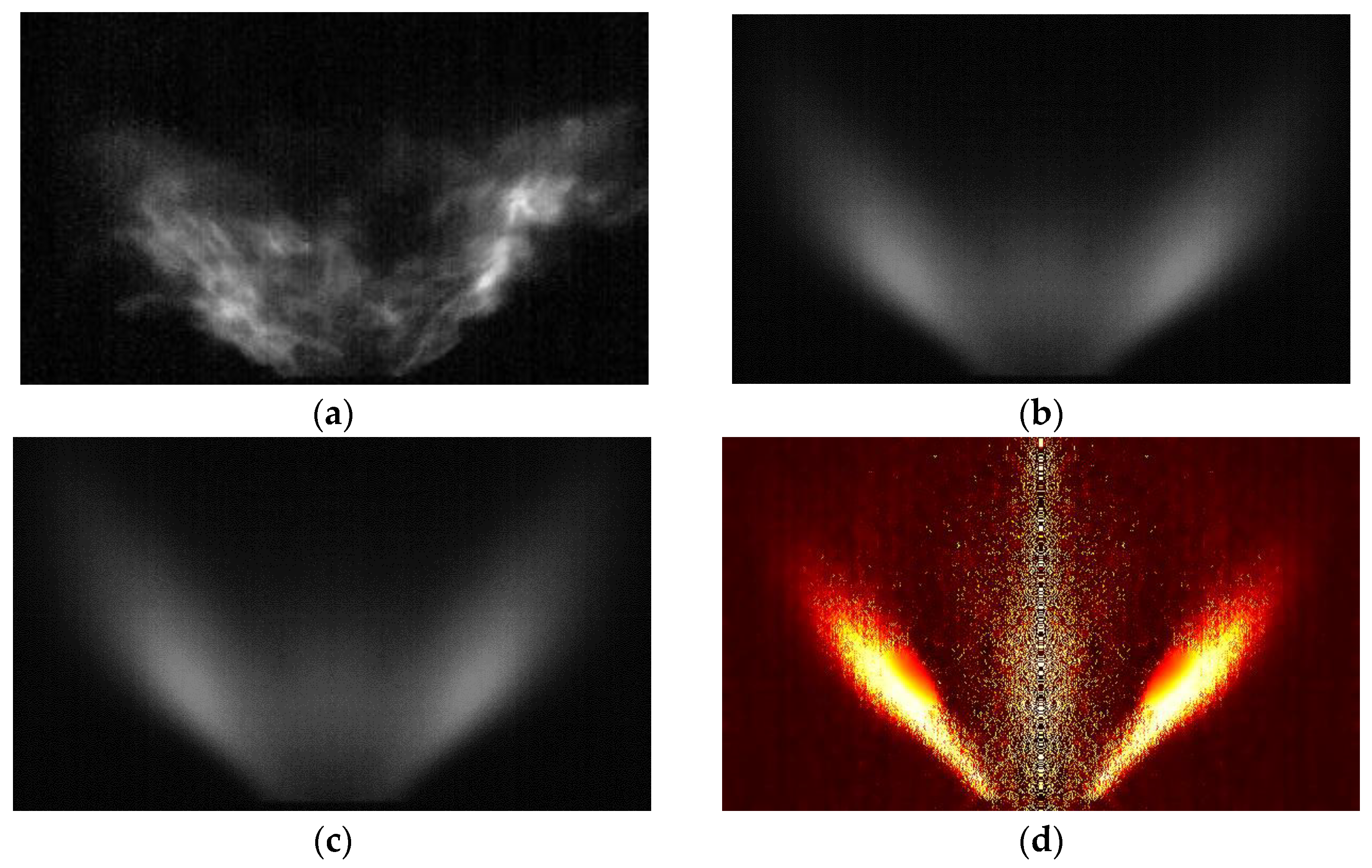
2.3. Flame Image Processing

In order to obtain the unstable combustion characteristics of the flame, the flame images obtained by high-speed CCD are statistically analyzed in this paper, mainly using the inverse Abel transform and POD methods.

2.3.1. Inverse Abel Transform

In this experiment, the flame images under different swirler schemes and working conditions were obtained by using high-speed CCD. Because the high-speed CCD acquires the direct view projection of the combustion area, it is essentially a two-dimensional flame image of line integration in the field of view, which is difficult to reflect the real flame structure. To further analyze the influence of swirler schemes on flame structure, this paper uses inverse Abel transform [30] to process the flame image to reconstruct the flame structure of the central section. The processing is shown in Figure 3. Figure 3a shows the instantaneous image of the flame. It can be seen from the figure that the flame front wrinkles and breaks due to turbulence. Figure 3b shows the time average results of 500 instantaneous images. The characteristic frequencies of unstable combustion obtained in this experiment are all within 350 Hz. Therefore, 500 instantaneous images contain at least one cycle, which can reflect the swept area of the flame front under the unstable combustion state. Figure 3c shows the processing results of the time average image after axisymmetric averaging. Since the inverse Abel transform based on the axisymmetric assumption is adopted, and the actual swirling flow field is affected by the random transport of turbulence, its time average image is not strictly symmetrical, so it is necessary to symmetrically average the time average image along the central axis before the transformation. Finally, inverse Abel transformation is performed on the symmetrical averaged results to obtain the flame structure at the flame center section, as shown in Figure 3d.

2.3.2. POD Method

Proper orthogonal decomposition (POD) is a method that uses orthogonal transformation to extract test variable modes. This paper uses the snapshot POD method based on singular value decomposition (SVD) [31] to process the high-speed flame image in the experiment.

If a flow field parameter sequence at a certain time is expressed as $L_i\in R^{n_p\times 1}$, after extracting the feature information of M snapshots, construct the matrix X, then X can be expressed as:

$$X=\left(L_1,L_2,\dots ,L_{n_t}\right)\in R^{n_p\times n_t}$$

(3)

where p represents the size of the spatial domain, which is much larger than the time t. The inversion matrix $X^T$ is decomposed by SVD, and the process is as follows:

$$[U,S,V]=X^T$$

(4)

where U is an orthogonal matrix and V is an orthogonal eigenvector matrix of $X^T$, that is, POD modal matrix. S is the singular value matrix corresponding to V, that is, $S=diag\left(s_1,s_2,\dots ,s_r\right)$. The elements are sorted according to the energy sequence of the orthogonal basis in the corresponding matrix V, that is, POM, expressed as s_i, then there is s₁ > s₂ > … > s_r. Wherein, the energy proportion of the m_th POD mode is:

$$E^{\left(i\right)}=s_m^2/\sum _{m=1}^M{s}_m^2$$

(5)

3. FTF Optimization Method

3.1. Flame Transfer Function

The flame transfer function (FTF) characterizes the response of the unsteady heat release of the flame to the inlet airflow disturbance, and its mathematical expression is as follows:

$$\mathrm{FTF}(w)=\frac{Q^{\prime }(w)/\overline{Q}}{u^{\prime }(w)/\overline{u}}$$

(6)

where $w$ is the angular frequency, $Q^{\prime }$ and $u^{\prime }$ are the disturbance of heat release rate and velocity, $\overline{Q}$ and $\overline{u}$ are the average. FTF can be obtained by experimental measurement or numerical simulation. During the experimental measurement [32,33,34], it is necessary to add acoustic excitation with different amplitude and frequency at the upstream of the combustor and measure the velocity disturbance at the air inlet and the heat release rate disturbance at the combustor. In the numerical simulation [35,36], it is important to add velocity disturbance near the inlet boundary of the combustor, and monitor the response of the combustor heat release rate disturbance. The above two methods need a lot of repetitive work when obtaining FTF. In order to simplify the modeling process of FTF, based on the experimental data, this paper uses the optimization method to obtain the flame transfer functions under different swirler structures. The specific method is described in Section 3.3.

3.2. Low Order Thermoacoustic Network Model

The low order thermoacoustic network model (LOTAN) can quickly analyze the thermoacoustic stability of the combustion system. In the calculation, LOTAN only considers the one-dimensional plane sound wave in the combustion system. Since the sound wave is greater than the flame thickness, LOTAN ignores the spatial distribution of heat release rate and assumes that the flame surface is infinitely thin. When using the LOTAN method to analyze the thermoacoustic stability, it is first necessary to divide the acoustic units according to the acoustic characteristics of the combustion system. For the model combustor experimental system introduced in Section 2, the LOTAN model can be simply divided into three acoustic units: the rectifier pipe, the intake duct and the combustor. Due to the different flow areas between the rectifier pipe and the intake duct, it is necessary to divide them into different acoustic units. Because there is a flame between the intake duct and the combustor, the flow parameters change suddenly at this position, so it is also necessary to divide them into different acoustic units. The thermoacoustic network model of the model swirl combustor experimental system is shown in Figure 4.

The sound wave is expressed in the form of a Riemann invariant (f and g represent the characteristic amplitude of the incident wave and the reflected wave, respectively), and the upstream and downstream characteristic waves of each acoustic unit are connected by the transfer matrix T:

$$\left(\begin{array}{l}{f}_d\hfill \\ g_d\hfill \end{array}\right)=T(\omega )\left(\begin{array}{l}{f}_u\hfill \\ g_u\hfill \end{array}\right)$$

(7)

The output end of the previous acoustic unit is transferred to the input end of the next acoustic unit, and the calculation is terminated at the boundary condition. All transfer matrices are combined into the following equations:

$$\left(\begin{array}{c}\mathrm{Matrix}\\ \mathrm{of}\\ \mathrm{coefficients}S\end{array}\right)\left(\begin{array}{c}{f}_m\\ g_m\\ ⋮\\ g_n\end{array}\right)=\left(\begin{array}{c}0\\ 0\\ ⋮\\ 0\end{array}\right)$$

(8)

The solution satisfying the characteristic equation $Det(S)=0$ is the characteristic mode of the system, $\omega ={\omega }_{\mathrm{real}}+i{\omega }_{\mathrm{imag}}\in ℂ$. Where ${\omega }_{\mathrm{real}}$ divided by 2π is the characteristic frequency of the system, and the growth rate is ${\omega }_{\mathrm{imag}}$. Near the flame surface, the linear Rankine Hugoniot relationship between unburned gas and burned gas is satisfied:

$${\left(\frac{p^{\prime }}{\rho a}\right)}_d=\frac{{(\rho a)}_u}{{(\rho a)}_d}\left[{\left(\frac{p^{\prime }}{\rho a}\right)}_u-\left(\frac{T_d}{T_u}-1\right)u_u^{\prime }M{a}_u\left(1+\frac{{\dot{Q}}^{\prime }/\overline{\dot{Q}}}{u_u^{\prime }/{\overline{u}}_u}\right)\right]$$

(9)

$$u_d^{\prime }=u_u^{\prime }\left[1+\left(\frac{T_d}{T_u}-1\right)\frac{{\dot{Q}}^{\prime }/\overline{Q}}{u_v^{\prime }/{\overline{u}}_u}\right]-{\left(\frac{p^{\prime }}{\rho a}\right)}_u{\mathrm{Ma}}_u\gamma \left(\frac{T_d}{T_u}-1\right)$$

(10)

The source term ${\dot{Q}}^{\prime }/\overline{Q}$ is given through FTF. FTF can be expressed in many forms. The common linear FTF is Crocco’s famous n − τ model [37]. The mathematical expression of the model is as follows:

$$\frac{{\dot{Q}}^{\prime }(t)}{\overline{\dot{Q}}}=n\frac{u^{\prime }(t-\tau )}{\overline{u}}$$

(11)

where, n is the gain, which represents the amplification effect of heat release rate disturbance on velocity disturbance; τ is the lag time, which represents the characteristic time of fuel from injection to gas generation. The model can capture well the response of heat release rate under weak linear disturbance.

3.3. Optimization Method

Because n and τ are related to many factors, including equivalence ratio, fuel type, combustor structure, intake air speed, etc. [38], therefore, it is not easy to derive the value of n and τ through theoretical calculation. In this context, this paper obtains FTF through the optimization method based on experimental data.

The main idea of this optimization method is that LOTAN first generates a series of acoustic transfer matrices according to the division of acoustic units. Then, a series of weak disturbances is imposed on the inlet boundary, and the disturbances are calculated to the outlet according to the transfer matrix. In the calculation results, the modes that meet the inlet and outlet boundary conditions at the same time are found, which are the characteristic modes of the system. For the characteristic mode of the system, if the growth rate is less than 0, it is a stable combustion mode, and the disturbance will gradually dissipate to 0, and it is unlikely that oscillatory combustion will occur in this mode. The mode with growth rate greater than 0 is unstable, and the disturbance will gradually develop to the limit cycle state; The mode with a growth rate of 0 represents that the combustion system is in a fully developed self-excited oscillation state, and the amplitude of pressure fluctuation presents a stable pulsating state. By generating a sample space of n and τ within a certain range, the FTF described by all sample points in the space is brought into LOTAN for calculation. The calculation results find a mode whose characteristic frequency is close to the real oscillation frequency and the growth rate is close to 0. This mode meets the actual self-excited oscillation of the combustion system, and the corresponding FTF is a reasonable flame transfer function.

After building (n, τ) according to the experimental research results of scholars [39,40], the value range of n is 0~6, and the value range of τ is 0~20 ms. Then, using the Quasi-Monte Carlo sampling method, a two-dimensional Sobol sequence is generated in the range of value space to form a set of (n, τ) value taking sample points. In the optimization process, sample points are obtained through Sobol sampling. Theoretically, the more the number of sampling points, the closer the FTF obtained by optimization is to the true value. However, in the actual process, due to the calculation efficiency, the number of sampling points with appropriate scale should be selected. For this reason, we have adopted the number of sampling points of various scales for calculation, and the calculation results are evaluated by the function D:

$$D=\sqrt{{\left(F_0-F_1\right)}^2+{\left(G_1\right)}^2}$$

(12)

where F₀ is the oscillation frequency obtained from the experiment; F₁ and G₁ are the frequency and growth rate in the LOTAN calculation results, respectively; and the closer D is to 0, the closer the optimization result is to the actual mode. Figure 5 shows the number of samples and their impact on D, which can be seen that when the number > 10,000, D is less than 0.3 and remains at a low level. Therefore, considering the accuracy and efficiency of calculation, this paper selects 20,000 as the appropriate sample size.

4. Results and Discussion

During the experiment, the inlet Reynolds number was kept near 10,055 (inlet speed = 3.2 m/s), the combustion state was adjusted by changing the equivalence ratio, the experimental data were recorded after the working condition was stable, and several experiments were conducted with different swirlers to obtain several combustion conditions. In the experimental results, when the heat release rate and pressure of combustor have obvious main frequency, and the amplitude of dynamic pressure fluctuation in the combustor is large (generally greater than 5%), it can be considered that unstable combustion occurs in the system [41]. Figure 6 shows the pressure signal and its spectrum in the combustor under stable combustion and unstable combustion states of swirler B.

Figure 7 shows the combustion state under different swirlers and different equivalence ratios. The square symbol represents the stable combustion state, and the triangle symbol represents the unstable combustion state. It can be seen that, first, with the decrease in equivalence ratios, the combustion state under the three swirler schemes gradually transits from stable combustion to unstable combustion; Second, the self-excited oscillation frequency under each swirler increases with the increase in the equivalence ratios, which is mainly because the increase in the equivalence ratios leads to the increase in the average temperature of the combustor and the increase in the sound velocity; under the same combustor geometry, the wave number increases and the frequency also increases accordingly.

The influence of swirler schemes on combustion is mainly shown in two aspects: first, the structure of the swirler affects the boundary of combustion stability, and the critical equivalence ratios for unstable combustion are different under different swirler schemes; Second, the oscillation frequency when unstable combustion occurs under different swirl intensities is also different. The characteristic frequency when unstable combustion occurs in swirler A is approximately 319 Hz, the characteristic frequency when unstable combustion occurs in swirler B is approximately 280 Hz, and the characteristic frequency of swirler C is approximately 290 Hz. The characteristic frequency does not change monotonously with the swirl intensity (the swirl intensity of A is the strongest, followed by B, and C is the weakest). Under the action of the swirling flow of different intensity, the pulsation structure of the flame is different, and the unsteady heat release in the combustion zone is also different, so the flame transfer function of the combustor is also different. Different swirlers affect the characteristic frequency of unstable combustion of the combustion system by affecting the lag time term in the FTF. The influence of swirler schemes on combustion instability will be detailed in Section 4.2.

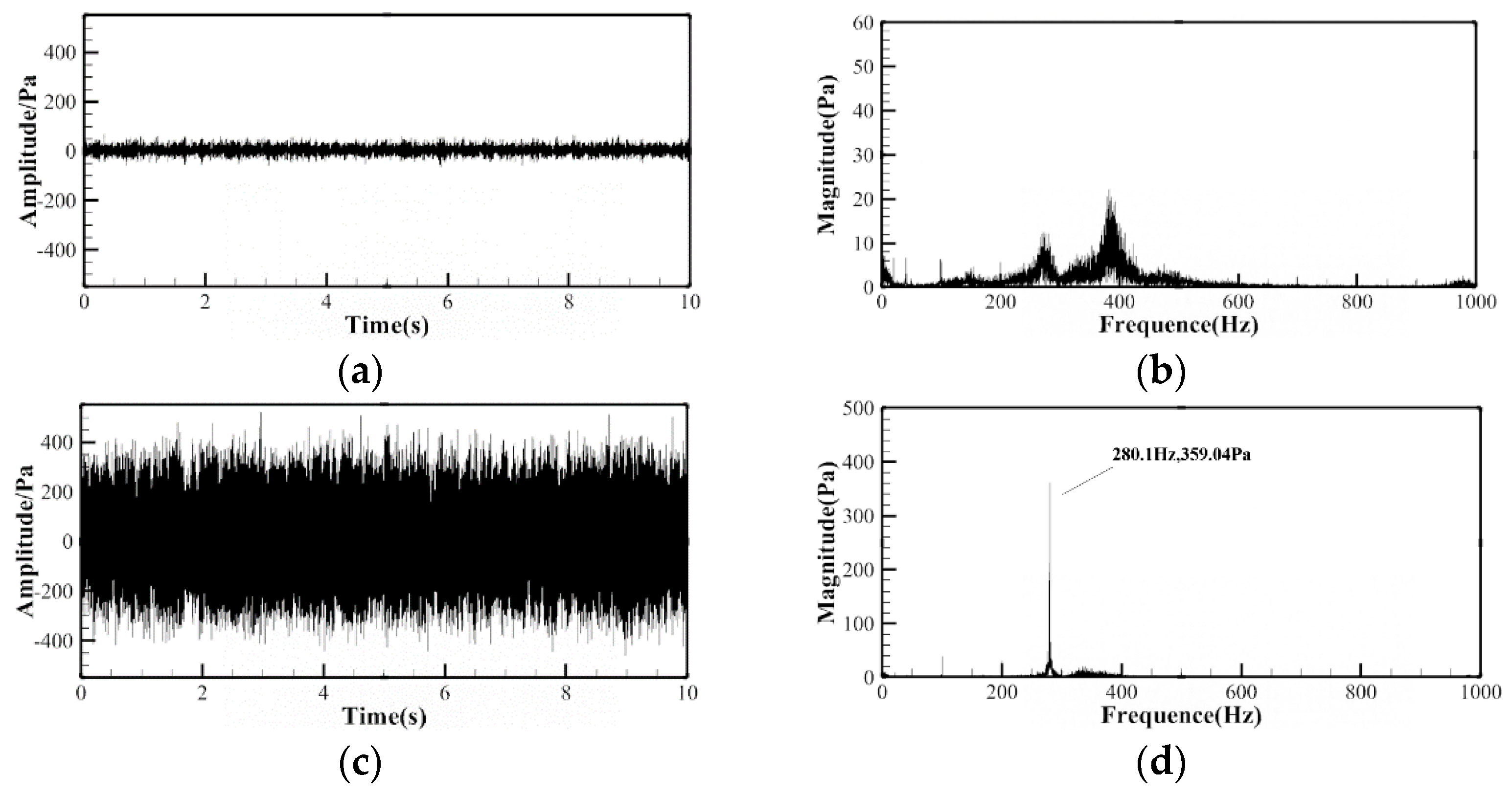
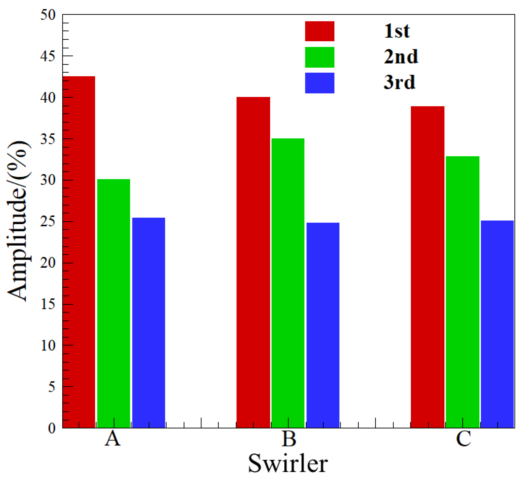
4.1. Influence of Swirler on Flame Pulsation Characteristics

The pulse structure in the process of flame oscillation can be obtained by POD of high-speed flame images. After counting the energy proportions of each order under different working conditions, it is found that the total energy proportion of the first three orders is more than 95%, indicating that the flame pulsation is mainly concentrated in the first three orders of POM. Figure 8 shows the decomposition results of the first three POD modes in the unstable combustion state under three groups of swirlers. The yellow and blue represent the peaks and troughs of the pulsating amplitude, respectively, and the adjacent peaks and troughs represent the pulsating structure of the flame in space.

Swirler A and swirler C have similar pulsating characteristics of heat release rate. When unstable combustion occurs, there are obvious longitudinal pulsating structures in the first and second modes, indicating that the flame in the combustor will be continuously stretched and flashed back; Swirler B is in a medium intensity swirling state, and the areas with the strongest fluctuations in the first and second modes are mainly located in the shear layer near the root of the swirler. In the three groups of swirlers, the third-order mode pulsation area is similar, all concentrated at the root of the flame, and the third-order mode is relatively close to the rotating mode of the flame.

Figure 9 shows the proportions of the singular value total energy of the first three modes of the three swirlers in the case of unstable combustion. With the decrease in swirl number, the energy proportion of the first order singular value decreases gradually. For the energy proportion of the second order singular value, swirler B is the highest, swirler C is the second, and swirler A is the lowest; The energy proportion of the third order singular value between different swirlers has little difference. This shows that the first two order pulsating modes are mainly affected by different swirlers.

4.2. Influence of Swirler on FTF

The experimental results show that the influence of swirler scheme on the characteristics of unstable combustion is relatively complex, and the characteristic frequency of unstable combustion in the combustor does not change monotonously with swirl intensity. In order to further explore the cause of this phenomenon, this paper analyzes it in combination with the flame transfer function (FTF). The change in swirler structure will affect the downstream flow field, which will be further reflected in the unsteady heat release characteristics of the flame. Based on the experimental data, this paper uses the optimization method to obtain the FTF under the same working condition (air inlet speed is 3.2 m/s, equivalence ratio is 0.21) and different swirler structures so as to reflect the response characteristics of heat release rate. The optimization results are shown in

Table 2. FTF under different swirler structures.

Swirler	n	τ/ms
A	4.702	6.230
B	4.710	7.138
C	4.949	6.846

. Figure 10 shows the modal distribution of three groups of swirlers under the optimized FTF calculated based on the LOTAN model. The position with the deepest color (represented by the pentagram) is the characteristic mode of the system, and the black dotted line is the oscillation frequency measured in the experiment. It can be seen that each swirler has established a limit cycle state near the oscillation frequency. For swirlers A and B, within the “dangerous” frequency range of 250–350 Hz (under all operating conditions, the oscillation frequency of the model combustor is within this range), there are two modes in the system, but the growth rate of characteristic modes outside the oscillation frequency is far from 0, indicating that the system still has the trend of continuous development.

According to the calculation results in Table 2, under the same working conditions, the gain n of the three swirlers has little difference. This is because the gain n represents the amplification effect of the heat release rate disturbance on the inlet disturbance of the combustion zone. Under the same inlet conditions and equivalence ratio, the overall heat release rate of the combustor is approximately the same, so the gain n is basically the same. Figure 11 shows the comparison of CH* signals of the three swirlers when the equivalence ratio is 0.21. It can be seen that under the same working conditions, the disturbance level of heat release rate in the combustor of the three groups of swirlers has little difference.

For the lag time τ, the optimization results show that the lag time of swirler A is the shortest, followed by that of swirler C, and the lag time of swirler B is the longest. Lag time represents the characteristic time that the fuel experiences from the nozzle to the complete gas. In this process, the fuel micro cluster mainly undergoes several sub processes, such as mixing, convection and chemical reaction. According to the research results of Kim et al. [42], for gaseous fuels, the convective transport process accounts for the largest proportion in the lag time, usually more than 93%, and the convection time can be calculated by the following equation [40,43]:

$${\tau }_{\mathrm{conv}}=l/u_{\mathrm{conv}}$$

(13)

where l is the flame length, and u_conv is the average axial velocity of fuel flow at the swirler outlet. Figure 12 shows the flame structures under different swirlers obtained by Abel inverse transformation and their axial (normalization) light intensity signal distribution. It is defined that the axial distance between the positions of the dimensionless light intensity signal 0.4 at the head and 0.4 at the tail of the flame is the flame length L_f. It can be seen that when the swirl intensity is high, the flame length is short, while when the swirl intensity is low, the flame length is long. When the swirl intensity is high, the tangential velocity increases, the recirculation zone becomes shorter, and the flame distribution becomes shorter. On the other hand, with the increase in the tangential velocity, the shear strength of the central recirculation zone and the corner recirculation zone increases, which promotes the mixing process of fuel and air and shortens the length of the diffusion flame.

According to the corresponding relationship between the pixel and the actual physical distance (1 px = 0.28 mm), the flame length L_f under A, B and C swirlers is 68.175 mm, 83.611 mm and 85.12 mm, respectively.

Due to the complex flow field structure of the two-stage swirl combustor, it is difficult to measure the axial velocity at the outlet of the swirler through experiments. The velocity field of the swirl flow is obtained using RANS with commercial CFD software Fluent 19.0. In this study, the realizable k-ε model is used for the turbulence model, which was fully proved and verified in a turbulent swirling gas turbine combustor [44,45]. The eddy dissipation (ED) model is used as the combustion model. Previous RANS studies using the ED model show that the calculation results of the ED model are in good agreement with the experimental results in capturing swirling flame structure [44]. The commercial software UG NX10.0 was used to build the three-dimensional model of the combustor in 1:1 scale. Unstructured mesh is generated for complex combustor head. Structured mesh is generated for the combustion chamber. After grid independence tests, the total number of cells is approximately 7.3 million. The Figure 13 shows the CFD calculation domain (generated using ANSYS ICEM 19.0).

Then, the average axial velocity of fuel at the outlet of swirler, u_conv, is obtained by RANS calculation. The amount of calculation grid is approximately 7.8 million, the calculation condition is consistent with the test condition, and the turbulence model is the realized k-e model. Figure 14 shows the axial velocity contour of the combustor under swirler A, in which the structure of the shear layer and the central recirculation zone can be clearly seen, and it can be seen that the axial velocity at the outlet of the two stages of the swirler is different.

Figure 15 shows the axial velocity distribution near the outlet of three swirlers (i.e., the dotted line position in the Figure 14). It can be seen that there are two peaks in the figure, corresponding to the outlet positions of two stages of swirlers. For swirler A, the axial velocity at the outlet of the internal primary swirler is approximately 14.5 m/s, and the axial velocity at the outlet of the external secondary swirler is approximately 8.3 m/s. The average axial velocity near the swirler outlet, u_conv, is 11.4 m/s. The lag time calculated by Equation (13) is approximately 5.98 ms, which is slightly less than the calculated lag time (6.23 ms). This is because the lag time is a global quantity. The current processing takes the airflow velocity at the outlet of the swirler as the global average velocity. However, in fact, this ignores the loss when the velocity flows along the axis, so the calculation result is smaller than the actual result.

Similarly, the average axial velocity distribution at the outlet of swirler B and swirler C is obtained, and the average axial velocity at the outlet of the two stages of swirlers is 12.25 m/s and 13.73 m/s, respectively. According to Formula (12), the lag time under swirler B and swirler C is 6.82 ms and 6.20 ms, respectively. Figure 16 shows the comparison between the optimized lag time and the lag time obtained by Formula (12). It can be seen that the results are relatively close, and the trend is basically consistent, indicating that the optimization method is reasonable, and the FTF obtained by optimization is relatively accurate.

From the above analysis, it can be concluded that the change in lag time with swirl intensity is not monotonous, because with the increase in swirl intensity, the flame length will shorten, but the axial velocity of the fuel outlet will also decrease, and the change rate of both will affect the change direction of lag time. Figure 17 shows the influence of the lag time on the thermoacoustic system oscillation mode. The purple area in the figure is the unstable area. When the lag time is τ in this area, the phase relationship between the heat release rate and the pressure meets the Rayleigh criterion [46], which will cause coupling oscillation and an unstable combustion system. It can be seen from the figure that when the system lag time is short, the system is more likely to oscillate in the high-frequency mode, as shown in the curve below Figure 17; When the lag time of the system is longer, the system is more likely to oscillate in the lower frequency mode. In the three swirler experiments conducted in this paper, the lag time of swirler B is the longest, so the oscillation frequency is the lowest.

5. Conclusions

In this paper, the unsteady combustion characteristics of the model combustor under different swirl intensities are studied by experiment and simulation, and the flame transfer function (FTF) under different swirler schemes is obtained by the optimization method. The experimental results show that the stable combustion equivalence ratio boundary of the combustor decreases with the decrease in swirl intensity. However, the oscillating combustion frequency of the combustor does not simply change monotonously with the change in swirl intensity. For swirler A with the largest swirl intensity, the oscillating frequency is approximately 319 Hz; for swirler B with medium swirl intensity, the oscillating frequency is approximately 280 Hz; and for swirler C with the smallest swirl intensity, the oscillating frequency is approximately 290 Hz. According to the analysis results of the combustor’s flame transfer function, the gain term n is mainly controlled by the heat release in the combustor. Therefore, under the same working conditions, the gain term n of three swirlers are basically the same, and swirler A, B and C are 4.702, 4.710 and 4.949, respectively. Swirl intensity mainly affects the lag time term τ of the combustion system and then affects the oscillating combustion frequency. The lag time is mainly affected by two factors: one is the flame length, the other is the convection time. The increase in swirl intensity will shorten the flame length, but at the same time, it will also reduce the axial convection velocity. The change rate of the two determines the change direction of the lag time. For the lag time, the results of optimization and experiment combined with simulation reflect the same trend. The lag time of three swirlers are 5.98 ms, 6.82 ms and 6.20 ms, respectively.

Based on the above research conclusions, in the design stage, designers need to consider not only the flame stability performance of swirler but also the influence of the swirl intensity on the characteristic frequency of unstable combustion to avoid coupling the thermoacoustic oscillation mode with the inherent acoustic mode of the system, which will cause damage to the combustor structure. However, the effect of swirl intensity on the characteristic frequency of the combustion chamber is not a simple monotonous relationship, which needs to be considered in combination with the flame structure and convection velocity. In addition, this research also proposes a flame transfer function optimization method with engineering application value. Compared with the traditional method using acoustic excitation, this method can quickly optimize the FTF under different working conditions based on experimental data, with higher calculation efficiency, and the calculation results also correspond well to the experimental and simulation results, which have practical physical significance.

The existing research work only discusses the phenomenon captured in the experimental process (the characteristic frequency does not change monotonously with the swirl intensity) from the perspective of FTF analysis, which can explain this physical phenomenon from the lag time. However, this part of the work cannot provide enough guidance for the swirler designer. In the future, our team will continue to deeply study the physical driving mechanism behind the unstable combustion of the swirling flame in combination with the flame dynamics and consider the impact of more swirler structure parameters (such as the number of blades, the size of the swirler, etc.) on the thermoacoustic stability of the combustor, so as to provide more reference for the designer.

References

1. Zhang, C.Y. The Mechanism and Control for Combustion Instabilities of Aeroengine Afterburner. Ph.D. Thesis, Beihang University, Beijing, China, 2010. (In Chinese). [Google Scholar]
2. Huang, L. Investigation on the Mechanism of Combustion Oscillation in a LPP Combustor. Master’s Thesis, Nanjing University of Aeronautics, Nanjing, China, 2016. (In Chinese). [Google Scholar]
3. Orth, M.R.; Vodney, C.; Liu, T.; Hallum, W.Z.; Pourpoint, T.L.; Anderson, W.E. Measurement of linear growth of self-excited instabilities in an idealized rocket combustor. In Proceedings of the 2018 AIAA Aerospace Sciences Meeting, Kissimmee, FL, USA, 8–12 January 2018. [Google Scholar]
4. Poinsot, T. Prediction and control of combustion instabilities in real engines. Proc. Combust. Inst. 2017, 36, 1–28. [Google Scholar] [CrossRef] [Green Version]
5. Sarli, V.D.; Marra, F.S.; Benedetto, A.D. Spontaneous oscillations in lean premixed combustors: CFD simulation. Combust. Sci. Technol. 2007, 179, 2335–2359. [Google Scholar] [CrossRef]
6. Di Sarli, V.; Di Benedetto, A.; Marra, F.S. Influence of system parameters on the dynamic behaviour of an LPM combustor: Bifurcation analysis through CFD simulations. Combust. Theory Model. 2008, 12, 1109–1124. [Google Scholar] [CrossRef]
7. Garcia-Agreda, A.; Di Sarli, V.; Di Benedetto, A. Bifurcation analysis of the effect of hydrogen addition on the dynamic behavior of lean premixed pre-vaporized ethanol combustion. Int. J. Hydrogen Energy 2012, 37, 6922–6932. [Google Scholar] [CrossRef]
8. Kojourimanesh, M.; Kornilov, V.; Arteaga, I.L.; de Goey, L.P.H. Theoretical and experimental investigation on the linear growth rate of the thermo-acoustic combustion instability. In Proceedings of the 10th European Combustion Meeting, Naples, Italy, 14–15 April 2021. [Google Scholar]
9. Durox, D.; Schuller, T.; Gandel, S. Self-induced instability of a premixed jet flame impinging on a plate. Proc. Combust. Inst. 2002, 29, 69–75. [Google Scholar] [CrossRef]
10. Yang, Y.; Yu, Z.J. Stability analysis of swirl premixed flame based on flame transfer function. Gas Turbine Technol. 2021, 34, 14–20. (In Chinese) [Google Scholar]
11. Sun, X.F. Study on Dynamics of Partially Premixed Flames by Large Eddy Simulation Combined with System Identification. Master’s Thesis, University of Chinese Academy of Sciences, Beijing, China, 2019. (In Chinese). [Google Scholar]
12. Kraus, C.; Selle, L.; Poinsot, T. Coupling heat transfer and large eddy simulation for combustion instability prediction in a swirl burner. Combust. Flame 2018, 191, 239–251. [Google Scholar] [CrossRef] [Green Version]
13. Meloni, R.; Ceccherini, G.; Michelassi, V. Analysis of the self-excited dynamics of a heavy-duty annular combustor by large-eddy simulation. J. Eng. Gas Turbines Power 2019, 141, 111016. [Google Scholar] [CrossRef]
14. Silva, C.F.; Emmert, T.; Jaensch, S. Numerical study on intrinsic thermoacoustic instability of a laminar premixed flame. Combust. Flame 2015, 162, 3370–3378. [Google Scholar] [CrossRef]
15. Kaiser, T.L.; Öztarlik, G.; Selle, L. Impact of symmetry breaking on the Flame Transfer Function of a laminar premixed flame. Proc. Combust. Inst. 2019, 37, 1953–1960. [Google Scholar] [CrossRef] [Green Version]
16. Nicoud, F.; Benoit, L.; Sensiau, C. Acoustic modes in combustors with complex impedances and multidimensional active flames. AIAA J. 2007, 45, 426–441. [Google Scholar] [CrossRef]
17. Ni, F.; Nicoud, F.; Méry, Y. Including flow–acoustic interactions in the Helmholtz computations of industrial combustors. AIAA J. 2018, 56, 4815–4829. [Google Scholar] [CrossRef]
18. Stow, S.R.; Dowling, A.P. Thermoacoustic oscillations in an annular combustor. In Proceedings of the ASME TURBO EXPO, New Orleans, LA, USA, 4–7 June 2001. [Google Scholar]
19. D’Alessandro, S.; Frezzotti, M.L.; Favini, B. A Multi-dimensional Approach for Low Order Modeling of Combustion Instability in a Rocket Combustor. In Proceedings of the Joint Propulsion Conference, Cincinnati, OH, USA, 9–11 July 2018. [Google Scholar]
20. Yang, F.J.; Guo, Z.H.; Fu, X. Combustion Instability Analysis Based on Thermoacoustic Network Method. J. Propuls. Technol. 2014, 35, 822–829. (In Chinese) [Google Scholar]
21. Weng, F.L.; Zhou, S.W.; Zhu, M. Modeling and Simulation of combustion oscillation based on description function. J. Propuls. Technol. 2021, 42, 2306–2314. (In Chinese) [Google Scholar]
22. He, Z.Q.; Wang, P.; Meenatchidevi, M. Experimental study on thermoacoustic oscillation in a new Double Swirl Combustor. J. Exp. Fluid Mech. 2021, 35, 44–52. (In Chinese) [Google Scholar]
23. Kim, K.T. Combustion instability feedback mechanisms in a lean-premixed swirl-stabilized combustor. Combust. Flame 2016, 171, 137–151. [Google Scholar] [CrossRef]
24. Choi, J.J.; Rusak, Z.; Kapila, A.K. Numerical simulation of premixed chemical reactions with swirl. Combust. Theory Model. 2007, 11, 863–887. [Google Scholar] [CrossRef]
25. Wang, S.; Hsieh, S.Y.; Yang, V. Unsteady flow evolution in swirl injector with radial entry: I. Stationary conditions. Phys. Fluids 2005, 17, 045106. [Google Scholar] [CrossRef] [Green Version]
26. Ateshkadi, A.; McDonell, V.G.; Samuelsen, G.S. Effect of hardware geometry on gas and drop behavior in a radial mixer spray. Symp. (Int.) Combust. 1998, 27, 1985–1992. [Google Scholar] [CrossRef]
27. Palies, P.; Durox, D.; Schuller, T. The combined dynamics of swirler and turbulent premixed swirling flames. Combust. Flame 2010, 157, 1698–1717. [Google Scholar] [CrossRef]
28. Huang, Y.; Yang, V. Dynamics and stability of lean-premixed swirl-stabilized combustion. Prog. Energy Combust. Sci. 2009, 35, 293–364. [Google Scholar] [CrossRef]
29. Nori, V.N.; Seitzman, J.M. CH∗ chemiluminescence modeling for combustion diagnostics. Proc. Combust. Inst. 2009, 32, 895–903. [Google Scholar] [CrossRef]
30. Keefer, D.R.; Smith, L.M.; Sudharsanan, S.I. Abel inversion using transform techniques. J. Quant. Spectrosc. Radiat. Transf. 1988, 39, 367–373. [Google Scholar]
31. Lai, A.Q.; Liu, Y.P.; Fu, Y.M. Image processing of combustion oscillation flame. J. Combust. Sci. Technol. 2020, 26, 8. (In Chinese) [Google Scholar]
32. Zhu, R.; Pan, D.; Ji, C. Combustion instability analysis on a partially premixed swirl combustor by thermoacoustic experiments and modeling. Energy 2020, 211, 118884. [Google Scholar] [CrossRef]
33. Palies, P.; Durox, D.; Schuller, T. Nonlinear combustion instability analysis based on the flame describing function applied to turbulent premixed swirling flames. Combust. Flame 2011, 158, 1980–1991. [Google Scholar] [CrossRef]
34. Yu, D.; Guo, Z.H.; Yang, F.J. Analysis of distributed flame transfer function in lean premixed combustor. J. Propuls. Technol. 2016, 37, 2210–2218. (In Chinese) [Google Scholar]
35. Merk, M.; Jaensch, S.; Silva, C. Simultaneous identification of transfer functions and combustion noise of a turbulent flame. J. Sound Vib. 2018, 422, 432–452. [Google Scholar] [CrossRef]
36. Han, X.; Morgans, A.S. Simulation of the flame describing function of a turbulent premixed flame using an open-source LES solver. Combust. Flame 2015, 162, 1778–1792. [Google Scholar] [CrossRef] [Green Version]
37. Crocco, L. Aspects of combustion stability in liquid propellant rocket motors part I—Fundamentals: Low frequency instability with monopropellants. J. Am. Rocket. Soc. 1951, 21, 163–178. [Google Scholar] [CrossRef]
38. Harrje, D.T.; Reardon, F.H. Liquid Propellant Rocket Combustion Instability; Scientific and Technical Information Office, National Aeronautics and Space Administration: Oak Ridge, TN, USA, 1972.
39. Hield, P.A.; Brear, M.J.; Jin, S.H. Thermoacoustic limit cycles in a premixed laboratory combustor with open and choked exits. Combust. Flame 2009, 156, 1683–1697. [Google Scholar] [CrossRef]
40. Bernier, D.; Lacas, F.; Candel, S. Instability mechanisms in a premixed prevaporized combustor. J. Propuls. Power 2004, 20, 648–656. [Google Scholar] [CrossRef]
41. Sun, P.F.; Ge, B.; Yuan, Y.R.; Zang, S.S. Oscillation combustion mechanism of LPP combustor and suppression of oscillation by secondary fuel. J. Eng. Therm. Energy Power 2018, 33, 36–42. (In Chinese) [Google Scholar]
42. Kim, D.; Joo, S.; Yoon, Y. Effects of fuel line acoustics on the self-excited combustion instability mode transition with hydrogen-enriched laboratory-scale partially premixed combustor. Int. J. Hydrogen Energy 2020, 45, 19956–19964. [Google Scholar] [CrossRef]
43. Yoon, J.; Joo, S.; Kim, J. Effects of convection time on the high harmonic combustion instability in a partially premixed combustor. Proc. Combust. Inst. 2017, 36, 3753–3761. [Google Scholar] [CrossRef]
44. Anisimov, V.; Chiarioni, A.; Rofi, C.; Ozzano, S.; Hermeth, G.; Hannebique, G.; Staffelbach, G.; Poinsot, T. Bi-stable flame behavior of heavy duty gas turbine burner, RANS, LES and experiment comparison. In Proceedings of the ASME Turbo Expo 2015: Turbine Technical Conference and Exposition, Montreal, QC, Canada, 15–19 June 2015. Paper No. GT2015-42536. [Google Scholar]
45. Rofi, L.; Campa, G.; Anisimov, V.; Dacca, F.; Bertolotto, E.; Gottardo, E.; Bonazni, F. Numerical procedure for the investigation of combustion dynamics in industrial gas turbines: LES, RANS and thermoacoustics. In Proceedings of the ASME Turbo Expo 2015: Turbine Technical Conference and Exposition, Montreal, QC, Canada, 15–19 June 2015. Paper No. GT2015-42168. [Google Scholar]
46. Rayleigh, J.S.W. The Theory of Sound; Dover Publications: New York, NY, USA, 1945. [Google Scholar]
Figure 1. Structure sketch of swirler. (a) Swirler structure; (b) Geometry of the injection unit; (c) Swirler parameters.
Energies 15 08972 g001
Figure 2. Schematic diagram of model combustor experimental setup.
Energies 15 08972 g002
Figure 3. Reconstruction process of flame center section. (a) Instantaneous image; (b) Time average image; (c) Symmetrical average; (d) Inverse Abel transform.
Energies 15 08972 g003
Figure 4. LOTAN of model combustor experimental system.
Energies 15 08972 g004
Figure 5. Influence of sample number on accuracy.
Energies 15 08972 g005
Figure 6. DP time-series signal and frequency spectra of steady and unstable combustion. (a,b) Stable combustion state, equivalence ratio is 0.285; (c,d) Unstable combustion state, equivalent ratio is 0.228.
Energies 15 08972 g006
Figure 7. Influence of swirler scheme and equivalence ratio on combustion state.
Energies 15 08972 g007
Figure 8. POD results under different swirlers. (ac) The first three modes of swirler A; (df) swirler B; (gi) swirler C.
Energies 15 08972 g008
Figure 9. The first three order singular value energy proportions of different swirlers.
Energies 15 08972 g009
Figure 10. Modal distribution of three swirler schemes under optimized FTF. (a) Swirler A; (b) Swirler B; (c) Swirler C. (The pentagram represents the characteristic mode, and the dotted line is the characteristic frequency measured in the test).
Energies 15 08972 g010
Figure 11. CH* signal in combustor under different swirler schemes (a,b).
Energies 15 08972 g011
Figure 12. Flame structure and axial light intensity distribution under different swirler structures. (a)swirler A; (b) swirler B; (c) swirler C.
Energies 15 08972 g012
Figure 13. Computational mesh for CFD model.
Energies 15 08972 g013
Figure 14. Contour of axial velocity of combustor under swirler A. (unit: m/s).
Energies 15 08972 g014
Figure 15. Average axial velocity at the outlet of swirlers.
Energies 15 08972 g015
Figure 16. Comparison of LOTAN optimization with lag time obtained by formula calculation.
Energies 15 08972 g016
Figure 17. Schematic diagram of the influence of lag time on oscillation mode.
Energies 15 08972 g017