Improved Thermal Performance of a Serpentine Cooling Channel by Topology Optimization Infilled with Triply Periodic Minimal Surfaces

Abstract

The present study utilizes a density-based topology optimization method to design a serpentine channel under turbulent flow, solving a high pressure loss issue and enhancing heat transfer capability. In the topology optimization, the k–ε turbulence model is modified by adding penalization terms to reveal turbulence effects. Heat transfer modeling is included by setting the modified energy equation with additional terms related to topology optimization. The main objective is to minimize pressure loss while restricting heat transfer. The 2D simplified model is topologically optimized. Then, the optimal solution with intermediate results is extruded in the 3D system and interpreted with triply periodic minimal surfaces (TPMS) to further enhance heat transfer performance. Compared to the baseline serpentine channel, the optimized model infilled with the diamond-TPMS structure lowers pressure loss by 30.8% and significantly enhances total heat transfer by up to 45.8%, yielding thermal performance of 64.8% superior to the baseline. The temperature uniformity is also improved. The simulation results show that the curvatures in the optimized model with diamond-TPMS structure eliminate the large recirculation flow and low heat transfer regions. This model diminishes the effect of Dean’s vortices but promotes high turbulent kinetic energy, leading to better uniform flow and heat transfer distributions.

1. Introduction

Applications of a multipass cooling channel under turbulent flow and heat transfer enhancement themes can be found in an internal cooling gas turbine blade, microelectronic cooling, etc. Generally, the serpentine channel is a standard internal cooling scheme in practical turbine blades, effectively utilizing the coolant in the midchord region [1,2]. However, complicated flow fields induced by sharp turns after bend regions cause a nonuniform flow distribution. Rao et al. [3] have reported that the turning regions cause more than 90% of the total pressure drop of the multipass channel. These phenomena in the serpentine channels result in highly nonuniform-flow heat transfer and high pressure loss, decreasing overall thermal performance. Therefore, it is desirable to design multipass channels that generate a lower-pressure loss while maintaining the total heat transfer and achieving better uniformity.

In order to control the flow field and heat transfer distribution in serpentine channels, placing the turning guide vane at the bend region is a common method that has been examined in several previous studies. Schüler et al. [4] and Guo et al. [5] investigated experimentally and numerically different turning guide vane designs in the multipass channel. They found that the pressure loss was reduced by about 13.4%–48.4% when using the turning guide vanes, but the heat transfer deteriorated. Similarly, Lei et al. [6] observed that the pressure loss was largely reduced when installing the turning vane, yet heat transfer decreased because the flow separation was suppressed. This design process was based on a trial-and-error method. To achieve low pressure loss while maintaining total heat transfer in a serpentine cooling channel, various geometrical parameters were varied, causing a cost- and time-consuming design process.

Alternatively, optimization methods can speed up and ease the designs. Layout optimization is usually divided into size, shape and topology optimization (TO). Size and shape optimizations have been used to minimize pressure loss and enhance thermal performance in heat exchangers. The results reveal that the optimal design significantly reduces the pressure drop and achieves higher thermal efficiency than the original model [7]. However, it is observed that the design process only adjusts the positions of points or boundaries of the channel to obtain the objective functions without changing the topology of the structure. Moreover, since additive manufacturing is rapidly developed, which can compete for limitations to produce relatively complex geometries, the size and shape optimizations cannot completely exploit this manufacturing scheme’s potential. Meanwhile, finding the optimal shapes and optimizing the topology of channels can be obtained simultaneously through topology optimization. Additionally, free-form and efficient geometries can be generated, satisfying solutions for additive manufacturing. Therefore, topology optimization is a more general design method than size and shape optimizations [8].

Topology optimization has been employed in different design systems covered by various disciplines. It has been well developed and affirmed widely due to competitive designs in cost and functionality under various constraints [8,9,10,11,12,13,14]. Several methods, such as the homogenization approach, the evolutionary technique, the level-set and the density approach, have been developed for implementation.

Among topology optimization schemes, the density-based method has gained more popularity [15]. In the comparisons of Manuel et al. [16], the density-based approach yields better outcomes for most cases in terms of iteration numbers. Additionally, the density method merits rapid convergence and weak dependence on the initial guess [8,16]. Furthermore, it could be highlighted that no prior research has considered turbulent flow systems except the density-based method. The key idea of the density-based method is the penalized interpolation function, which continuously forces fictitious porous cells, including fluid and solid, to be fluid or solid subdomains. A comprehensive review and its general formulation of topology optimization can be found in previous work [8]. Here, a brief overview of the density-based topology optimization applied in recent research on thermofluid systems is shown in

Table 1. An overview of density-based topology optimization in recent studies on thermofluid systems.

Author	Flow Regime	Structure	Discretization	Optimizer
Alexandersen et al. [17]	Laminar	2D and 3D	FEM 1	MMA 3
Dilgen et al. [18]	Turbulent	2D and 3D	FVM 2	MMA
Haertel et al. [19]	Laminar	2D	FEM	GCMMA 4
Li et al. [20,21]	Laminar	2D	FEM	SNOPT 5
Zhang et al. [22]	Laminar	2D	FEM	GCMMA

¹ finite element method. ² finite volume method. ³ method of moving asymptotes. ⁴ globally convergent method of moving asymptotes. ⁵ sparse nonlinear optimizer.

.

As highlighted in Table 1, most previous studies are 2D models with a steady-state laminar flow regime. The FEM is the most implemented discretization method since the topology optimization initiates from solid mechanics. Moreover, it is easier for the discrete adjoint scheme to manage the FEM [15].

Nevertheless, only limited works on turbulent flow topology optimization have been studied, which is primarily needed in most industrial flow applications, e.g., a turboshaft engine’s turbine blade serpentine cooling channels. Several works employed a frozen turbulence assumption to simplify sensitivity analysis for the topology optimization of turbulent flows [23,24]. However, as the frozen turbulence neglects the effect of porosity in the turbulent viscosity calculation, the optimized model negatively affects the accuracy. The shortcomings of this assumption have been presented by Dilgen et al. [25].

Recently, study of the turbulence effects in the topology optimization for turbulent flow has appeared. Dilgen et al. [25] optimized many 2D and 3D complex flow channels using Spalart–Allmaras and k–ω turbulence models, where k denotes turbulent kinetic energy and ω is the specific dissipation rate. The results showed that the generated structure in a U-bend channel significantly reduced the pressure drop across the channel. Later, Yoon [26] proposed the topology optimization with the FEM using the k–ε turbulence model, where ε is the turbulent energy dissipation. However, it is noted that the energy equation for topology optimization has not yet been found, and convective heat transfer optimization has not yet been explored in those studies.

Even though topology optimization is an efficient tool for generating complex structures, it still causes some problems. The results of density-based topology optimization may convert a number of intermediate densities. This type of conversion causes pressure maldistribution in the cooling channel between the design and its realization by additive manufacturing, which could not explore the full performance of the optimized structure. To overcome the issues, the solid domain of the optimized model, including the intermediate results, can be fulfilled with a graded lattice structure. This method has been observed to help manage the intermediate densities in the conventional topology optimization, reduce the structure’s weight, and preserve the original design structure [27]; however, this approach is rarely applied to cooling channel applications.

Among complex lattice structures, the repeating network, called triply periodic minimal surface (TPMS), has attracted much research interest due to its compact and significant thermal properties. Additionally, the TPMS is a self-supporting structure, which has been observed to present better mechanical performance than other strut-based lattice structures [28]. The TPMS networks have also shown better heat transfer performance in cooling channels than the lattice-frame material due to a smoother surface and larger wetted area [29]. The TPMS, with its complex and interconnected structures, provided consistent fluid streamlines, promoting permeation [30]. Moreover, many previous works have found that the TPMS structures considerably increase heat transfer with reasonably increased pressure loss, improving the thermal performance of the cooling channel [31,32,33].

This work proposes an optimized design to minimize pressure and increase heat transfer, improving the thermal performance of a serpentine cooling channel. The density-based topology optimization for the thermofluid problem under turbulent flow is firstly utilized to minimize the pressure loss while maintaining heat transfer in the serpentine cooling channel of a turbine blade. The turbulence effects are revealed by adding penalization terms in the k–ε turbulence model programmed by COMSOL. The functions to activate/deactivate the convective and conduction terms in the modified energy equation are also included to account for the heat transfer modeling in the topology optimization. Three-dimensional (3D) serpentine models with the TPMS structures are obtained by infilling the TPMS structures in the solid domain and the intermediate density resulted from the conventional topology optimization. The final models are resimulated in ANSYS FLUENT to show elaborated flow structure, pressure loss and heat transfer advantages over the baseline and the channel generated from the conventional topology optimization. By infilling the TPMS structures in the conventional topology optimization, the intermediate result is eliminated, the original channel structure is preserved, and the heat transfer is further increased due to the complex structure and large wetted area of the TPMS.

2. Serpentine Model

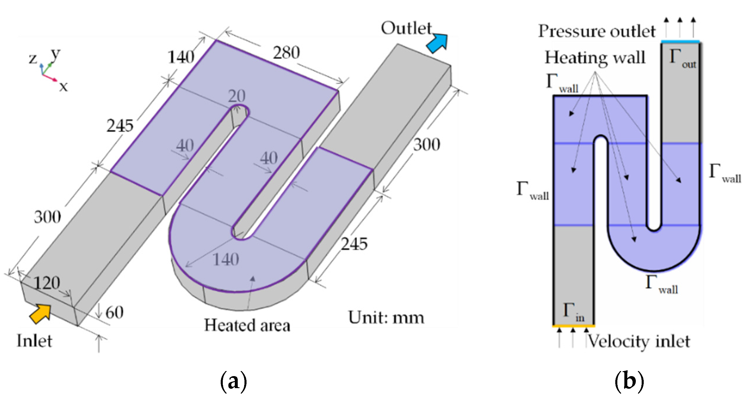
2.1. Model Description

The design model is inspired by an internal cooling channel of a turboshaft heat exchanger. The channel dimension of the numerical model in this work is consistent with the experimental serpentine cooling channel for a turbine blade with short passes, studied by Guo et al. [5]. Figure 1 illustrates the three-short-pass serpentine channel for (a) a full-scale 3D model and (b) a simplified 2D design. Each channel pass has a cross-section of 120 mm × 60 mm, yielding a hydraulic diameter (D_h) of 80 mm and an aspect ratio (AR) of 2.0. The length of all the straight passages is 245 mm, resulting in a length-to-hydraulic diameter of 3.06. Before entering the heating section, entrance and exit sections extended with a length of 300 mm are created at the channel inlet and outlet, respectively. The first turning region is designed as a rectangular shape with an inner radius of 20 mm since this region near the tip of the turbine blade suffers from a high heat load, which needs a large heat transfer area to cool. Meanwhile, the second bend near the blade platform receives a lower heat load; hence it is designed as an arc shape with outer and inner diameters of 140 and 20 mm, to reduce the total pressure loss in the channel [5].

Typically, the topology optimization requires hundreds of iterations to reach the convergence of the final optimal design. Hence, to save the cost of obtaining the optimized design, the 2D design simplified from the original 3D model is firstly used in this work [19,20,21], as demonstrated in Figure 1b. An inlet boundary condition (Γ_in) is set as uniform velocity (U_in) with a prescribed temperature (T_in). The inlet velocity is defined based on the experimental Reynolds number (Re), as follows:

$$Re=\frac{\rho U_{in}{D}_h}{\mu }$$

(1)

where ρ is fluid density and μ is dynamic viscosity.

An outlet boundary condition (Γ_out) is set as a zero static pressure (p₀). The boundary condition of the heating surfaces on the top and bottom is imposed with uniform heat flux (q₀). The remaining walls are thus set as no-slip conditions (Γ_wall) to surround the serpentine channel. Figure 1b also shows the design domains, in which all the heating regions inside design domains (Ω_id) are evolved. Meanwhile, the extended entrance and exit of the channel set as outside design domains (Ω_od) are not considered for optimization.

2.2. Thermofluid Modeling

Previous works have considered an incompressible flow for thermofluid topology optimization to design turbine blade cooling channels [24]. Moreover, it has been observed that when the Mach number is less than 0.3, the deviation of the compressible and incompressible flow can be neglected. Since the maximum bulk velocity of air in the channel is lower than 15 m/s, the Mach number is less than 0.1, then incompressible and steady-state flow are assumed throughout this work.

2.2.1. Fluid-Flow Modeling

The continuity equation and Navier–Stokes equation assuming the incompressible steady fluid are expressed as follows:

$$\rho \nabla \cdot u=0$$

(2)

$$\rho \left(\mathit{u}\cdot \nabla \right)\mathit{u}=\nabla \cdot \left[-p\mathit{I}+\left(\mu +{\mu }_T\right)\left(\nabla \mathit{u}+{\left(\nabla \mathit{u}\right)}^{*}\right)\right]+\mathit{F}$$

(3)

where u indicates the fluid velocity vector; $\nabla$ signifies the gradient operator; p denotes the pressure field; I is the identical tensor; μ_T is the turbulent dynamic viscosity; * is the transpose; and F represents the Brinkman friction term introduced by Borrvall and Petersson [34], calculated from Equation (4). Here, the body force is not exerted on the fluid outside the design domain (F = 0 in Ω_od).

$$\mathit{F}=-\left[\left({\alpha }_{u,\max }-{\alpha }_{u,\min }\right)I_u\left(\gamma \right)+{\alpha }_{u,\min }\right]\mathit{u}$$

(4)

where α_u,max is the maximum inverse permeability of the porous medium, while α_u,min is the minimum one. I_u(γ) denotes the inverse permeability interpolated function stated in Section 3.1.

From Equation (5), α_u,max can be defined depending on Darcy number (Da):

$${\alpha }_{u,\max }=\frac{\mu }{Da\cdot D_h^2}$$

(5)

2.2.2. Turbulence Modeling

As the topology optimization progressively evolves the design domain to allow material distribution, modifying the turbulence model is also necessary. In the present work, the authors modify the standard k–ε model in COMSOL by adding penalty terms to reveal the effects of turbulence on the serpentine cooling channel for topology optimization, which is modified as follows:

$$\rho \left(\mathit{u}\cdot \nabla \right)k=\nabla \cdot \left[\left(\mu +\frac{{\mu }_T}{{\sigma }_k}\right)\nabla k\right]+P_k-\rho \epsilon -{\alpha }_k\left(\gamma \right)\left(k-k_0\right)$$

(6)

$$\rho \left(\mathit{u}\cdot \nabla \right)\epsilon =\nabla \cdot \left[\left(\mu +\frac{{\mu }_T}{{\sigma }_{\epsilon }}\right)\nabla \epsilon \right]+C_{\epsilon 1}\frac{\epsilon }{k}{P}_k-C_{\epsilon 2}\rho \frac{{\epsilon }^2}{k}-{\alpha }_{\epsilon }\left(\gamma \right)\left(\epsilon -{\epsilon }_0\right)$$

(7)

The closure coefficients and all parameters in Equations (6) and (7) are described as follows:

$${\mu }_T=\rho C_{\mu }\frac{k^2}{\epsilon },\hspace{0.17em}{P}_k={\mu }_T\left[\nabla \mathit{u}:\left(\nabla \mathit{u}+{\left(\nabla \mathit{u}\right)}^{*}\right)\right],\hspace{0.17em}{C}_{\epsilon 1}=1.44,\hspace{0.17em}{C}_{\epsilon 2}=1.92,\hspace{0.17em}{\sigma }_k=1,\hspace{0.17em}{\sigma }_{\epsilon }=1$$

where P_k signifies the turbulent kinetic energy source term.

The last terms in Equations (6) and (7) are augmented to enforce k and ε to k₀ and ε₀ for the solid regions in the design domain. They are defined as follows [26]:

$${\alpha }_k\left(\gamma \right)\left(k-k_0\right)=\left[\left({\alpha }_{k,\max }-{\alpha }_{k,\min }\right)I_k\left(\gamma \right)+{\alpha }_{k,\min }\right]\left(k-k_0\right)$$

(8)

$${\alpha }_{\epsilon }\left(\gamma \right)\left(\epsilon -{\epsilon }_0\right)=\left[\left({\alpha }_{\epsilon ,\max }-{\alpha }_{\epsilon ,\min }\right)I_{\epsilon }\left(\gamma \right)+{\alpha }_{\epsilon ,\min }\right]\left(\epsilon -{\epsilon }_0\right)$$

(9)

where α_k,max and α_ε,max are the maximum limits of the penalization for k and ε, respectively, while α_k,min and α_ε,min are the minimum ones. I_k(γ) and I_ε(γ) are material interpolated functions in both Equations (8) and (9). Here, the values of α_k,min, α_ε,min, k₀ and ε₀ are assigned to zero, while the value of α_k,max and α_ε,max are set equal to the value of α_u,max. The material interpolations are detailed in Section 3.1.

2.2.3. Heat Transfer Modeling

The thermal convection–diffusion equation outside the design domain is given as follows:

$$\rho c_f\mathit{u}\nabla T-\nabla \cdot \left(k_f\nabla T\right)=0$$

(10)

where c_f denotes the fluid heat capacity, k_f indicates the fluid thermal conductivity and T is the temperature field in the serpentine channel.

In the design domain, as the distribution of the fluid and solid domains is determined after the optimization, the authors build up the energy equation by adding the functions to control the convective and conduction terms as follows:

$$\rho c_f{I}_c\left(\gamma \right)u\nabla T-\nabla \cdot \left(k_f{I}_K\left(\gamma \right)\nabla T\right)=q_0$$

(11)

where I_c(γ) is the function used to activate/deactivate the convective term for fluid (I_c(γ) = 1) and solid (I_c(γ) = 0). I_K(γ) is used to interpolate between the thermal conductivity of the fluid and the thermal conductivity of the solid (k_s). Lastly, the term q₀ indicates the constant bottom wall heat flux.

It should be noted that q₀ is the uniform heat flux applied to the heating boundaries in the 2D model. Additionally, the energy equation is weakly coupled to the fluid flow problem to obtain u; then, it substitutes the energy equation to solve T. Furthermore, the Reynolds number and heat flux applied in this work are fixed at Re = 10,000 and q₀ = 1500 W/m², respectively, because varying the velocity or the heat input in the topology optimization could change the topology of the structure in the final result [11,14].

3. Optimization Procedures

The procedure for obtaining the optimized model with lattice structures in this study is depicted in Figure 2. Firstly, the 2D simplified model, shown in Figure 1b, is topologically optimized using the boundary conditions and governing equations described in Section 2. The optimal solid domain, including the intermediate densities, is then extruded into the 3D model and interpreted with the TPMS structures. Finally, the final designs are recalculated for comparison.

3.1. Topology Optimization

In this section, the details of the topology optimization process to obtain the 2D optimized structure are presented.

3.1.1. Material Distribution

The material distribution in the density-based method described by the design variable (γ) takes a value between 0 and 1 at any point in the design domain. Here, γ = 1 denotes free flow in the channel, while γ = 0 is solid regions. The discrete 0/1 problem is relaxed to use gradient-based methods. As the material distribution takes intermediate values (0 ≤ γ ≤ 1), this relaxation requires the interpolation of transition areas. The interpolations of the fluid flow equation in the design domain are expressed in Equations (12)–(14):

$$I_u\left(\gamma \right)=q_u\frac{1-\gamma }{q_u+\gamma }$$

(12)

$$I_k\left(\gamma \right)=q_k\frac{1-\gamma }{q_k+\gamma }$$

(13)

$$I_{\epsilon }\left(\gamma \right)=q_{\epsilon }\frac{1-\gamma }{q_{\epsilon }+\gamma }$$

(14)

where q_u, q_k and q_ε are tuning parameters to control the function curvature.

For the thermal convection and conductivity, the interpolation terms I_c(γ) and I_K(γ) are calculated using solid isotropic material penalization (SIMP) [8] in Equations (15) and (16), respectively:

$$I_c\left(\gamma \right)={\gamma }^{n_c}+\left(1-{\gamma }^{n_c}\right)\delta$$

(15)

$$I_K\left(\gamma \right)={\gamma }^{n_K}+\left(1-{\gamma }^{n_K}\right)\frac{k_s}{k_f}$$

(16)

where n_c and n_K are penalization power coefficients; δ is fixed at δ = 10⁻¹⁵ to avoid numerical problems when solving Equation (11) [22].

3.1.2. Problem Formulation

In this study, minimizing the pressure loss is set as the objective function (J), while the heat transfer across the serpentine channel is constrained. In minimizing the pressure loss for the cooling channel, the power dissipation within the volume is generally selected to proceed in the optimization process since it shows the flow fluctuation in the considered domain. It provides robust convergence, and better flow uniformity can be expected when minimizing this function [11,12]. The power dissipation is expressed as follows:

$$J={\displaystyle {\int }_{\mathrm{\Omega }}^{}\left[\left(\mu +{\mu }_T\right)\left(\nabla \mathit{u}+{\left(\nabla \mathit{u}\right)}^{*}\right):\nabla \mathit{u}+\alpha \mathit{u}\cdot \mathit{u}\right]}d\mathbf{\Omega }$$

(17)

In prior works, the temperature through the boundary has been defined as another objective function to maximize heat transfer [24]. This function represents the temperature gain of fluid across the channel. Since the majority of the previous work has observed that the use of the turning vanes deteriorated the heat transfer [4,5,6], the temperature constraint (C) is thus employed to restrict the heat transfer in the present work. It is written as follows:

$$C={\displaystyle {\int }_{{\mathrm{\Gamma }}_{\mathrm{out}}}^{}T\left(\mathit{u}\cdot \mathit{n}\right)}d{\mathrm{\Gamma }}_{\mathrm{out}}$$

(18)

Here, Γ_out is the outlet boundary, and n is the normal vector. With this expression, the heat transfer in the channel can be constrained (g) as follows:

$$g=\frac{C}{C_{ref}}-1\ge 0$$

(19)

where C_ref is the reference value calculated from the conventional serpentine channel.

Hence, the mathematical optimization model is written in Equation (20):

$$\mathrm{Minimize} J={\displaystyle {\int }_{\mathrm{\Omega }}^{}\left[\left(\mu +{\mu }_T\right)\left(\nabla \mathit{u}+{\left(\nabla \mathit{u}\right)}^{*}\right):\nabla \mathit{u}+\alpha \mathit{u}\cdot \mathit{u}\right]}d\mathrm{\Omega }$$

$$\mathrm{Subject} \mathrm{to} \mathit{R}\left(\gamma ,\mathit{S}(\gamma )\right)=0$$

(20)

$$g={\displaystyle {\int }_{{\mathrm{\Gamma }}_{\mathrm{out}}}^{}T\left(\mathit{u}\cdot \mathit{n}\right)d{\mathrm{\Gamma }}_{out}}\ge C_{ref}$$

$$0\le \gamma \left(x\right)\le 1,\forall x\in {\mathrm{\Omega }}_{id}$$

where S is the vectors with discrete state fields, R indicates the residual vector function evaluated from the discretization of the governing equations, g represents inequality constraints and x denotes the design variable vector.

3.1.3. Density Filter and Projection

During the iterative process, the design variable changes independently in each cell, causing a large difference value of the design variables in the adjacent cells. In the present optimization, a partial differential equation filter [35] is adopted to mitigate such phenomena, which is defined as follows:

$$-R_{\min }^2{\nabla }^2{\gamma }_f+{\gamma }_f=\gamma$$

(21)

where γ_f signifies a smoothed design variable. R_min is a filter radius calculated by = 1.5 × maximum mesh size in the considered domain.

Additionally, a projection technique, which projects the design variable into either 0 or 1, is adopted to mitigate the intermediate results. Here, a smoothed Heaviside projection is applied as follows:

$${\gamma }_p=\frac{\tanh \left(\beta \eta \right)+\tanh \left(\beta \left({\gamma }_f-\eta \right)\right)}{\tanh \left(\beta \eta \right)+\tanh \left(\beta \left(1-\eta \right)\right)}$$

(22)

where γ_p is the projected design variable, β is a parameter used to control the steepness of the projection, and η denotes the projection threshold, fixed at η = 0.5 in this study.

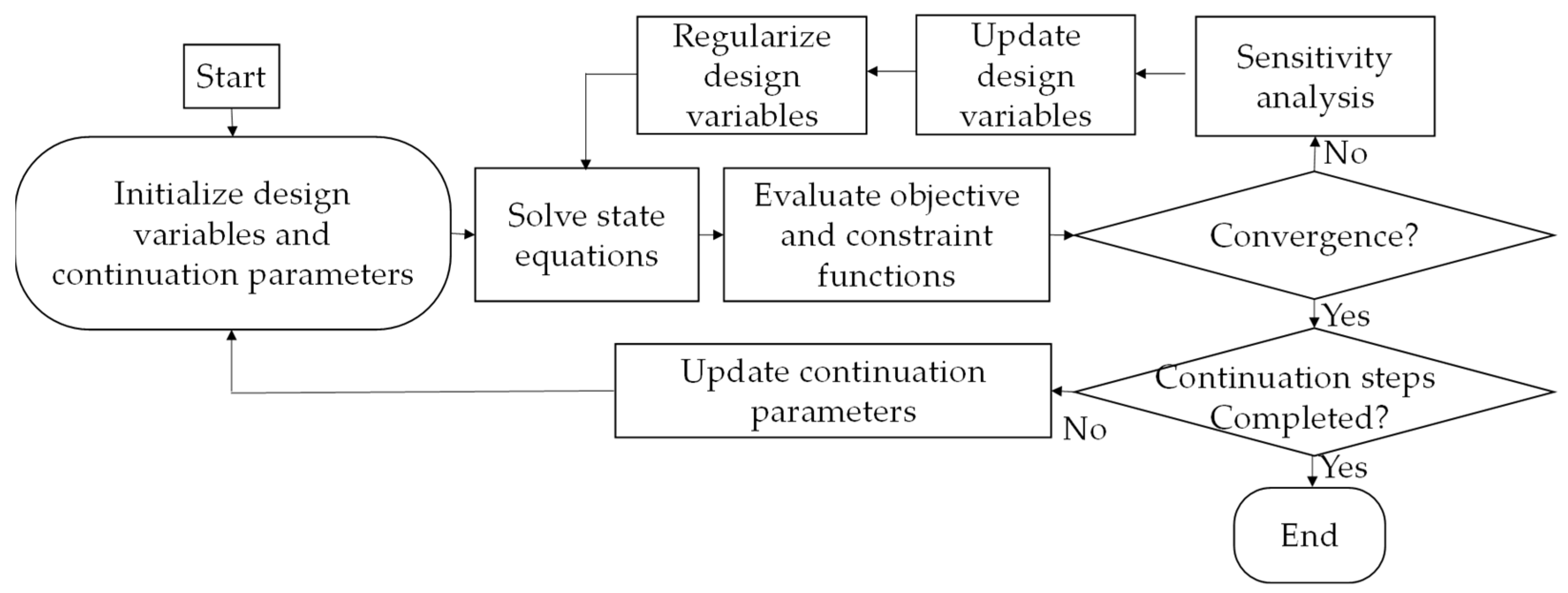
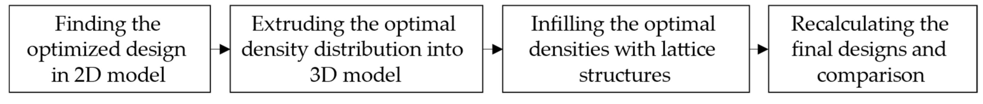
3.1.4. Summary of Topology Optimization Process

The present study uses COMSOL Multiphysics to run the topology optimization process. The flow chart of the topology optimization process is demonstrated in Figure 3. After the design variables and the parameters are initialized, the governing equations are solved to attain physical variable fields. The objective and the constraint functions are then computed. If the convergence criterion is not achieved, the sensitivity is computed by the adjoint method to obtain the gradient information. The design variable field is then updated using GCMMA and regularized. When the constraint is achieved, and the relative change in the objective is less than 10⁻⁴, or after every 100 iterations, the optimization proceeds to the next continuation steps. The continuation approach is used to avoid the low-quality local minima result and ease the convergence in this optimization process [18]. Eventually, the optimization is considered to be completed when all the continuation steps are computed.

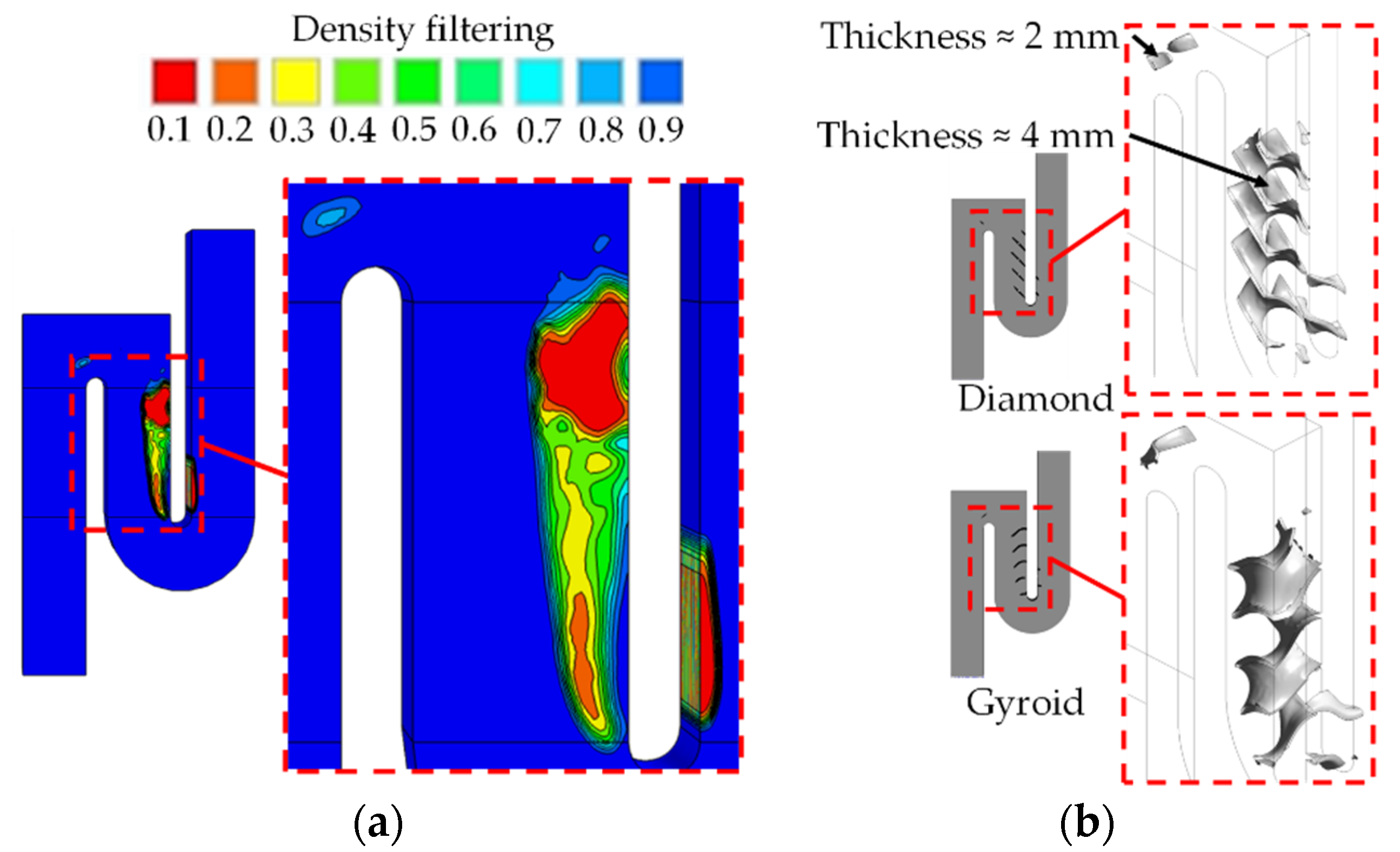
3.2. Infilling Lattice Structures

After obtaining the 2D optimized model, the optimal solid domain within the channel, including intermediate results generated by the conventional topology optimization, is extruded into the 3D model and replaced by TPMS structures. The TPMS networks are used to infill the extruded optimized model with a range of thickness according to the optimal density results. Here, the diamond and gyroid-sheet structures, as shown in Figure 4, are chosen to replace the solid domains and intermediate results of the extruded optimized model due to their excellent thermal performance [31,32,33]. The final designs are then recomputed.

4. Results and Discussion

In this section, two main parts are presented. For the topology optimization, the problem setup and 2D simplified model validation are detailed in the first part. The optimal density distribution in the 2D optimized model is extruded into the 3D domain and fulfilled with the TPMS structures. The final designs are then recalculated and validated in the second part. The pressure drop, heat transfer and temperature uniformity are compared with the baseline serpentine channels.

4.1. 2D Optimization

4.1.1. Validation of the 2D Model

Since the 3D channel is simplified into the 2D model to reduce the computational cost for topology optimization, the accuracy of the stated variable field obtained from 2D calculations should be satisfied [19]. Air and copper are selected in this work for fluid and solid properties for the simulation. The boundary conditions and governing equations explained in Section 2 are used to compute the flow, turbulence effect and heat transfer. It should be marked that in COMSOL, the out-of-plane heat flux (q₀) in the 2D model is equivalent to the uniform heat flux boundary in the 3D system.

The mesh system of the 2D and 3D models is demonstrated in Figure 5. It is suggested that the boundary layer mesh evolves during the optimization for the accurate turbulence calculation, or the mesh should be fine enough to obtain accurate and reliable results. The extra-fine mesh setting at 42,468 elements, containing mainly triangle element type, is thus generated for all 2D models, as shown in Figure 5a. Meanwhile, for the 3D model, the tetrahedral mesh is generated, and the boundary layer mesh with a prism shape is employed in the wall regions. The fine mesh system is selected at 2.38 million elements, as shown in Figure 5b.

To verify the discrepancy between the 2D and 3D models, averaged values of the pressure, velocity and temperature at 12 different positions are plotted in Figure 6. In all 2D cases, the results are averaged from 12-cut lines, whereas in all 3D cases, the outcomes are extracted from the planes, then averaged. Overall, the 2D results have similar trends to the 3D ones for all variables. The pressure values in Figure 6a and velocity magnitudes in Figure 6b for the 2D model are lower than in the 3D model, while the temperature values in Figure 6c are opposite. The 2D model overestimates the temperature by about 0.4%–2.5%, and the average error value is 1.6%. The temperature discrepancy between the 2D and 3D models can attribute to the limitation of a pseudo-3D model, which has also been observed in several investigations [13,19]. However, the temperature distributions that slightly decreased along the channel path are well estimated, providing similar trends among them. The variations can be acceptable for the optimization process. Therefore, comparing results with the 3D numerical model, the 2D model can be accurately employed to perform topology optimization in this work.

4.1.2. Optimized Structure

The initial design is a uniform density field of γ₀ = 0.6. The model is evaluated through the continuation parameters, as given in

Table 2. Parameters used in the 2D topology optimization process.

Parameter	Da	β	η	qu	qk	qε	nc	nK
Value	10−4–10−6	1.5–16.0	0.5	0.1–10	0.001	0.1	3–5	3–5

, to find the optimal structure. After the simulation, the design converges to the optimized structure, as presented in Figure 7. It can be noticed that the model leaves the intermediate fields to satisfy the temperature constraint by distributing the material in the channel. The intermediate results are due to the high conductivity difference between the copper and air used in this work [19]. For the 2D optimized design, the total pressure loss between inlet and outlet boundaries decreases by about 33.9% compared to the original 2D model, while the constraint temperature in the channel is maintained.

The optimal density distribution within the 2D optimized channel, including intermediate results generated by conventional topology optimization, is extracted with ranges of density filtering from 0.1 to 0.9 and extruded into the 3D model, as shown in Figure 8a. The TPMS structures are then used to infill with a range of thickness between 2–4 mm. The lowest thickness of 2 mm is specified at the density filtering of 0.9, and the thickness is increased accordingly, reaching the highest thickness of 4 mm at the density filtering of 0.1, as demonstrated in Figure 8b. The thickness range is selected based on the printable capability in an actual scale of the cooling channel for a gas turbine blade. Here, the single unit cell size of the diamond- and gyroid-sheet structures is 120 × 120 × 120 mm³.

4.2. 3D Model Comparisons

In this section, the optimized model extracted with a density filtering of 0.5 (TO model) is also included to compare with the baseline channel. All models and the boundary conditions are shown in Figure 9. These models are applicable at the Reynolds number Re = 10,000 and heat flux q₀ = 1500 W/m² according to the design settings in the conventional topology optimization, as mentioned in Section 2. For all cases, the channel dimensions are consistent with the baseline serpentine channel, as described in Figure 1a. The inlet and outlet boundaries are the same as the baseline channel. Here, the red zones are treated by the uniform heat flux, including the top, bottom and extruded areas from the optimization and TPMS structures. The remaining surfaces are set as no-slip walls.

The flow and heat transfer for all models in this section are simulated using the commercial CFD solver ANSYS FLUENT 18.0, which provides lower computational costs and consumes lesser computer memory for 3D complex cooling channels than COMSOL. The overview of mesh systems for the optimized model with the diamond-sheet structure is demonstrated as an example in Figure 10. The hybrid mesh involving tetrahedron and prism elements is created to discretize the entire domain. The tetrahedron meshes are finely dense in the small- and high-curvature regions, while the boundary layer meshes with a prism shape are used near the no-slip walls. The meshes near the wall are refined to ensure that y+ values are less than one.

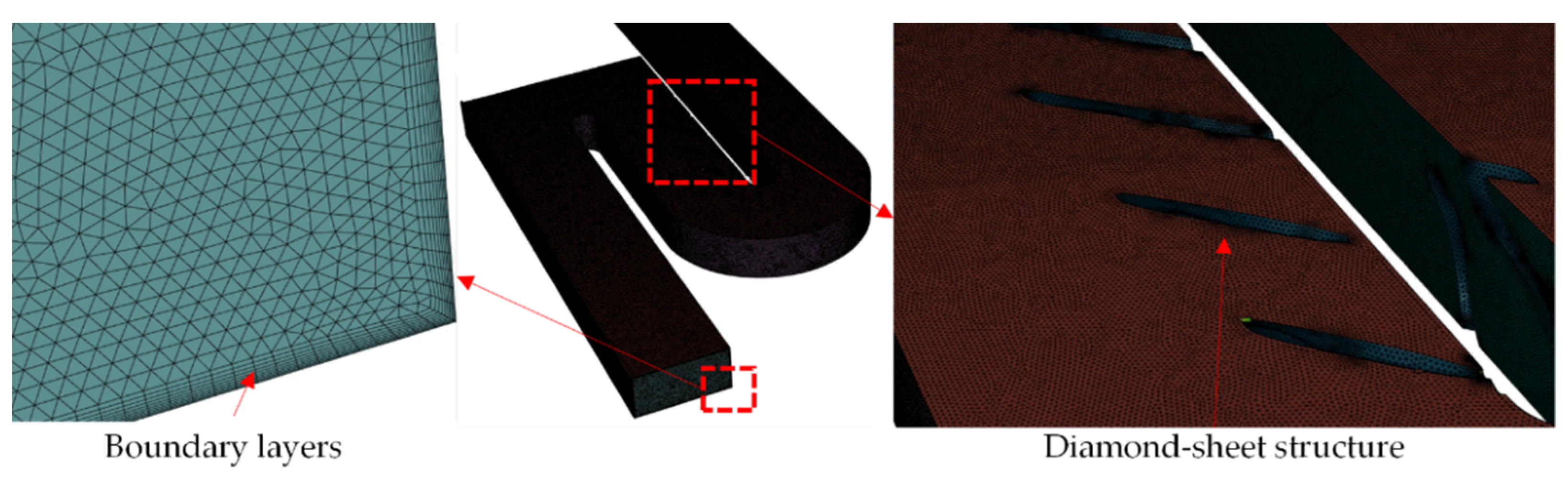
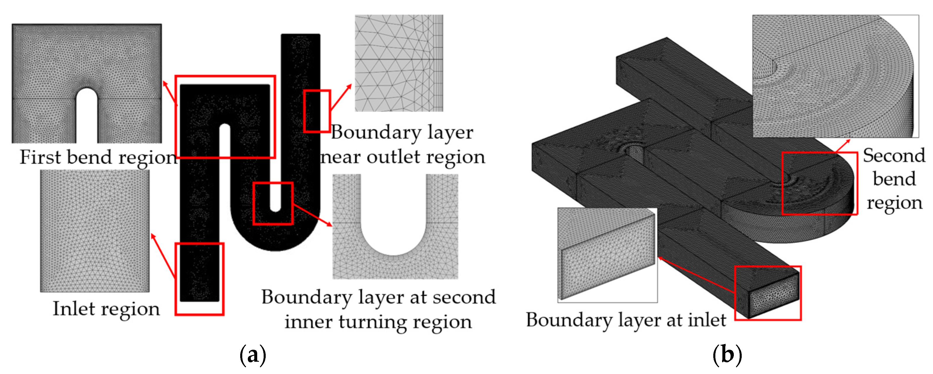
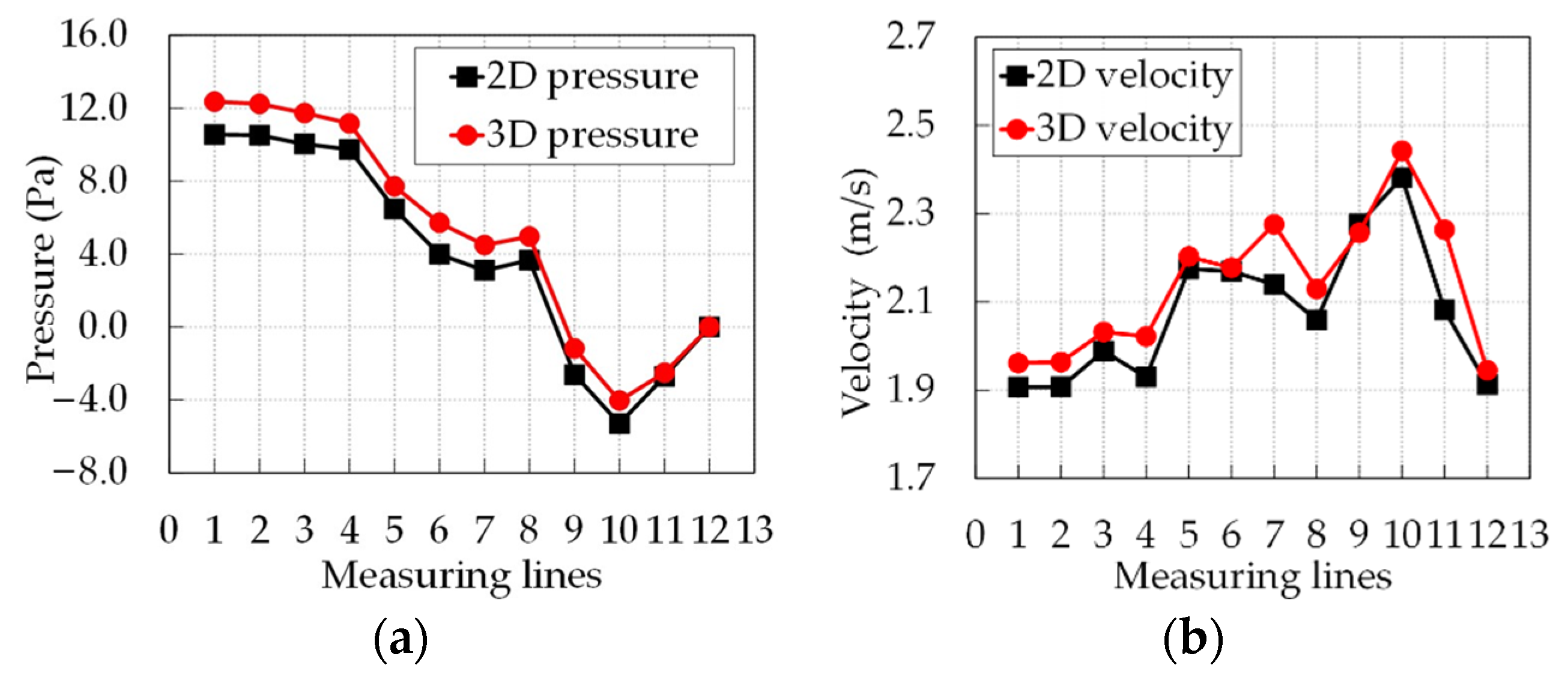
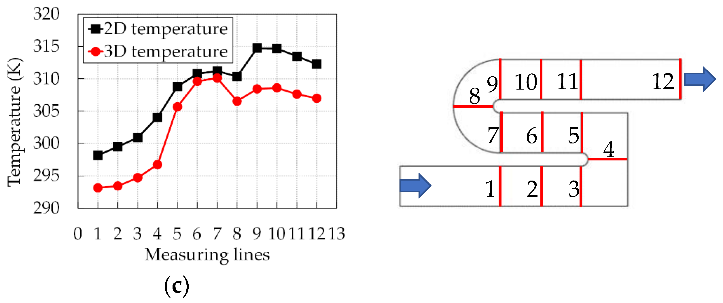
4.2.1. 3D Model Validation

For the validation, the conventional three-short-pass smooth channel investigated by Guo et al. [5] is used as the referee design. The SIMPLEC algorithm is utilized for the pressure–velocity coupling, and the second-order upwind method is adopted. The convergence criterion is less than 10⁻⁴ for the continuity, velocity and turbulence quantities and less than 10⁻⁶ for the energy equation [5].

Three sets of the meshes at 4.95, 7.31 and 11.6 million elements are simulated to check mesh independence for the baseline channel. The numerical results are steady and converge to a certain value as the mesh elements increase. The grid convergence index (GCI) [36] is evaluated using the spanwise-averaged surface temperature to estimate the numerical accuracy of the mesh at 7.31 million, as demonstrated in Figure 11. The line denotes the highest mesh solution, while the red bars represent the error. It is found that the maximum error of the samples is less than 0.5%, and the overall GCI value on the spanwise-averaged temperature is about 0.1%, which indicates that the numerical results are independent of the meshes. Therefore, the mesh element is selected at 7.31 million for the baseline serpentine channel, while this mesh setting is also used for the other models.

In order to select the turbulence model with the highest accuracy, several Reynolds-averaged Navier–Stokes equations (RANS), i.e., SST k–ω, realizable k–ε and RNG k–ε, are executed and compared with the baseline serpentine channel. SST means the shear stress transport turbulence model, and RNG denotes renormalization group methods. Here, the globally averaged Nusselt number of each pass ($\overline{\overline{Nu}}$) is used to compare the heat transfer with the experimental data from Guo et al. [5]. It can be evaluated as follows:

$$\overline{\overline{Nu}}=\frac{Q_{tot}}{A_w\Delta T}\frac{D_h}{k_f}$$

(23)

where Q_tot denotes the total heat transfer, A_w is the wetted area, and ΔT signifies the log mean temperature difference of the heating wall, calculated as follows:

$$\Delta T=\frac{\left(T_w-T_{in}\right)-\left(T_w-T_{out}\right)}{\ln \left(\frac{T_w-T_{in}}{T_w-T_{out}}\right)}$$

(24)

where T_w is the average wall temperature, while T_in and T_out are the inlet and outlet fluid temperatures.

The globally averaged Nusselt number simulated from different turbulence models for the baseline serpentine channel at the Reynolds number of 10,000 is shown in Figure 12. It should be noted that Guo et al. [5] have found that the SST k–ω turbulence model could accurately simulate the heat transfer of the three-pass channel with ribs. This is because the SST k–ω turbulence model captures well the reattachment flow from the ribbed walls. However, in this work, SST k–ω and RNG k–ε considerably overestimates the results in the second pass by 25.9% and 21.4%, respectively. Meanwhile, the average Nusselt number simulated using realizable k–ε agrees well with the experimental results for all smooth passages due to correctly predicting the large recirculation flow. The mean error deviates by about 10.7% compared to the experimental data. Hence, the realizable k–ε turbulence model with enhanced wall treatment is selected to simulate all models in this study.

4.2.2. Pressure Loss

The relative pressure coefficient (C_p) is employed to characterize the pressure loss from different models. The relative pressure coefficient along the channel flow path is calculated as follows:

$$C_p=\frac{p_{loc}-p_{ref}}{\rho U_{in}^2/2}$$

(25)

where p_loc is the local static pressure at measuring points and p_ref indicates the pressure value at the channel inlet.

The relative pressure coefficient at three different locations at the Reynolds number of 10,000 is demonstrated in Figure 13. In the first pass, as the structure for all models is the same without changing from the baseline channel, the values are comparable because the coolant flows smoothly with minor flow resistance. The losses are higher when the coolant enters the second and third passes. Here, the baseline serpentine channel causes the highest losses, followed by the TO model with the gyroid-TPMS structure. In contrast, the TO model provides the lowest values, which are lower than the baseline model by 14.5% and 44.3% for the second and third passages.

The friction factor calculated to compare the total pressure loss in the channel can be expressed as follows:

$$f=\frac{2\Delta p{D}_h}{\rho U_{in}^{2}L}$$

(26)

where Δp is calculated from the pressure at the inlet boundary minus the pressure at the outlet boundary. L is the total length of the serpentine cooling channel.

The friction factor for all models at the Reynolds number of 10,000 is compared in Figure 14. All cases cause lower friction loss than the baseline channel, and the TO model provides the lowest value. It can be observed that the TO model with diamond- and TO model with gyroid-TPMS structures cause slightly higher friction loss than the TO model attributed to their complex curvatures. Compared to the baseline channel, the TO model, TO model with diamond- and TO model with gyroid-TPMS structures show a friction loss reduction of 38.0%, 30.8% and 19.0%, respectively.

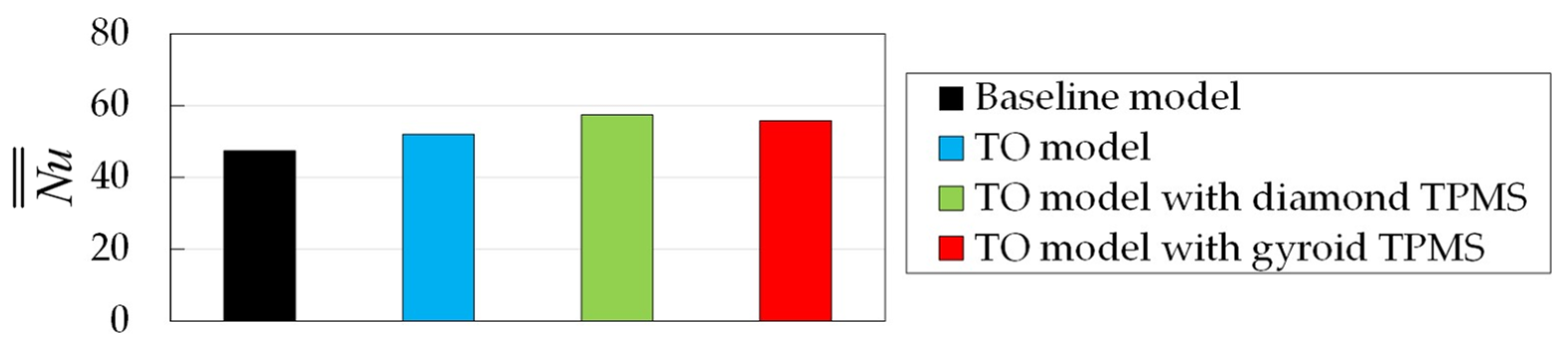
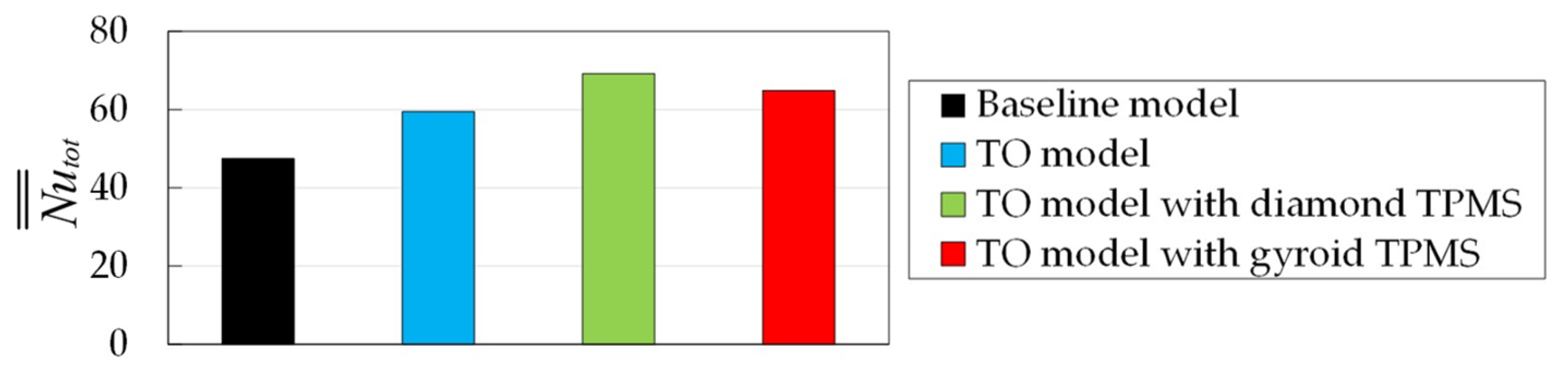
4.2.3. Heat Transfer

The globally average Nusselt number, including two turning regions, at the Reynolds number of 10,000 is presented in Figure 15. It is evident that all topology optimization models provide higher heat transfer than the baseline channel, particularly in the TO model with the diamond-TPMS structure. This result is because the heat transfer is constrained during the optimization, and the heat transfer is further increased when interpreting the intermediate results with the TPMS structures. The globally averaged Nusselt number in the TO model, TO model with diamond- and TO model with gyroid-TPMS structures are higher than in the baseline channel by about 9.6%, 21.1% and 17.6%, respectively.

The total Nusselt number (${\overline{\overline{Nu}}}_{tot}$) presents the total heat transfer performance based on the flat base heating area. The total Nusselt number includes the heat transfer contribution from all wetted surfaces, as the total heat transfer is experienced by the turbine blade’s suction and pressure walls, and it is calculated as follows:

$${\overline{\overline{Nu}}}_{tot}=\overline{\overline{Nu}}\left(\frac{A_w}{A_h}\right)$$

(27)

where A_h is the flat heated area.

It is noted that the total wetted area of the TO model, TO model with diamond- and TO model with gyroid-TPMS structures are increased by 8.5%, 15.6% and 13.3% compared to the baseline channel. The total Nusselt number at the Reynolds number of 10,000 is shown in Figure 16. The total Nusselt number is higher than the globally averaged Nusselt number, particularly in the TO model with the diamond-TPMS structure. This substantial increase is because the diamond-sheet structure has a larger contact area than the TO model curvature and the gyroid-sheet structure. The total Nusselt number for the TO model, TO model with diamond- and TO model with gyroid-TPMS structures increases by 25.3%, 45.8% and 36.6%, respectively, compared to the baseline channel.

To show the heat transfer enhancements in the serpentine channel, the Dittus–Boelter equation [37] is employed to normalize the globally averaged and total Nusselt numbers, defined as follows:

$${\overline{\overline{Nu}}}_0=0.023R{e}^{0.8}P{r}^{0.4}$$

(28)

where Pr is the Prandtl number, and the value of Pr for the air in this study is 0.7.

The globally averaged and total heat transfer enhancements at the Reynolds number of 10,000 are presented in Figure 17a,b, respectively. The enhanced heat transfer is observed for all models since the serpentine channels generate high heat transfer, particularly from the first turning region. Among the comparative models, the heat transfer enhancement is more evident for the TO model with diamond-TPMS structure since this model considerably increases total heat transfer in the channel.

4.2.4. Thermal Performance

To compare the thermal performance of the serpentine cooling channel, the heat transfer performance requires an assessment after involving friction loss. In this study, the thermal performance of the serpentine channels can be calculated as follows:

$$TP=\frac{{\overline{\overline{Nu}}}_{tot}/{\overline{\overline{Nu}}}_0}{{\left(f/f_0\right)}^{1/3}}$$

(29)

where f₀ is the Blasius correlation, defined in Equation (30):

$$f_0=0.316R{e}^{-0.25}$$

(30)

The thermal performance for all cases at the Reynolds number 10,000 is presented in Figure 18. It is evident that the baseline serpentine channel shows the lowest thermal performance due to causing the highest pressure loss and lowest heat transfer in the channel. Meanwhile, the TO model with the diamond-TPMS structure exhibits the highest value because the optimized curvatures help minimize the pressure loss in the serpentine channel, while the diamond-sheet structure enhances high heat transfer. The thermal performance for the TO model, TO model with diamond- and TO model with gyroid-TPMS structures improves by 47.0%, 64.8% and 46.5%, respectively, compared to the baseline channel.

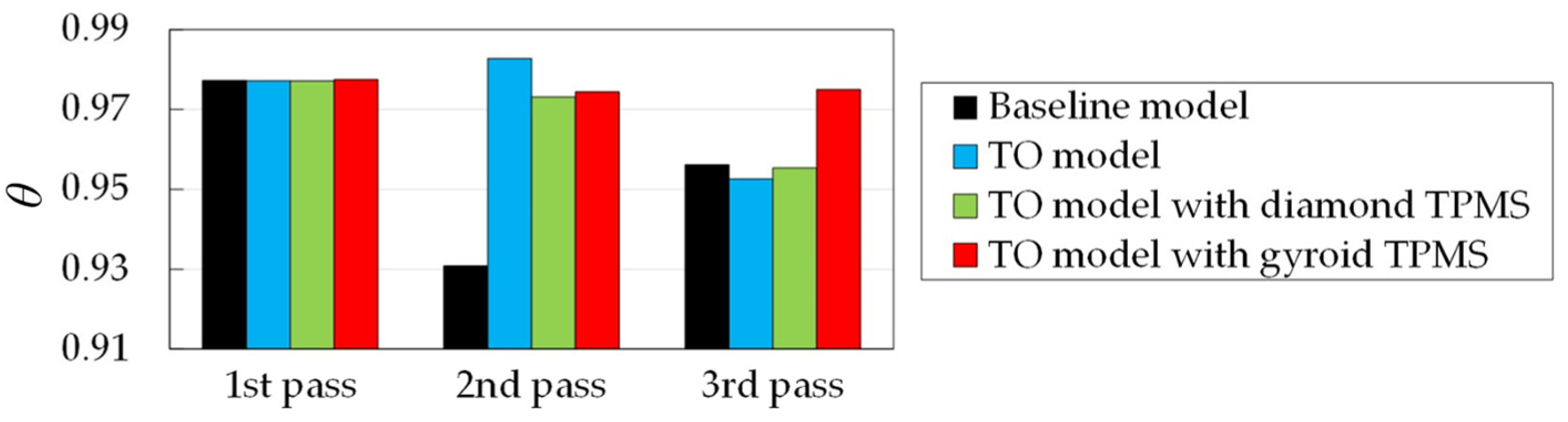
4.2.5. Temperature Uniformity

The high temperature difference between leading and trailing surfaces generated in the gas turbine channel is observed when the channel rotates at high speed [1,2]. It is essential to be concerned about the temperature uniformity that affects the temperature difference on the surface. The uniformity index of temperature (θ) is introduced in this section to determine surface temperature uniformity. It can be calculated as follows:

$$\theta =1-\frac{{\displaystyle \sum _{i=1}^n\left|T_i-T_{avg}\right|}}{2T_{avg}{A}_h}$$

(31)

where T_i denotes the local temperature, and A_i is the local area. T_avg is the average temperature of the considered region, calculated as follows:

$$T_{avg}=\frac{1}{A_p}{\displaystyle \sum _{i=1}^n{T}_i{A}_i}$$

(32)

The uniformity index of surface temperature for all serpentine channels at the Reynolds number of 10,000 is presented in Figure 19. In the first pass, all cases exhibit comparable values, while the uniformities drastically decrease in the second pass for the baseline model. These negative results are due to the strong turning effect at the first rectangular bend, causing nonuniform flow distribution throughout the second pass [5]. However, the uniformities are improved in the TO model, TO model with diamond- and TO model with gyroid-TPMS structures owing to the curvatures that manipulate smoother flow distributions. For all optimized models, the temperature uniformity on the surface improves by about 4.5%–5.6% in the second passage and 0.4%–2.0% in the third passage, superior to the baseline channel.

In short, the optimized model infilled with the diamond-sheet structure shows the best thermal performance because it provides low pressure loss and enhances the highest heat transfer. This structure also improves the temperature uniformity throughout the channel compared to the baseline model. Therefore, this study selects the TO model with diamond-TPMS structure as the optimal serpentine channel.

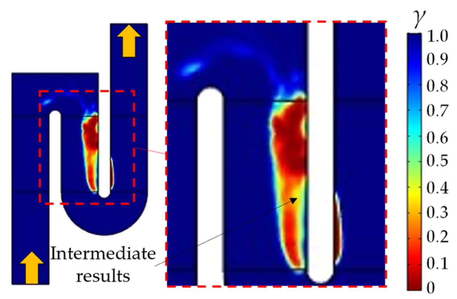
4.3. Detailed Flow and Heat Transfer Characteristics of the Optimal Serpentine Channel

According to the analysis of the pressure loss, heat transfer and temperature uniformity in Section 4.2, the optimized serpentine channel with diamond-sheet structure is selected to be the optimal model, and the detailed flow and heat transfer characteristics are demonstrated and compared to the baseline serpentine channel.

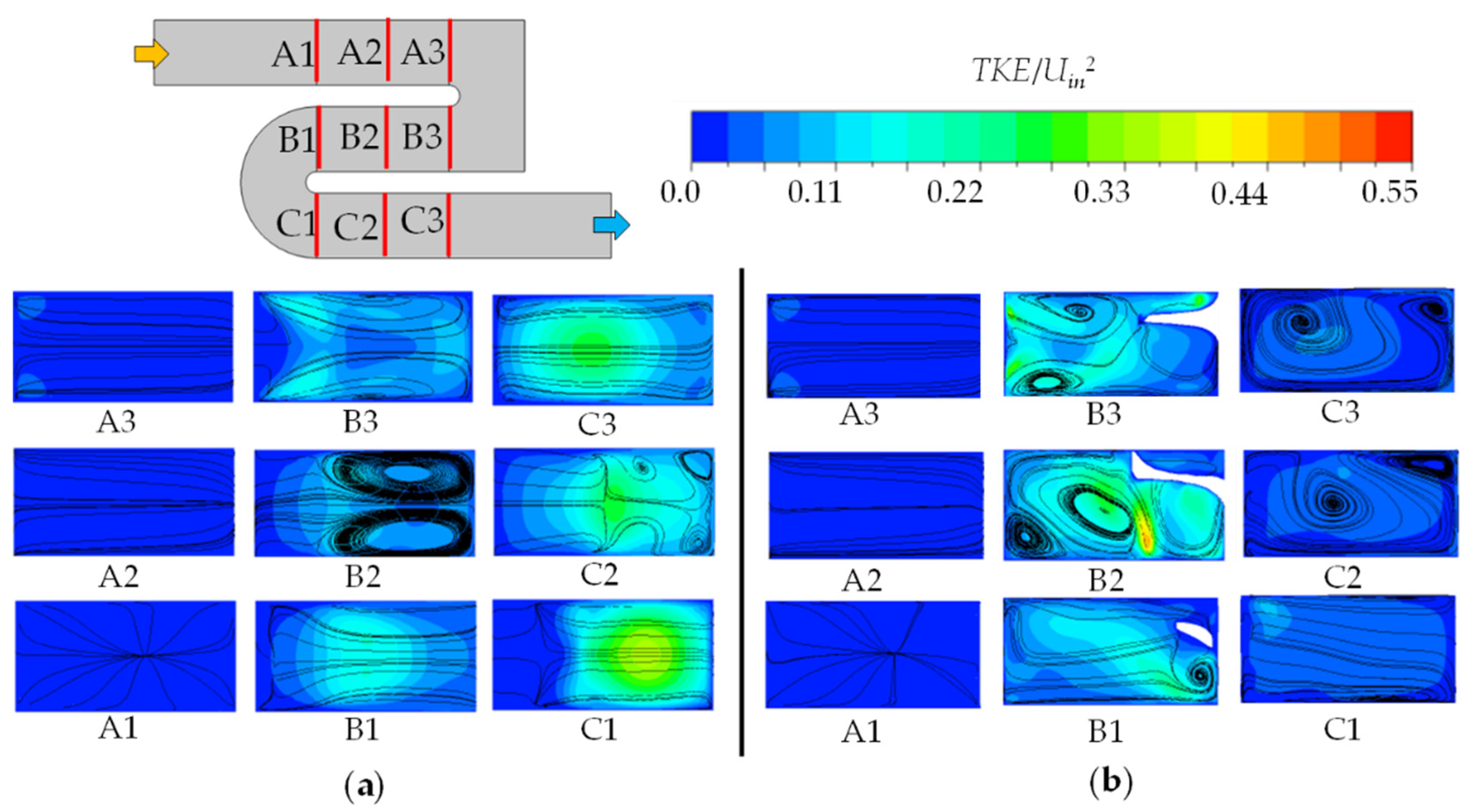
4.3.1. Flow Characteristics

The velocity distributions and streamlines on the middle section (Z = 30 mm) of the serpentine channel at the Reynolds number of 10,000 are shown in Figure 20 for (a) the baseline channel and (b) the TO model with diamond-TPMS structure. It is clearly seen that for the baseline serpentine channel, the large recirculation flow is generated at the second bend region and third passage. The high velocity can be observed at the outer wall of the third passage. These phenomena cause nonuniform distribution of the flow. Meanwhile, the recirculation flow in the TO model with the diamond-TPMS structure is eliminated, as seen in Figure 20b. The curvature in this model induces the coolant to flow near the inner wall of the second passage. The flow in the diamond-sheet structure is also distributed evenly, leading to a more uniform velocity distribution throughout the channel.

The pressure distribution on the middle section of the channel at the Reynolds number of 10,000 is demonstrated in Figure 21 for (a) the baseline model and (b) the TO model with diamond-TPMS structure. For the baseline channel, the high-pressure loss emerges in the two bend regions, which could be attributed to the generation of the Dean’s vortices [5]. However, after inserting the diamond-sheet structure into the optimized serpentine channel, the pressure loss is significantly reduced. It can be observed that the pressure loss is reduced, particularly in the second passage inside the diamond-sheet structure, and the area of low pressure continues to the third passage. The TO model with the diamond-TPMS structure manipulates the fluid well, reducing the recirculation flow, which lowers the total pressure loss in the serpentine channel.

The flow mechanisms and turning effects can be discussed with the dimensionless turbulent kinetic energy (TKE/U_in²) and streamlines on different cross-sections of the serpentine channel, as presented in Figure 22. For both models, the turbulent kinetic energy and streamlines exhibit the same characteristics in the first passage. The higher turbulent kinetic energy values can be observed in the second and third passages.

For the baseline model, as shown in Figure 22a, the Dean’s vortices can be observed on the outer wall when the fluid enters the second passage on plane B3. These vortices are prominent in plane B2, while the fluid mixes at the end of the second passage, resulting in high turbulent kinetic energy in the middle region. The coolant turning into the third passage further increases the turbulent kinetic energy and continues until it leaves the channel, as seen on planes C1–C3. Even though the strong mixing flow could enhance high heat transfer, this effect causes substantial differences in the flow distribution, eventually leading to non-uniform heat transfer in the channel.

For the TO model with the diamond-TPMS structure, as shown in Figure 22b, the Dean’s vortices at the inner wall, as found in the baseline model, are diminished because the large solid volume of the diamond-sheet structure distributes the flow in the second passage, as demonstrated on planes B3–B1. However, the high turbulent kinetic energy areas can be observed. The main coolant is forced to flow along the curvature of the diamond-sheet structure, intensifying high turbulent kinetic energy. Moreover, the complex flow generated inside the diamond-sheet structure expands large regions of high turbulence. The turbulent kinetic energy in the third passage is also more uniform than in the baseline model. These phenomena in the TO model with the diamond-TPMS structure lead to higher heat transfer and better uniformity than in the baseline channel.

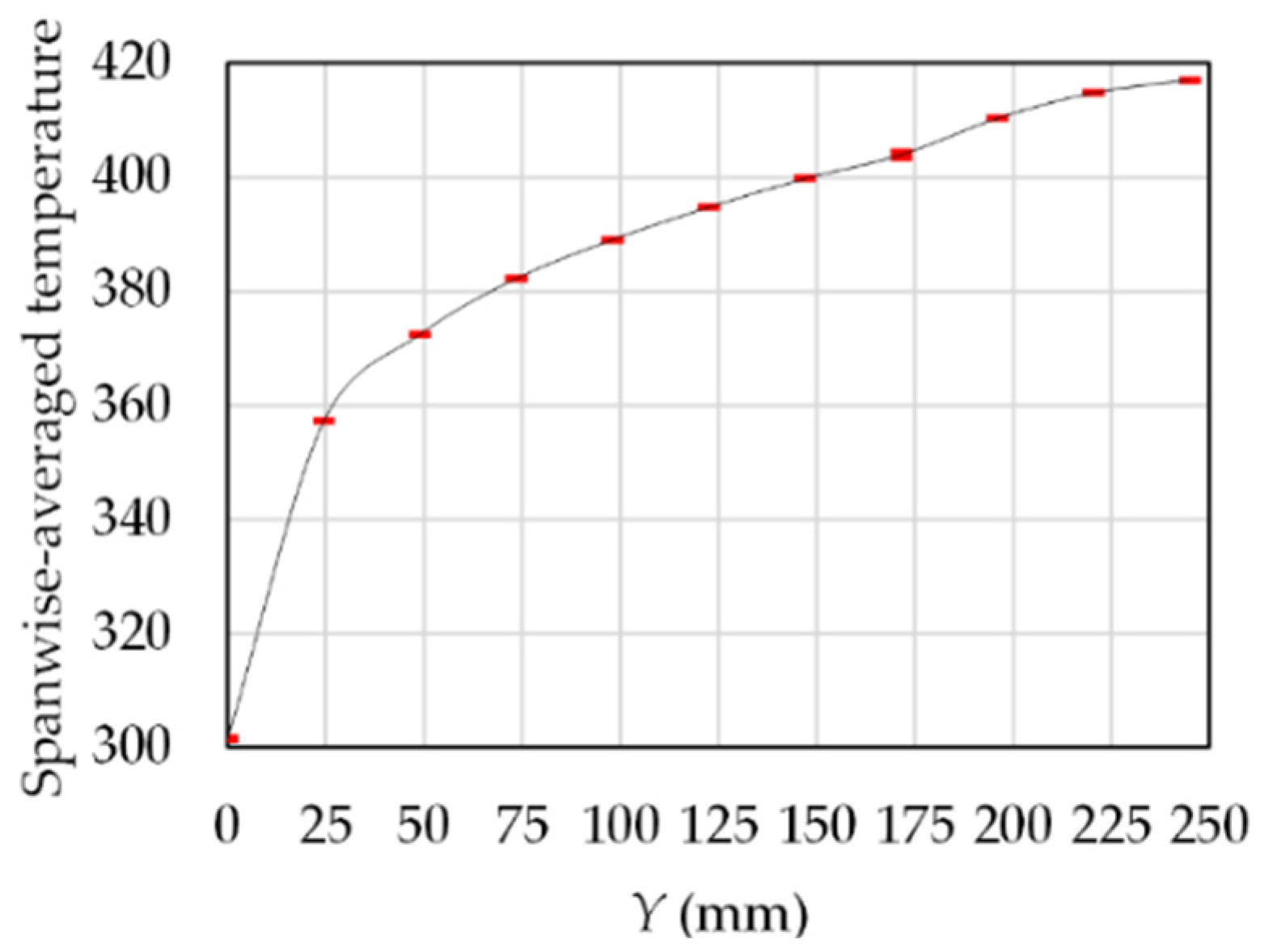
4.3.2. Heat Transfer Characteristics

The local Nusselt number (Nu) is employed to analyze the surface heat transfer. The local Nusselt number is evaluated from the local heat transfer coefficient based on the local wall heat flux and the local temperature difference between the wall and the corresponding fluid bulk temperatures. The Nusselt number contour at the Reynolds number of 10,000 is illustrated in Figure 23 for (a) the baseline model and (b) the TO model with diamond-TPMS structure. For the baseline channel, as presented in Figure 23a, it can be clearly seen that the low Nusselt number region near the inner wall of the second passage is considerably expanded due to the large recirculation flow. However, this low heat transfer disappears in the TO model with diamond-TPMS structure, particularly in the second passage, as shown in Figure 23b. The high-value areas can also be observed inside the diamond-sheet structure because the curved interconnected walls generate impingement flow on the surface, as shown in the enlarged view. The average heat transfer at the second passage increases by 69.8% compared to the baseline model. Moreover, as the recirculation flow is eliminated due to the curvature of the diamond-sheet structure in the second and third passages of the TO model with diamond-TPMS structure, more uniform distributions of high heat transfer can be observed. The uniform heat transfer distributions are beneficial to mitigate the local thermal stress in the gas turbine blade.

5. Conclusions

In this work, the concept of density-based topology optimization is utilized to design the serpentine cooling channel under turbulent flow. In the topology optimization, the penalization terms are added to the k–ε turbulence model to reveal the turbulence effects. The functions to activate/deactivate the convective and conduction terms in the energy equation are also carried out. The main objective is to minimize the pressure drop while maintaining heat transfer. The 2D simplified models are topologically optimized. The optimized solution, including the intermediate results, is then extruded into the 3D system and infilled with TPMS structures. The final models are resimulated and validated to compare with the baseline serpentine channel. The main conclusions are drawn as follows:

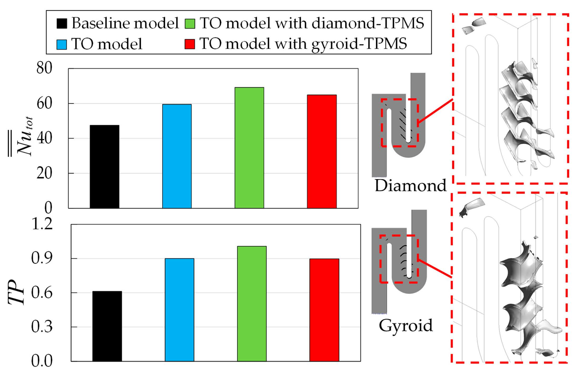
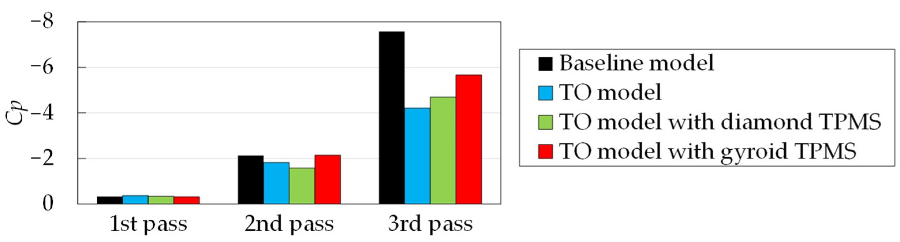
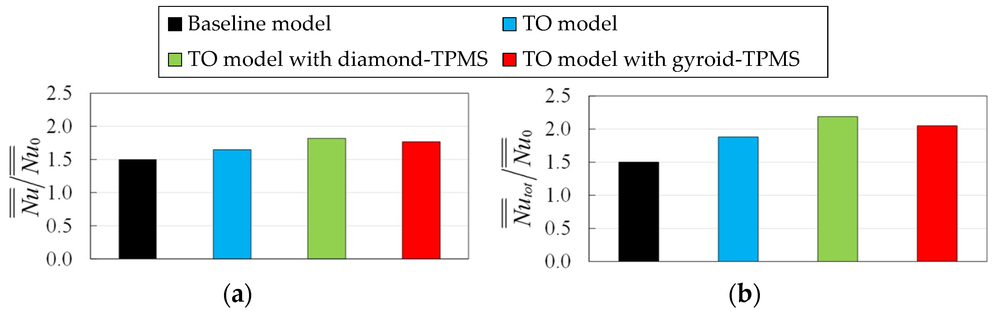
• The conventional topology optimization model achieves a lower pressure loss and provides higher heat transfer than the baseline channel. Infilling the diamond- and gyroid-sheet structures in the optimal solution, including the intermediate results of the conventional topology optimization model, further enhance high heat transfer and maintains lower pressure loss than the baseline channel.
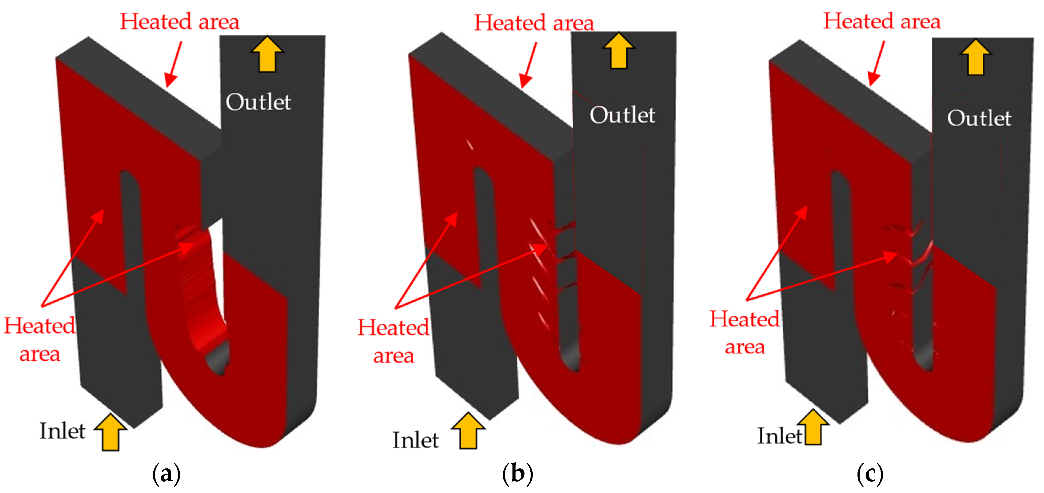
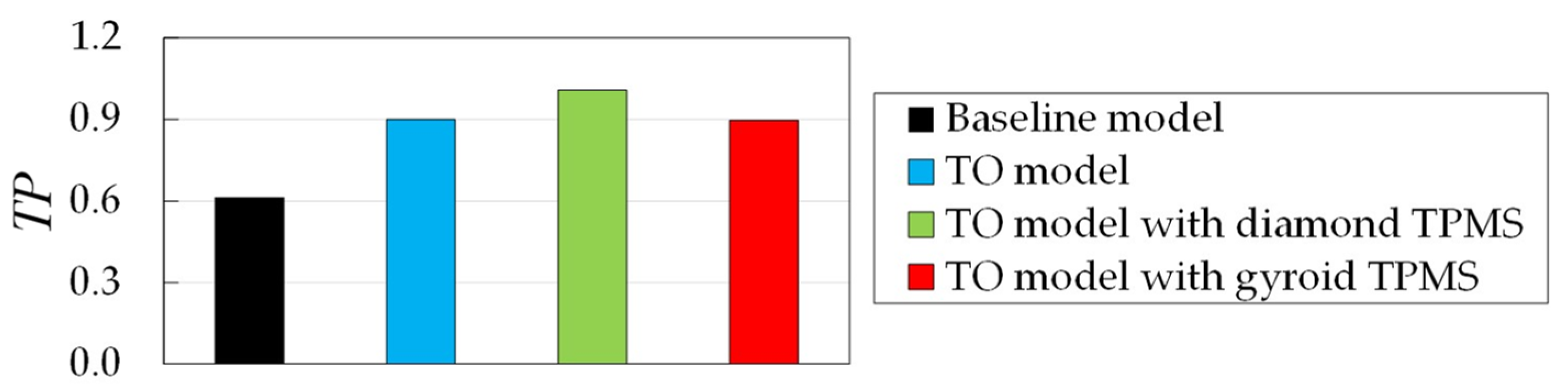
• The 3D optimized models with the TPMS structures provide lower pressure loss by about 19.0%–30.8% and higher total heat transfer by 36.6%–45.8%, compared to the 3D baseline channel. The optimized mode infilled with the diamond-TPMS structure is selected as the optimal serpentine channel in this study since it provides the best thermal performance, up to 64.8%, superior to the baseline channel. The temperature uniformity on the surface is also improved, particularly in the second passage.
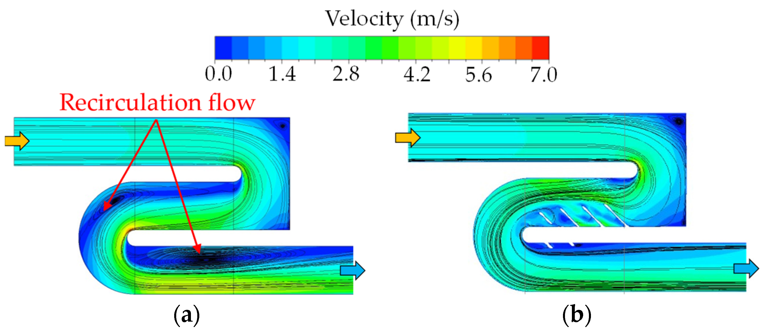
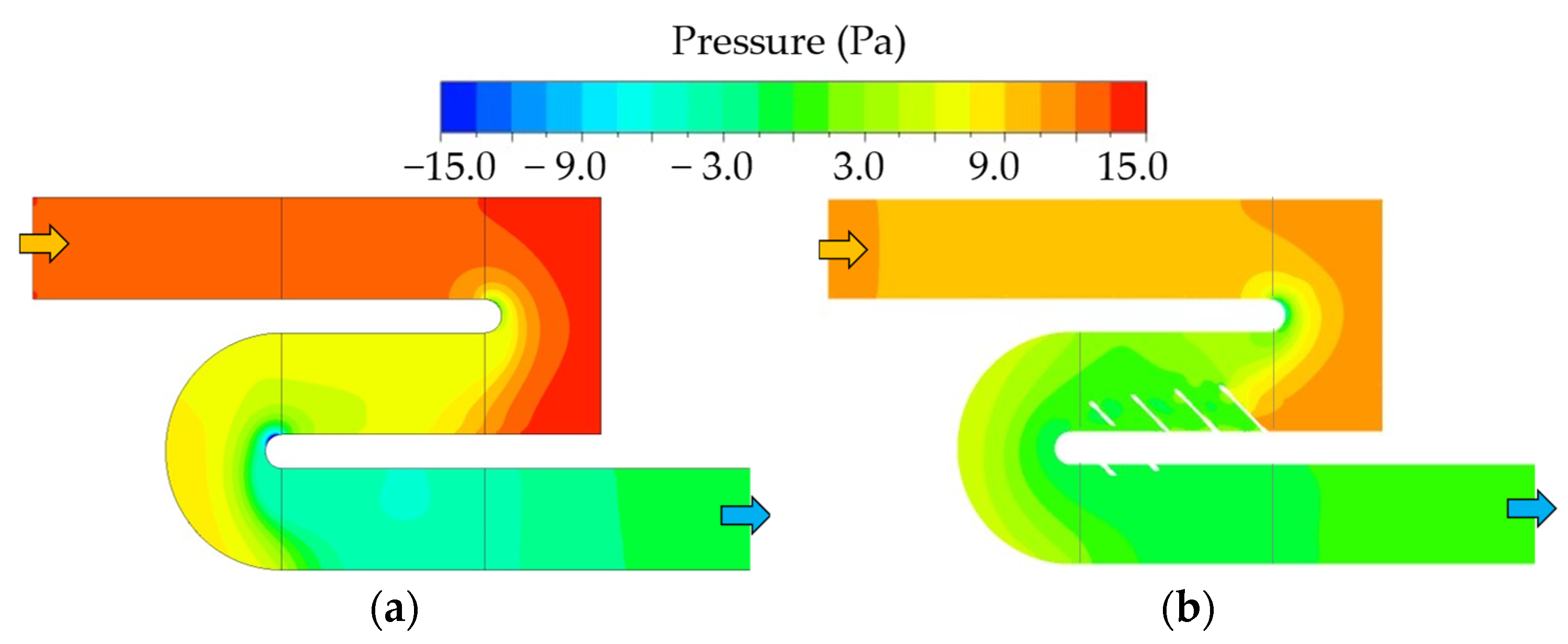
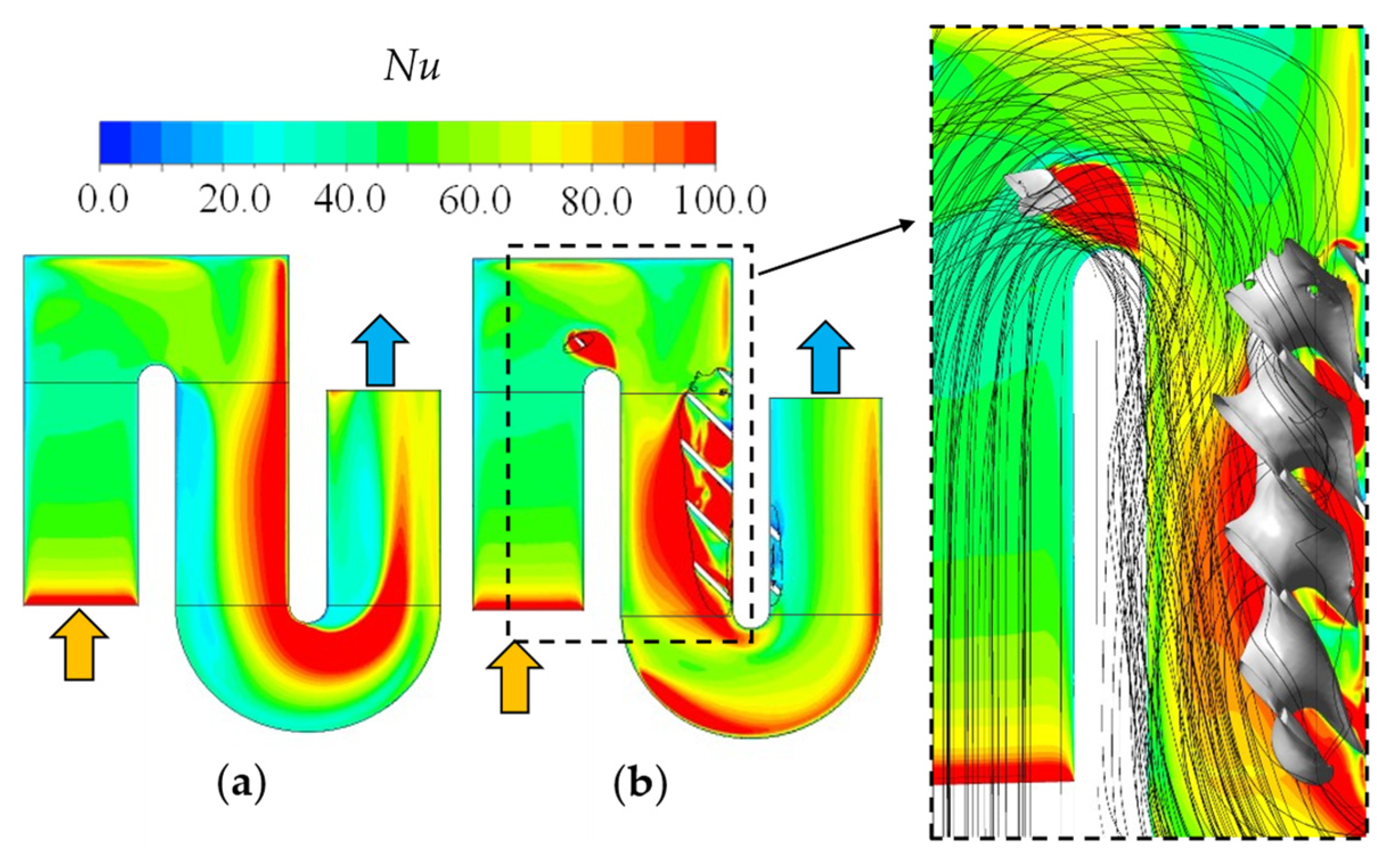
• The 3D optimized model with the diamond-TPMS structure significantly eliminates the recirculation flow and the low heat transfer regions at the second and third passages. This model also reduces the influence of Dean’s vortices but maintains high turbulence kinetic energy, leading to better uniform flow and heat transfer distributions.

Overall, the method in this work provides an advanced tool to manage the intermediate results in the conventional topology optimization of turbulent flow and heat transfer systems. Complex structures generated by this approach can be fabricated with additive manufacturing. Even though the present optimization models could be employed at a specific Reynolds number and heat input, this method can be applied to design cooling channels at higher Reynolds numbers and different cooling channel shapes, achieving higher thermal performance for gas turbine blades, heat sinks for high-power electronics, etc.

References

1. Yeranee, K.; Rao, Y. A Review of Recent Studies on Rotating Internal Cooling for Gas Turbine Blades. Chin. J. Aeronaut. 2021, 34, 85–113. [Google Scholar] [CrossRef]
2. Ekkad, S.; Singh, P. Detailed Heat Transfer Measurements for Rotating Turbulent Flows in Gas Turbine Systems. Energies 2021, 14, 39. [Google Scholar] [CrossRef]
3. Rao, Y.; Guo, Z.; Wang, D. Experimental and Numerical Study of Heat Transfer and Turbulent Flow Characteristics in Three-Short-Pass Serpentine Cooling Channels with Miniature W-Ribs. J. Heat Transfer. 2020, 142, 121901. [Google Scholar] [CrossRef]
4. Schüler, M.; Zehnder, F.; Weigand, B.; von Wolfersdorf, J.; Neumann, S. The Effect of Turning Vanes on Pressure Loss and Heat Transfer of a Ribbed Rectangular Two-Pass Internal Cooling Channel. J. Turbomach. 2011, 133, 021017. [Google Scholar] [CrossRef]
5. Guo, Z.; Rao, Y.; Li, Y.; Wang, W. Experimental and Numerical Investigation of Turbulent Flow Heat Transfer in a Serpentine Channel with Multiple Short Ribbed Passes and Turning Vanes. Int. J. Therm. Sci. 2021, 165, 106931. [Google Scholar] [CrossRef]
6. Lei, J.; Su, P.; Xie, G.; Lorenzini, G. The Effect of a Hub Turning Vane on Turbulent Flow and Heat Transfer in a Four-Pass Channel at High Rotation Numbers. Int. J. Heat Mass Transf. 2016, 92, 578–588. [Google Scholar] [CrossRef]
7. Sun, M.; Zhang, L.; Hu, C.; Zhao, J.; Tang, D.; Song, Y. Forced Convective Heat Transfer in Optimized Kelvin Cells to Enhance Overall Performance. Energy 2022, 242, 122995. [Google Scholar] [CrossRef]
8. Sigmund, O.; Maute, K. Topology Optimization Approaches: A Comparative Review. Struct. Multidiscip. Optim. 2013, 48, 1031–1055. [Google Scholar] [CrossRef]
9. Li, H.; Yamada, T.; Jolivet, P.; Kondoh, T.; Furuta, K.; Nishiwaki, S. Full-Scale 3D Structural Topology Optimization Using Adaptive Mesh Refinement Based on the Level-Set Method. Finite Elem. Anal. Des. 2021, 194, 103561. [Google Scholar] [CrossRef]
10. Li, H.; Kondoh, T.; Jolivet, P.; Furuta, K.; Yamada, T.; Zhu, B.; Zhang, H.; Izui, K.; Nishiwaki, S. Optimum Design and Thermal Modeling for 2D and 3D Natural Convection Problems Incorporating Level Set-Based Topology Optimization with Body-Fitted Mesh. Int. J. Numer. Methods Eng. 2022, 123, 1954–1990. [Google Scholar] [CrossRef]
11. Ghasemi, A.; Elham, A. A Novel Topology Optimization Approach for Flow Power Loss Minimization across Fin Arrays. Energies 2020, 13, 1987. [Google Scholar] [CrossRef]
12. Yeranee, K.; Rao, Y.; Yang, L.; Li, H. Enhanced Thermal Performance of a Pin-Fin Cooling Channel for Gas Turbine Blade by Density-Based Topology Optimization. Int. J. Therm. Sci. 2022, 181, 107783. [Google Scholar] [CrossRef]
13. Behrou, R.; Pizzolato, A.; Forner-Cuenca, A. Topology Optimization as a Powerful Tool to Design Advanced PEMFCs Flow Fields. Int. J. Heat Mass Transf. 2019, 135, 72–92. [Google Scholar] [CrossRef]
14. Zhang, B.; Gao, L. Topology Optimization of Convective Heat Transfer Problems for Non-Newtonian Fluids. Struct. Multidiscip. Optim. 2019, 60, 1821–1840. [Google Scholar] [CrossRef]
15. Alexandersen, J.; Andreasen, C. A Review of Topology Optimisation for Fluid-Based Problems. Fluids 2020, 5, 29. [Google Scholar] [CrossRef] [Green Version]
16. Manuel, M.C.E.; Lin, P.T. Heat Exchanger Design with Topology Optimization. In Heat Exchangers-Design, Experiment and Simulation; InTechOpen: London, UK, 2017. [Google Scholar]
17. Alexandersen, J.; Sigmund, O.; Aage, N. Large Scale Three-Dimensional Topology Optimisation of Heat Sinks Cooled by Natural Convection. Int. J. Heat Mass Transf. 2016, 100, 876–891. [Google Scholar] [CrossRef] [Green Version]
18. Dilgen, S.; Dilgen, C.; Fuhrman, D.; Sigmund, O.; Lazarov, B. Density Based Topology Optimization of Turbulent Flow Heat Transfer Systems. Struct. Multidiscip. Optim. 2018, 57, 1905–1918. [Google Scholar] [CrossRef] [Green Version]
19. Haertel, J.; Engelbrecht, K.; Lazarov, B.; Sigmund, O. Topology Optimization of a Pseudo 3D Thermofluid Heat Sink Model. Int. J. Heat Mass Transf. 2018, 121, 1073–1088. [Google Scholar] [CrossRef] [Green Version]
20. Li, H.; Ding, X.; Meng, F.; Jing, D.; Xiong, M. Optimal Design and Thermal Modelling for Liquid-Cooled Heat Sink Based on Multi-Objective Topology Optimization: An Experimental and Numerical Study. Int. J. Heat Mass Transf. 2019, 144, 118638. [Google Scholar] [CrossRef]
21. Li, H.; Ding, X.; Jing, D.; Xiong, M.; Meng, F. Experimental and Numerical Investigation of Liquid-Cooled Heat Sinks Designed by Topology Optimization. Int. J. Therm. Sci. 2019, 146, 106065. [Google Scholar] [CrossRef]
22. Zhang, B.; Zhu, J.; Gao, L. Topology Optimization Design of Nanofluid-Cooled Microchannel Heat Sink with Temperature-Dependent Fluid Properties. Appl. Therm. Eng. 2020, 176, 115354. [Google Scholar] [CrossRef]
23. Othmer, C. A Continuous Adjoint Formulation for the Computation of Topological and Surface Sensitivities of Ducted Flows. Int. J. Numer. Methods Fluids 2008, 58, 861–877. [Google Scholar] [CrossRef]
24. Ghosh, S.; Fernandez, E.; Kapat, J. Fluid-Thermal Topology Optimization of Gas Turbine Blade Internal Cooling Ducts. J. Mech. Des. 2021, 144, 051703. [Google Scholar] [CrossRef]
25. Dilgen, C.; Dilgen, S.; Fuhrman, D.; Sigmund, O.; Lazarov, B. Topology Optimization of Turbulent Flows. Comput. Methods Appl. Mech. Eng. 2018, 331, 363–393. [Google Scholar] [CrossRef] [Green Version]
26. Yoon, G. Topology Optimization Method with Finite Elements Based on the K-ε Turbulence Model. Comput. Methods Appl. Mech. Eng. 2020, 361, 15–18. [Google Scholar] [CrossRef]
27. Alkebsi, E.A.A.; Ameddah, H.; Outtas, T.; Almutawakel, A. Design of Graded Lattice Structures in Turbine Blades Using Topology Optimization. Int. J. Comput. Integr. Manuf. 2021, 34, 370–384. [Google Scholar] [CrossRef]
28. Wang, N.; Meenashisundaram, G.K.; Chang, S.; Fuh, J.Y.H.; Dheen, S.T.; Senthil Kumar, A. A Comparative Investigation on the Mechanical Properties and Cytotoxicity of Cubic, Octet, and TPMS Gyroid Structures Fabricated by Selective Laser Melting of Stainless Steel 316L. J. Mech. Behav. Biomed. Mater. 2022, 129, 105151. [Google Scholar] [CrossRef]
29. Kaur, I.; Singh, P. Flow and Thermal Transport Characteristics of Triply-Periodic Minimal Surface (TPMS)-Based Gyroid and Schwarz-P Cellular Materials. Numer. Heat Transf. Part A Appl. 2021, 79, 553–569. [Google Scholar] [CrossRef]
30. Pires, T.; Santos, J.; Ruben, R.B.; Gouveia, B.P.; Castro, A.P.G.; Fernandes, P.R. Numerical-Experimental Analysis of the Permeability-Porosity Relationship in Triply Periodic Minimal Surfaces Scaffolds. J. Biomech. 2021, 117, 110263. [Google Scholar] [CrossRef]
31. Kim, J.; Yoo, D.J. 3D Printed Compact Heat Exchangers with Mathematically Defined Core Structures. J. Comput. Des. Eng. 2020, 7, 527–550. [Google Scholar] [CrossRef]
32. Al-Ketan, O.; Ali, M.; Khalil, M.; Rowshan, R.; Khan, K.A.; Abu Al-Rub, R.K. Forced Convection Computational Fluid Dynamics Analysis of Architected and Three-Dimensional Printable Heat Sinks Based on Triply Periodic Minimal Surfaces. J. Therm. Sci. Eng. Appl. 2021, 13, 021010. [Google Scholar] [CrossRef]
33. Li, W.; Yu, G.; Yu, Z. Bioinspired Heat Exchangers Based on Triply Periodic Minimal Surfaces for Supercritical CO2 Cycles. Appl. Therm. Eng. 2020, 179, 115686. [Google Scholar] [CrossRef]
34. Borrvall, T.; Petersson, J. Topology Optimization of Fluids in Stokes Flow. Int. J. Numer. Methods Fluids 2003, 41, 77–107. [Google Scholar] [CrossRef]
35. Lazarov, B.; Sigmund, O. Filters in Topology Optimization Based on Helmholtz-Type Differential Equations. Int. J. Numer. Methods Eng. 2011, 86, 765–781. [Google Scholar] [CrossRef]
36. Celik, I.B.; Ghia, U.; Roache, P.J.; Freitas, C.J.; Coleman, H.; Raad, P.E. Procedure for Estimation and Reporting of Uncertainty Due to Discretization in CFD Applications. J. Fluids Eng. Trans. ASME 2008, 130, 0780011–0780014. [Google Scholar] [CrossRef] [Green Version]
37. Winterton, R.H.S. Where Did the Dittus and Boelter Equation Come From? Int. J. Heat Mass Transf. 1998, 41, 809–810. [Google Scholar] [CrossRef]
Figure 1. Numerical model of a three-short-pass serpentine channel: (a) full 3D model; (b) 2D simplified design from the 3D model.
Energies 15 08924 g001
Figure 2. Overview of the procedures in this study.
Energies 15 08924 g002
Figure 3. Flow chart of the topology optimization process.
Energies 15 08924 g003
Figure 4. A single unit cell of (a) diamond-sheet structure; (b) gyroid-sheet structure for fulfilling the optimal results in this study.
Energies 15 08924 g004
Figure 5. (a) The mesh system for 2D model validation; (b) mesh system in the 3D model.
Energies 15 08924 g005
Figure 6. Comparison of the average values of the state variables between 2D and 3D at Re = 10,000: (a) pressure values; (b) velocity magnitudes; (c) temperature values.
Energies 15 08924 g006aEnergies 15 08924 g006b
Figure 7. The optimized 2D model with intermediate results.
Energies 15 08924 g007
Figure 8. (a) 3D optimal solution including intermediate results; (b) topology optimization model infilled with lattice structures.
Energies 15 08924 g008
Figure 9. Models for comparison: (a) optimized model extracted with density filtering of 0.5 (TO model); (b) optimized model infilled with diamond-sheet structure (TO model with diamond-TPMS); (c) optimized model infilled with diamond-sheet structure (TO model with gyroid-TPMS).
Energies 15 08924 g009
Figure 10. An example of mesh systems for the 3D models.
Energies 15 08924 g010
Figure 11. The spanwise-averaged temperature and grid convergence index on the surface of the conventional serpentine channel at Re = 10,000.
Energies 15 08924 g011
Figure 12. Comparisons of globally averaged Nusselt number in each pass for different turbulence models at Re = 10,000.
Energies 15 08924 g012
Figure 13. Comparisons of relative pressure coefficient for all serpentine channels at Re = 10,000.
Energies 15 08924 g013
Figure 14. Friction factors for all serpentine channels at Re = 10000.
Energies 15 08924 g014
Figure 15. Globally averaged Nusselt numbers for all serpentine channels at Re = 10,000.
Energies 15 08924 g015
Figure 16. Total Nusselt numbers for all serpentine channels at Re = 10,000.
Energies 15 08924 g016
Figure 17. Heat transfer enhancements for all serpentine models at Re = 10,000: (a) globally averaged Nusselt number ratio; (b) total Nusselt number ratio.
Energies 15 08924 g017
Figure 18. Thermal performances for all serpentine models at Re = 10,000.
Energies 15 08924 g018
Figure 19. Temperature uniformity on the surface for all serpentine models at Re = 10,000.
Energies 15 08924 g019
Figure 20. Velocity distributions and streamlines in the middle section of the serpentine channel: (a) baseline model; (b) TO model with diamond-TPMS structure.
Energies 15 08924 g020
Figure 21. Pressure distributions in the middle section of the serpentine channel: (a) baseline model; (b) TO model with diamond-TPMS structure.
Energies 15 08924 g021
Figure 22. Local dimensionless turbulent kinetic energy and velocity streamline on the cross-sections in the multipass channel: (a) baseline model; (b) TO model with diamond-TPMS structure.
Energies 15 08924 g022
Figure 23. Nusselt number contours of the serpentine channel: (a) baseline model; (b) TO model with diamond-TPMS structure.
Energies 15 08924 g023