Article

Forecasting Short-Term Electricity Load Using Validated Ensemble Learning

1
Sirindhorn International Institute of Technology, Thammasat University, Pathum Thani 12000, Thailand
2
Department of Electrical and Information Engineering, Faculty of Engineering, University of Ruhuna, Galle 80000, Sri Lanka
*
Author to whom correspondence should be addressed.
Energies 2022, 15(22), 8567; https://doi.org/10.3390/en15228567
Submission received: 6 October 2022 / Revised: 9 November 2022 / Accepted: 9 November 2022 / Published: 16 November 2022
(This article belongs to the Topic Short-Term Load Forecasting)

Abstract

:
As short-term load forecasting is essential for the day-to-day operation planning of power systems, we built an ensemble learning model to perform such forecasting for Thai data. The proposed model uses voting regression (VR), producing forecasts with weighted averages of forecasts from five individual models: three parametric multiple linear regressors and two non-parametric machine-learning models. The regressors are linear regression models with gradient-descent (LR), ordinary least-squares (OLS) estimators, and generalized least-squares auto-regression (GLSAR) models. In contrast, the machine-learning models are decision trees (DT) and random forests (RF). To select the best model variables and hyper-parameters, we used cross-validation (CV) performance instead of the test data performance, which yielded overly good test performance. We compared various validation schemes and found that the Blocked-CV scheme gives the validation error closest to the test error. Using Blocked-CV, the test results show that the VR model outperforms all its individual predictors.

Graphical Abstract

1. Introduction

The increased energy demand due to the rise in the population over the past few decades has been an eye-opener for the efficient use of energy all over the world. One of the critical objectives of energy forecasting is to allocate a sufficient and efficient energy supply to cater for the future demand. Many countries seek alternative energy resources to balance supply and demand [1]. Therefore, forecasting the required demand at least for a 1 day ahead has become a popular theme among energy providers to maintain that equilibrium.
Forecasting is divided into three subsections according to the prediction horizon: short-term load forecasting (STLF), medium-term load forecasting (MTLF), and long-term load forecasting (LTLF) [2]. Each plays a different role in the power system, benefiting supply and demand-side management. Accurate forecasting of a country’s short-term electric energy demand is the key to making day-to-day decisions on hourly/day-ahead demand compared to the medium-term and long-term forecasts. Forecasting the electric energy demand is carried out by developing models using historical data, and many factors, such as climate conditions, calendar parameters, and some seasonal features [3]. Since Thailand is a tropical country, its electric demand is heavily influenced by climate and weather conditions, along with many public, religious, and long holidays. The limited research on Thai data found in the literature, which will be further elaborated in Section 2, suggests that the accuracy of short-term forecasting can be further improved with a better selection of features and using appropriate models.
Machine learning (ML) plays a leading role when predicting electricity demand compared to classical methods, such as statistical time series analysis and smoothing techniques. They have become popular among developers because of their convenient computer implementation and ability to produce both linear and nonlinear, parametric/non-parametric models suitable for the nature of the data. If sufficient historical data are available to train a model, supervised learning is used. Adequate feature engineering must also tackle a time series’s seasonality, trend, and possible irregularities. Unarguably, there are many ML models already developed to forecast demand. For example, in [4], the authors applied regression and neural network (NN) to their dataset as ML methods. However, the prediction accuracy of such models is still questionable, since the model’s variables and hyper-parameters were selected from the test performance on the test data.
Model evaluation is crucial in ML before launching the model in practice. Developers use various validation techniques to evaluate a model’s performance to ensure that the model generalizes well for unseen data. After time series analysis, the most preferred technique is cross-validation (CV). However, the use of CV in the context of time series is questionable because of the potential non-stationarity and the serial correlation of data [5]. However, as proposed in [5], cross-validation can be used in time series if the series is stationary. Since it is hard to find studies on Thai electricity load data that have used validation techniques to select the best models, model variables, and parameters, we used cross-validation in this work. However, to use it, we needed to show that our data are stationary.
Many available supervised ML predictors are standalone learners. The accuracy of the predictions might be low when considered individually. However, the forecasts from multiple independent forecasters can be combined to form a better forecaster [6]. Regarding Thai data in our context, the use of EL is lacking in the literature. Therefore, this research focused on developing a cross-validated EL model to forecast the short-term electricity load in Thailand.

Main Contributions

The main contributions of this paper are summarized as follows:
  • We extended our previous work in [4] using the same dataset and data grouping approach to use cross-validation. In our previous work, we used the test error to check the model’s performance, which might have resulted in overly good test performance due to over-fitting the test data.
  • We considered linear regression models with decision tree and random forest methods. We combined the forecasting models via a simple fixed-weight ensemble learning with the weights selected manually to improve the forecasting performance. Although simple, this ensemble learner outperforms all other individual forecasting models.
  • We show via the augmented Dickey–Fuller (ADF) test that our data are stationary and have high confidence levels. This means we can use the cross-validation schemes for our time-series data.
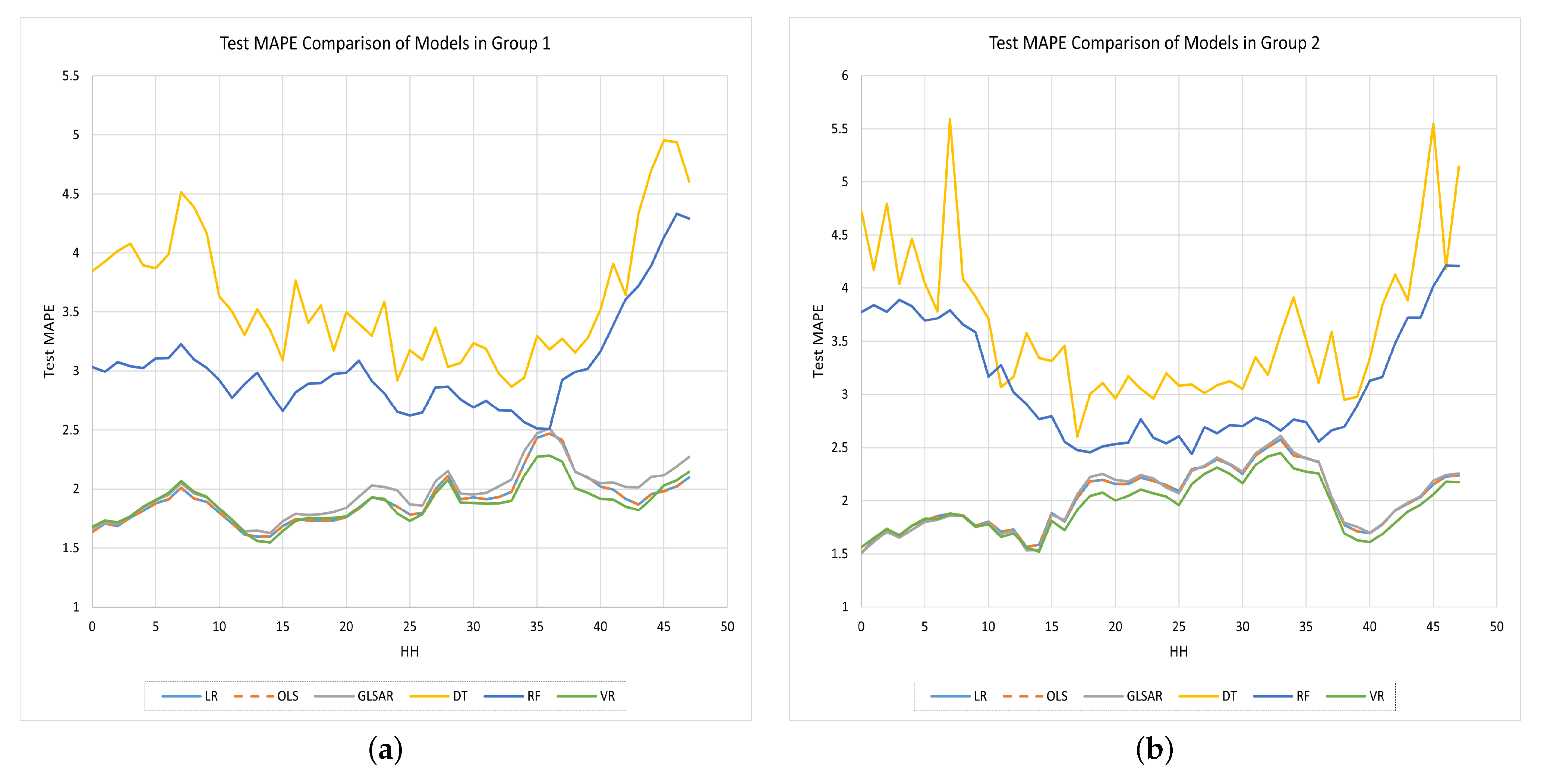
  • For each forecasting model, we evaluated the performances of three validation schemes and found that most of the time, the Blocked-CV scheme gives the best performance, and these results are also the closest to those of the ensemble model.
  • Using this validation scheme, the test results show that the ensemble learning model outperforms all its individual predictors.
The remainder of the paper is structured as follows. Section 2 presents a detailed discussion of the related works. Section 3 presents the methods, including the data preparation, selection of the prediction horizon, and overall model design procedure, which includes the details of all the estimators used and their model evaluation schemes. Section 4 presents the results, extensively comparing the forecasting accuracies of the individual predictors based on the validation and the test errors. Finally, Section 5 concludes on the findings and highlights some limitations and possible future directions.

2. Related Works

2.1. Categories of Load Forecasting Based on the Prediction Horizon

As previously mentioned, STLF, MTLF, and LTLF are the three main categories of load forecasting based on different prediction horizons [2]. Some researchers introduce another category called very short-term load forecasting (VSTLF), which runs from only a few minutes to hours [7]. A comparison of forecasting in different time scales and examples of their applications are given in Table 1.
In common, there are several advantages of forecasting the electric energy demand, both economic and environmental [12]. One of the most straightforward benefits, if predictions are accurate, is that there will be no unintentional over-generation of energy so that it would reduce the costs associated with any possible wastage [13]. The same would reduce environmental impacts, such as the emission of CO 2 and global warming. On the other hand, any underestimation of demand can result in severe power outages, risking the power system’s stability, security, and reliability.
The focus of this research is on SLTF, whose horizon usually runs from hours to a week. Energy providers use it to plan their day-to-day operations. Effective forecasting helps them to decide on when and which power plants to operate and/or shut down to cater to the required demand. That process is called unit commitment (UC), which ensures the optimum utilization of resources. Furthermore, the energy providers also aim to meet the required demand at a minimum cost. That is called economic dispatch (ED), which is beneficial not only for the providers but also for the consumers. ED and UC are considered direct benefits of STLF [2].
The works on SLTF for Thailand seem to have appeared only recently. Using the same dataset that we used in this work (i.e., the data from the Electricity Generating Authority of Thailand (EGAT) from 2009 to 2013), several works have been published [4,8,9,14,15,16]. The STLF model implemented in [4] implemented 1-day ahead forecasting by setting the prediction horizon as 10 to 34 h.

2.2. Factors Affecting the Electric Energy Demand

Due to the auto-regressive and periodic nature of electricity consumption, the historical or lagged load is a crucial factor to determine the electricity load. Huang and Shih [17] developed a univariate auto-regressive moving average (ARMA) model capable of handling both Gaussian and non-Gaussian processes. However, consideration of other factors which affect the electric energy demand is essential. As explained previously, the demand is also affected by weather/climate conditions, calendar parameters, and seasonal features. A time-varying periodic spline model with temperature as the exogenous variable was used in [18] and achieved the mean absolute percentage error (MAPE) value of about three. Using the same dataset for this study, Chapagain and Kittipiyakul [8] developed two MLR models and showed that the model with added temperature variables resulted in an at least 20% accuracy improvement.
In [4], calendar parameters such as year, month, day of the week, and hour; and seasonal features such as holidays and special days, were taken into account as driving factors for the demand and used, along with other essential factors, to develop many predictive models. In general, these factors are called deterministic variables. The demand on weekdays has significantly different patterns compared to the demand on weekends [19]. Specifically, weekday demand is considerably higher and more stable compared to weekend demand due to the presence of industrial sector operations on weekdays. Holidays, whether on weekdays or weekends, see much lower demand. Therefore, we needed to assign dummy variables to represent the seven days of the week as weekdays, weekends, and holidays so that the different day types would be clearly specified.
Since we used the same dataset as in [4], we used a similar set of dummy variables to represent the deterministic variables. Holidays/special days, such as bridging working days between weekends and a major holiday or days before and after major holidays, also affect the electric demand, and ignorance of their effects in a model can result in a severe dip in accuracy. Non-stationarity in the data series due to special days can be overcome by either introducing dummy variables or creating separate models for each hour or half-hour. With the same dataset we used, Chapagain et al. [4] selected both options and obtained better results. Since it is a Thai electric demand dataset, the special day factors considered were Newyear, Songkran, etc. To make the predictions more accurate, they introduced a series of dummy variables representing different holiday types and the days before/after special days, as in [20].
Introducing interaction variables helps to increase forecasting accuracy. For example, since the weekday demand is more sensitive to the weather parameters compared to the weekend demand, implementing interaction terms between the demand and the meteorological parameters, such as the temperature, after separating the weekdays and weekends, has resulted in a significant accuracy improvement [21]. Furthermore, since historical demand is used to predict the next day’s demand, there is a possibility of an error in predicting the days around the margins between weekdays and weekends, since the weekend demands are significantly less than on weekdays. Therefore, interaction terms between the day-of-the-week dummy variables and the lagged load up to two days were introduced in [4]. They also included interaction terms between the day-of-week/month dummy variables and temperature to improve accuracy further.

2.3. Importance of Grouping the Dataset

Grouping a dataset into categories with similar demand patterns helps to improve the accuracy of predictions. For example, working days/weekdays, weekends, and holidays have their own demand patterns. Using the same EGAT dataset and grouping, Chapagain et al. [4] built separate models and achieved improved results compared to having a single model trained with the entire dataset. They achieved 1.81%, 1.74%, and 16.63% MAPE accuracy for weekdays, weekends, and holidays, respectively. Since the holiday’s prediction accuracy became worst due to limited observational data, they went with a model trained with the entire dataset to predict the holiday demand and achieved an overall MAPE of 2.95%. A similar kind of grouping was carried out in [3] but using an energy dataset from a cold region in Japan. They achieved 0.9%, 1.81%, 2.51%, and 1.72% MAPE for weekdays, weekends, holidays, and overall demand, respectively.
Another effective two-fold grouping was also found in the literature as working days and holidays [22]. Srinivasan et al. [23] considered holiday demand to resemble the demand on Sundays and divided the dataset into working days, holidays and Sundays, and Saturdays. They achieved impressive performance with 1% MAPE for all three categories. Su and Chawalit [24], followed by [25], introduced seven groups of training data—Monday, Tuesday, etc.—considering the days of the week. The authors of the latter research eliminated the holiday and bridge-holiday effects by replacing them with the weighted average load of the same day of the week from the previous two weeks.

2.4. Predictive Methods

Methods used to build forecasting models can be classified into two main categories: classical methods and machine-learning methods. A few examples of classical methods used in the literature are statistical time series analysis; and the ARMA model and its extensions, such as auto-regressive integrated moving average (ARIMA), seasonal auto-regressive integrated moving average (SARIMA), auto-regressive moving average with exogenous variable (ARMAX), and regression methods. However, their applications are limited to supporting only linear problems or limited forms of nonlinearity. A comparison between linear and nonlinear models for forecasting short-term electricity demand in Czech was performed in [22]. They concluded that forecasting the Czech electricity demand is almost a linear problem. The selected linear ARIMA model outperformed the nonlinear NN model in univariate and multivariate cases. Taylor et al. [26] compared six different univariate short-term demand forecasting models with an hourly dataset in Brazil and a half-hourly dataset in England. The double seasonal exponential smoothing model and the ARMA model outperformed all other models in the accuracy of the predictions.
An ARMAX model was developed using the same dataset we used for our study. By including temperature as the exogenous variable and another set of dummy variables, the short-term electric demand in Thailand was forecast [4]. The estimation methods used in the ARMAX model were MLR:OLS for non-serially correlated error cases and GLSAR for serially correlated error cases. These two estimation methods of the ARMAX model were then compared with a NN, and the results showed that the ARMAX model outperformed the NN. Another study was conducted in [27]. Three different ARMA(2,6) models were built to predict short-term electricity demand in Hokkaido, Japan. One of the models included some meteorological parameters—temperature, wind speed, relative humidity, solar irradiation, etc.—as the exogenous variables to make it an ARMAX model. The results showed that the ARMAX model had a performance improvement of at least 0.015% compared to the other two models.
Machine learning is now more often used for energy forecasting applications compared to classical methods. The main reason for this is their applicability in linear and nonlinear problems so that the seasonality issues can be quickly taken care of. The models developed in ML also can be parametric or non-parametric. ML models such as artificial neural networks (ANN), fuzzy logic, and support vector machines (SVM) are good examples in recent literature. Three machine learning models were developed in [28]—SVM, nonlinear auto-regressive (NAR) recurrent ANN, and long short-term memory (LSTM) ANN—to do multi-step ahead forecasting in residential microgrids. Those ML models outperformed an ARMA model. One of the problems of ML approaches such as SVM and ANN is their vulnerability to getting stuck at a local optimum during the training. Furthermore, an improved version of an LSTM model with the empirical wavelet transform (EWT) developed in [29] outperformed several benchmark ML models, resulting in MAPE values below 6% for three real-life cases.
ML models used for STLF with Thai data are limited in the literature. For example, a combined particle swarm optimization (PSO) algorithm that used the ANN technique to forecast the short-term electric demand in Thailand was developed in [15]. They achieved the overall training MAPE accuracy of 3.44%. Furthermore, they extended their work by introducing a hybrid PSO with a genetic algorithm (GA) and improved their accuracy to 2.86% [25]. Su and Chawalit [24] used more recent data than us to develop a deep neural network (DNN), SVM, and NN to forecast the short-term energy demand in Thailand. They found that the best test MAPE result among all the considered methods was 4.2% using one of the DNN methods.
Not only in electric energy management but in many other fields is time-series forecasting being used. A classical example is electricity price forecasting, as in [30,31]. They have used functional auto-regressive (FAR) models to optimally forecast the short-term electricity prices and demand in different electricity markets. Furthermore, they have proved that their component (deterministic and stochastic) estimation technique is highly effective at forecasting electricity prices based on the short-term [32] and the medium-term demand [33].

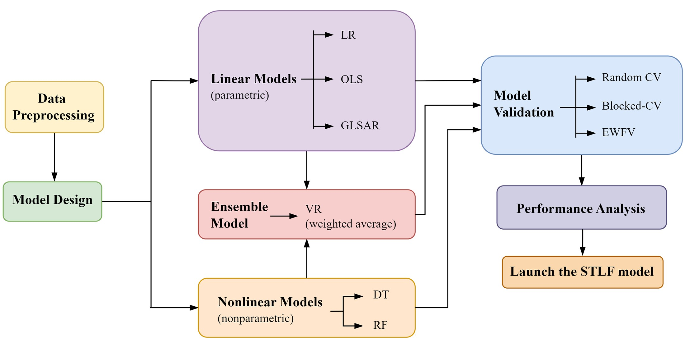
2.5. Model Validation Techniques

There is an apparent scarcity of time series research that uses model validation schemes to evaluate models and select the best hyper-parameters. The main reason for that gap is that many developers believe validation is meaningless in time series data, since they are prone to being serially correlated [5]. For independent and identically distributed (i.i.d) data series, CV is used extensively to randomly divide the whole training dataset into several validation sets for evaluation. Nevertheless, with time-series data, developers omit that, since the random selections could create holes in the dataset destroying the auto-correlative nature and could easily leak future information to the model [34].
Recently, several works [5,34,35] have started to look at when CV can be applied to time series and which CV techniques are most appropriate. Validation is divided into two categories: CV schemes and forward validation (FV) schemes. Each of them has its extensions. Since Random CV causes problems with time series data, Nielsen [34] suggested two FV schemes, EWFW and rolling window forward validation (RWFV), for model validation. However, they used the whole dataset, including the test set, to combine the full training, validation, and testing. In addition, Schnaubelt [35] compared eight different validation schemes with three different ML models—LR, RF, and NN—including both CV and FV extensions on non-stationary time-series data produced by a synthetic data-generating process (DGP). Six validation schemes were 5-fold, and the other two were derivations of a test-set-evaluation-like approach called last-block validation (LBV). The author compared the validation error of each scheme with the test error and selected the scheme, which yielded the minimum difference between them. The author concluded that the FV schemes perform well when the perturbation strength of the stationarity gets higher. However, with a closer look at the results, the author suggested that CV and FV schemes perform similarly for small perturbation strengths and prefer LBV if the perturbation strength is very high.
Validity of k-fold CV in time series forecasting under a few conditions was proved in [5]. The conditions allowing the use of k-fold CV are:
1.
the AR process should be stationary,
2.
the model should be purely auto-regressive,
3.
the model should be nonlinear and non-parametric (preferably an ML model), and
4.
the fitted model should have uncorrelated errors/residuals.
They compared three different CV schemes: 5-fold CV, 5-fold non-dependent CV (nonDepCV), and leave-one-out CV (LOOCV), with an LBV-like approach, called out-of-sample (OOS) evaluation, in a linear and a nonlinear model. They used standard multi-layer perceptron (MLP) NN as the nonlinear model. The results showed that the CV schemes outperformed the OOS evaluation. They applied the Ljung box test to check the serial correlation of residuals. They used an AR(5) model as the linear model, and the results reflected the same. The authors indirectly suggested that if the series is stationary and the model is linear, then CV can be applied without any problems.
It is not easy to find research on Thai electricity load data that has used validation techniques to evaluate the forecasting models. The ARMAX model used in [4] followed a similar RWFV-like training and testing pattern, as explained in [34], but real validation of the model could not be seen there.

2.6. Ensemble Methods
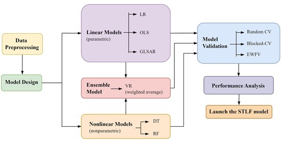
The method of producing a robust model by combining a diverse set of individual learners is called ensemble learning (EL) [6]. The simplest form of an ensemble in classification is the voting classifier (VC) which aggregates the predictions of each model. A similar form called the voting regressor (VR) is available for regression tasks. It takes the majority voted class in the case of classification, but it is the simple average or the weighted average for regression. In this work, we developed a voting regressor with weighted averaging as our EL model.
In addition to the voting EL models, there are three main methods of building more complex EL models: bagging, boosting, and stacking [6]. Unlike VR, bagging uses a single base estimator trained with different random samples of the entire dataset. An ensemble of multiple DTs called RF uses the bagging method to train its model. Boosting is quite different, as it can use different learners and tries to evolve by correcting the errors of each predecessor. In contrast, stacking uses at least two stages of predictions. The first stage can have multiple learners while using all of their predictions to train the second stage, and so on.
Many researchers recently adopted the ensemble approach due to the proven accuracy improvement in the predictions. A survey of load forecasting models for power system management was conducted [2]. They included information about linear models such as MLR, exponential smoothing, and nonlinear models such as NN. Finally, they preferred the ensemble approach to get an optimum forecast by combining those multiple predictive models with a probabilistic nature. Divina et al. [12] developed a stacking ensemble-learning model to forecast short-term electric energy demand using a dataset in Spain collected over nine years. Their model included two stages. In the first stage, they used three regression-based machine-learning models: evolutionary decision tree (EvTree), RF, and NN. Their predictions were then input to the second stage generalized boosted model (GBM) to have the ultimate predictions, which were finally found to be more accurate than all three first stage models.
EL methods have also been used to forecast electric demand in Thailand, particularly for medium-term forecasting. For example, using Thai electric peak demand data from 2002 to 2017, reference [10] developed and compared several medium-term forecasting models: ANN, SVM, deep belief network (DBN), and their ensembles. The EL models used a simple averaging method similar to VR to aggregate the predictions. The results showed that the ensemble model built by combining the ANN and DBN models outperformed other models for 1-month-ahead forecasting with a MAPE accuracy of 1.44%.
EL is used in other fields, such as electricity price forecasting, as in [36]. They modeled their stochastic component using an ensemble of ARMA, neural network auto-regressive (NNAR), RF, support vector regression (SVR), and GBM. The results suggest that the proposed EL method efficiently predicts electricity prices in the Italian electricity market (IPEX).
A summary of recently published state-of-the-art related work that used our full dataset or a part of the dataset to perform SLTF in Thailand is given in Table 2.

3. Methods

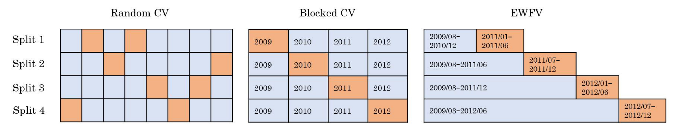
3.1. Data Preparation

The dataset used to train and test the models throughout this study was provided by EGAT, the leading player in the Thai energy market possessing almost 50% of the generation and 100% of transmission system. EGAT divides the country into five regions and keeps recordings of the electric loads separately. The central region, MCC, which includes Bangkok and nearby provinces with the highest electricity demand, is the focus of this research. The dataset includes 84,816 instances of half-hourly electricity load (in MW) and the corresponding half-hourly temperature measurements (in °C) for almost about five years (from 1 March 2009 to 31 December 2013). This dataset has been used in many studies to develop different forecasting models in recent years [4,8,14,16]. The final dataset provided for this study was a preprocessed version of [4], after filling in some missing load values and some temperature adjustments. The preprocessed data also include deterministic, meteorological, historical load, and interaction terms.
As in [4], the half-hourly data from 29 March 2009 to 31 December 2012 were selected as the training set, which included almost four years (65,952 instances); we kept aside the year 2013 for the test data (17,520 instances). We started training from 29 March 2009, since we used a 28-day lag load as one of the features in our models.
As grouping the dataset proved to simplify modeling and showed a significant accuracy improvement in the literature, as discussed in Section 2.3, the dataset was divided into four different groups, as illustrated in Figure 1, similarly to [4].
Since the dataset included half-hourly (HH) data, each group was further divided into N = 48 subsets (of similar half-hours). Therefore, the training and test instances for each HH in each group were as follows.
Group 1: train = 896, test = 239
Group 2: train = 336, test = 87
Group 3: train = 142, test = 39
Group 4: train = 1374, test = 365
The corresponding training sets were used to train and validate the models. The model selection in our study was based on the validation error. We did not use a rolling window approach like in [4] to train and test the models. Therefore, the test sets were only used to check the performances of the models trained with all the training data.

3.2. Prediction Horizon

Since for each working day, EGAT collects load data up to 2 pm and makes forecasts for the next day’s demand, the HH forecasts are generally 10 to 34 h ahead. Our study is also limited to predicting 10 to 34 leading hours of the next day, considering the data up to 2 pm are available for the current day. However, the “next day” has quite a different meaning here, since the dataset is divided into groups. For example, it is 1-day ahead forecasting in Group 4. However, in the case of Group 2, where it uses only weekends to train the model, the next day for Saturdays is Sunday (1-day ahead), but for Sundays, it is the following Saturday (6-days ahead). Similarly, Groups 1 and 3 also have their unique interpretations for the “next day”.

3.3. Model Design

The general workflow of this work is shown in Figure 2. It had five major steps: data preparation, model design, linear/nonlinear/ensemble estimation, model evaluation, and performance analysis. Details of the data preparation have already been discussed in Section 3.1.
The overall model consists of five different individual predictors and their ensemble. Those individual predictors are a set of classical and ML regression-based methods. Classical methods include three MLR-based parametric ARMAX models, which use LR, OLS, and GLSAR as estimators; and ML methods include two nonlinear nonparametric estimators: DT and RF. The LR and OLS models are generally used for cases assuming uncorrelated errors, and the GLSAR is for correlated errors. DT and RF are selected due to their well-known adaptability to nonlinear nature of data.
For each group, these linear and nonlinear models were the training and test data as explained in Section 3.1. They commonly used the lag loads (1-day, 7-day, 14-day, 21-day, and 28-day), temperature as the exogenous variable, and some other deterministic and interaction variables to tackle the seasonal effects. Corresponding feature identifications for each group are presented in Appendix A.1. Since we did not use the rolling window approach [32] to estimate the models, the parameters remained constant for a given half-hourly model in a given group, irrespective of the day we predicted. Furthermore, a major difference experienced between linear and nonlinear models was that the model parameters of the MLR process could be known for the linear models but not the nonlinear models.

3.3.1. Parametric Models

The MLR-based ARMAX models used in this study were parametric models which used a fixed number of parameters/features. Therefore, we built an equation representing the relationship between the target variable (load) and the features. The features included deterministic variables, temperature, lag loads, and interaction terms. Since each group’s datasets was divided into 48 subsets, each model included 48 individual equations to perform a 1-day forecast. The demand at day d and half-hour h was modeled as
D h , d = i = 1 n α i · ( D t h , d ) i + i = 1 m β i · ( T m p h , d ) i + i = 1 p θ i · ( L L h , d ) i + i = 1 q γ i · ( I t h , d ) i + μ h , d
where D t h , d , T m p h , d , L L h , d , and I t h , d are groups of deterministic, temperature, lag loads, and interaction terms, respectively. Similarly, α , β , θ , and γ are groups of their corresponding coefficients. The error term μ h , d N ( 0 , ) is vital to address, since it tends to be serially correlated with errors in previous days. Depending on the properties of ∑, the model is classified as [4]:
1.
OLS/LR: for i.i.d errors = I
2.
GLSAR: for AR(p) errors = ( ρ )
Therefore, we used OLS and LR models with the assumption of uncorrelated errors and the GLSAR with AR(1) structure for the correlated errors in our study. The mathematical forms for OLS and LR models were quite similar and followed the exact representation of the OLS model given in [4]. However, during the parameter estimation process, OLS used the matrix inversion to minimize the loss function, and LR used the iterative gradient-descent algorithm. GLSAR also used the same mathematical form given in [4] with correlated errors, but we selected the AR(1) structure. The Durbin–Watson (DW) test on the errors/residuals of the models was conducted to check for any serial correlation. Its test statistic usually ranges from 0 to 4. The values between 1.5 and 2.5 suggest no significant serial correlation of errors.

3.3.2. Nonparametric Models

The DT and the RF were the nonlinear nonparametric models used in this study. Compared to parametric models, DT and RF do not have a fixed set of features in a predetermined form but can be adjusted according to the information derived from the data. Therefore, it was impossible to formulate a relationship between the features and the target variable as we did with the parametric models.
DT is a robust ML algorithm that forms a tree-like structure to predict the target variable based on the decision rules induced by the features [6]. Each internal node, branch, and leaf node of the tree consist of a test conducted on a feature, the outcome of the test, and the final decision which predicts the target variable, respectively. Usually, DT models are prone to over-fitting, since they have high flexibility. The over-fitting could be overcome by fine-tuning their hyper-parameters. By comparing the CV MAPE of a DT model with different random sets of hyper-parameters, as shown in Table A3 of Appendix A.2, we selected a good hyper-parameter combination to proceed (random_state = 42, max_depth = None, min_samples_split = 10, min_samples_leaf = 5, max_features = None, max_leaf_nodes = None, etc.).
RF is an ensemble of several DTs trained on random subsets of instances and the dataset’s features. It uses averaging to improve the accuracy of the prediction and controls the over-fitting [6]. It usually uses bootstrap sampling with the max_samples set to the size of the train set. The hyper-parameters for the RF model were also selected in a similar approach to DT (n_jobs = −1, random_state = 42, n_estimators = 100, max_depth = None, min_samples_split = 4, min_samples_leaf = 2, max_features = 1.0, etc.), as shown in Table A4 of Appendix A.2. One issue is the time it takes to train several DTs, which was compensated for by allocating all available cores on the machine.

3.3.3. Ensemble Model

The EL model was developed by optimally combining the five aforementioned individual predictors’ outputs. This is a VR model which uses the weighted-averaging method to predict the demand. For simplicity, the corresponding weights ( w 1 , , w n ) were realized by a trial-and-error method giving higher weights for individual models with higher accuracies. The predicted demand using the VR model at day d and half-hour h can be modeled as
( D ^ h , d ) V R = i = 1 n w i . ( D ^ h , d ) i ,
where n and ( D ^ h , d ) i represent the number of individual predictors (n = 5 in our case) and the predicted demand with the ith individual model at day d and half-hour h, respectively. The method of identifying the best set of weights for the VR model is presented in Appendix A.3. It is expected that VR has the best prediction accuracy compared to all other individual models. Although there are various performance metrics, we use the mean absolute percentage error (MAPE), defined as
M A P E = 1 N | D | k = 1 N α D D h , d D ^ h , d D h , d × 100 % ,
where N = 48; D represents the set of test days; and D h , d and D ^ h , d represent the actual demand and predicted demand, respectively, at day d and half-hour h [4].

3.3.4. Model Evaluation

Our work used the validation error to select the best model, model features, and model parameters. Validation was conducted with the training dataset, which provided an additional measure of the model’s accuracy before testing with unseen data. We used three different 4-fold validation schemes, Random CV, Blocked-CV, and EWFV, on the training set (2009–2012). They were set to 4-fold validation, since the training set spanned four years. Figure 3 illustrates the three validation schemes.
If the ith data split of a validation scheme x has the validation error of e i , x , the overall validation error ( E v , x ) for scheme x is given as the average across all splits:
E v , x = 1 s i = 1 s e i , x ,
where s represents the number of splits (s = 4 in our case).
We used the standard k-fold CV as the Random CV here with k = 4. The issue with this scheme for time series data is evident, since it randomly selects the validation folds without considering any serial correlations/dependencies of the data. Furthermore, this randomness could cause a validation fold to become a weaker representative of the full-time series dataset. However, it is still applicable if the time series is found to be almost stationary [35], and that is one primary reason for us to find the stationarity of the data series at the beginning before putting them into the models.
Blocked-CV seems the most attractive scheme, since it uses each year from 2009 to 2012 as its four validation folds, making each fold uniform and a clear representation of the entire dataset. For example, if any annual seasonality persists on the entire dataset, a one-year fold can represent that. However, the Blocked-CV still has a dependency issue, but at a lower level compared to Random CV, since the selection of the validation fold is no longer random, and the validation fold for each split breaks precisely at the beginning/end of the year.
The previous two schemes are categorized as CV schemes, and the last, EWFV, as an FV scheme. The main difference between CV and FV is that the latter never uses future data to predict the past data so that it can adapt well to deal with possible non-stationarity in time series data [35]. This difference also benefits validation with time series data, providing a minimum dependency issue. One major characteristic of EWFV is that it uses validation folds with a fixed size while increasing the size of the training folds with every split. For example, we used data from March 2009 to December 2010 to create the training fold of the first split and selected only the following six months (from January 2011 to June 2011) as the validation fold. Therefore, we had the disadvantage of inefficient data usage, since the initial splits did not cover all available data.

3.3.5. Performance Analysis

As stated in Equation (3), the performance index used to measure the accuracy of the predictions in this study was the MAPE value. The usual practice is to use the test accuracy (or the test MAPE value) to decide the final model. However, the overall model developed here is capable of determining all the training, validation (for all three schemes discussed in Section 3.3.4), and test MAPE values denoted by E t r a i n , E v , x , and E t e s t , respectively, for each model, including the EL model in each group.
For each model in each group, the validation scheme with the minimum difference between the E v , x and E t e s t values in the majority was chosen as the final validation scheme. Furthermore, the model with the minimum validation MAPE under that chosen validation scheme denoted by E v , x * in each group was selected as the final model. It was expected that the minimum validation error E v , x would lead the final model to reflect the minimum test error E t e s t too, which is proved with experimental results in Section 4.

4. Results and Discussion

We first show the results of the stationarity test of our data to show that it is stationary and has high confidence levels, and hence validation schemes can be applied. Then, we performed the training and validation of different models. We then evaluated the models with their best hyper-parameters and/or features on the test data to compare the test performance with the validation performance.

4.1. Checking for the Stationarity of Time-Series Data

It is required to analyze the given time series dataset beforehand to check for stationarity. If any non-stationarity persists, it may result in spurious regressions. Furthermore, prior identification of the stationarity/non-stationarity of the time series is essential when selecting an appropriate validation scheme [35]. For example, CV uses random samples at the risk of not being a clear representation of the entire data series due to possible non-stationarity.
The load profile for the whole EGAT electricity data used in this paper is plotted in Figure 4. From a visual inspection of the plot, it might seem that some parts of the data, especially during the transition of 2011 and 2012 when a heavy flood occurred, may be non-stationary or trend away from being stationary. Monthly, weekly, and daily electricity load profiles shown in Figure 5 also seem to have seasonal effects. However, since we divided our dataset into groups and further into half-hours, we only need to focus on the stationarity of each half-hourly series. To test for stationarity, we employed the augmented Dickey–Fuller (ADF) test [37], which tests the null hypothesis that a unit root is present in the time series data. The ADF test statistic was computed, and if it was less than the relevant critical value of the Dickey–Fuller (DF) test, the null hypothesis could be rejected. There are three versions of the ADF and DF tests [38]: test for a unit root with no constant and trend terms, test with only a constant term, and test with both constant and trend terms. For our dataset, we used the version with only a constant term, since it means stricter stationarity than the trend of stationarity. The ADF tests for the whole dataset and individual half-hourly series show that we can reject the null hypothesis at high confidence levels (more than 90%).
For the whole dataset, the ADF test results shown in Table 3 show that we can reject the null hypothesis at almost 100% confidence. The test statistic is −18.18, much less than the critical value of −3.43 for 99% confidence. Hence, the test result shows that the whole dataset is stationary, even without the trend term. Among all the half-hourly data series (in all four groups) used in our study, the ADF test results show that about 80% of the series are stationary at a 95% confidence level. In contrast, the other series are stationary at slightly less confidence levels (around 90% to 95%). Therefore, the ADF test results confirm that our dataset, either as the whole or the sub-scale of each group, is stationary at high confidence levels. This result assisted in conveniently implementing the validation schemes discussed in Section 3.3.4.

4.2. Model Selection

The key quantitative task of this study was to train, validate, and test the models. There were six models, including the VR, for each group to proceed with. Corresponding MAPE values determined using Equation (3) for each group are presented in Table 4.
The “Error type” column in Table 4 includes the training MAPE E t r a i n ; the validation MAPE E v , x , where x denotes the corresponding validation scheme (Random CV, Blocked-CV, and EWFV as R a n d o m C V , B l o c k e d C V , and E W F V , respectively); and the test MAPE E t e s t . Note that a bold E v , x value is the minimum among all three validation schemes for the corresponding model in each group. Blocked-CV dominates, with 75% of E v , x values among all groups. Surprisingly, in groups 1 and 4, we see some unrealistic error figures for Random CV and EWFV with LR and VR models. After an analysis, we found that some predictions of LR and VR models at the half-hour HH = 28 (i.e., at 2:00 p.m. where the usual weekday peak occurs) are extraordinarily large with those particular validation schemes. The issue primarily appeared in the LR model, which uses the iterative gradient-descent algorithm to minimize the loss function. The VR model is also affected, since it uses the LR model as one of the individual predictors, even through it is given a small weight. Nevertheless, the OLS model, which uses the matrix inversion technique for coefficient estimation, generated no such large errors.
The findings from Table 4 are not strong enough to justify how good the Blocked-CV scheme is compared to the other two schemes. One suggestion is to compare the validation performance with respect to the test performance [35]. The difference between these two errors ( E v , x E t e s t ) for each model in each group is listed in Table 5.
According to [35], the best validation scheme has its validation MAPE close to the test MAPE. For example, for data group 1 and the OLS model, the Blocked-CV has the minimum MAPE difference of 0.7057%; compare that to 0.7687% for Random CV and 1.2838% for EWFV. Furthermore, for all the linear models (LR, OLS, and GLSAR) and the VR model, the Blocked-CV was the best validation scheme for all data groups.
However, for the nonlinear models (DT and RF), there was no dominating validation scheme among all data groups. Nevertheless, note that for DT, the EWFV performed significantly better than other schemes for data groups 2 to 4. One of the reasons for such varying performance among validation schemes may be that the hyper-parameters of these nonlinear models may have stuck in some local optima. Furthermore, the splits of DT and RF were optimized based on the default mean-squared error (MSE), not the MAPE.
If we consider all the bold minimum values in Table 5, 75% (majority) of that values resulted from the Blocked-CV scheme. Therefore, we selected it as the best validation scheme to proceed, as per our suggestion in Section 3.3.5. However, although the Blocked-CV dominates, Random CV performed very similarly to it. EWFV was significantly worse than the other two schemes.
Note that a 75% majority is the same figure we found in Table 4 too. This implies that a minimum E v , x results in a minimum E v , x E t e s t for each model with each group of our study. For a given model with a given group, the corresponding E t e s t value is always less than all three E v , x values.
Since we planned to select the best model based on the minimum validation error of the selected scheme (Blocked-CV in our case), we can see from Table 4 that the VR performs better than all other individual models, resulting in minimum E v , B l o c k e d C V values of 2.5636%, 2.6665%, 7.9559%, and 3.0910% for Groups 1, 2, 3, and 4, respectively. Further, as per our expectation in Section 3.3.5, the minimum E v , B l o c k e d C V also led the final VR models to reflect a minimum test MAPE, resulting in E t e s t values of 1.8817%, 1.9458%, 5.1858%, and 2.4549% for Groups 1, 2,3, and 4, respectively.
In addition, another important result when looking at the Blocked-CV error and the test error in Table 4 is that the parametric MLR models always performed better than nonparametric ML models on our dataset. For example, the E v , B l o c k e d C V values for LR, OLS, and GLSAR models in Group 1 are 2.6113%, 2.6110%, and 2.6142%, respectively. However, those for DT and RF models are comparatively higher, at 4.2785% and 3.4557%, respectively. E t e s t values for Group 1 also convey a similar pattern.
Note that the MAPE values shown in Table 4 are the average values across all half hours. To see what the MAPE is in each half-hour, we plotted the validation and test MAPE values for each half-hour in Figure 6 and Figure 7, respectively.
The errors of DT and RF models are comparatively higher than those of the other models for each half-hour in each group, and they are worse during off-peak times. The use of MSE instead of MAPE to measure the quality of the split in default for these two nonparametric models could be one reason for this. The other three parametric models always produced lower error values than DT and RF. Overall, the results suggest that the VR model (green color curve) in each group excels in predicting with lower values for both E v , B l o c k e d C V and E t e s t .
In Appendix A, we show additional results on the feature identification for the models in each group, hyper-parameter tuning of the nonlinear models, weight identification of the individual predictors in the VR model, E v , B l o c k e d C V and E t e s t values obtained by each half-hourly model in each group, the graphical representation of the forecasting performance of the VR model in each group, and the auto-correlation function (ACF) and partial auto-correlation function (PACF) plots of the VR model residuals (HH = 28) in each group.

5. Conclusions and Future Work

This paper presented a trending ML approach using EL to perform SLTF in Thailand accurately. The individual predictors in the EL model consisted of LR, OLS, and GLSAR—parametric predictors; and DT and RF as nonparametric predictors. The dataset provided by EGAT was divided into four groups and into half-hours for the convenience of modeling.
Three different model validation schemes were implemented to evaluate the models, and the Blocked-CV was then selected as the best scheme based on the results. The ADF test results greatly supported the validity of applying model validation on time series data, as they show that all sub-data series used in this study are stationary at high confidence levels.
The proposed EL model resulted in the minimum Blocked-CV MAPE values of 2.5636%, 2.665%, 7.9559%, and 3.0910% for Groups 1, 2, 3, and 4, respectively; and the minimum test MAPE values of 1.8817%, 1.9458%, 5.1858%, and 2.4549% for Groups 1, 2, 3, and 4, respectively. MAPE values for forecasting holiday loads (Group 3) are quite high because of the limited amount of training data available. However, they are still competitive compared to the holiday models in previous research [4]. Grouping the dataset into weekdays (Group 1) and weekends (Group 2) proved its worth, since this resulted in lower values in both validation MAPE and test MAPE compared to the full dataset (Group 4). Furthermore, for our data, when considering the forecasting accuracy of the individual predictors, all MLR-based parametric regressive models outperformed the nonparametric DF and RF models.
Let us discuss some limitations and the future directions of our work. Since the dataset used in this study was somewhat old (2009–2013), the developed models may not be efficiently used with more recent data. Therefore, an essential extension for this study might be to use more recent data to build models. The dataset size could also be increased based on the availability to build robust models and achieve better prediction accuracy.
The EL model in our study only consists of classical and ML models. Although [4] showed that a simple feed-forward neural network performed worse than linear regression models with our dataset, it would be interesting to see how our EL model would perform by adding some DL models such as neural networks to its aggregation. At the same time, it is essential to see how more modern techniques would perform with respect to the regression techniques within the cross-validation sets. In addition, our EL model was developed as a voting regressor with a weighted average. However, stronger and more complex EL models could be developed using bagging, boosting, or stacking methods, which could also be a possible extension for this study to make the EL model more accurate.
Furthermore, we found some important statistical tests used in the literature to verify the superiority of the models: Diebold and Mariano (DM) test [33] and Wilcoxon signed-rank (WSR) test [29]. Those tests will be used in our future work to validate the results.

Author Contributions

Conceptualization, S.K.; data curation, S.K.; formal analysis, C.S. and S.K.; investigation, C.S.; methodology, C.S. and S.K.; project administration, S.L. and S.K.; resources, S.L. and S.K.; software, C.S.; supervision, S.L. and S.K.; validation, C.S.; visualization, C.S.; writing—original draft, C.S.; writing—review and editing, C.S., S.K. and S.L. All authors have read and agreed to the published version of the manuscript.

Funding

This research received no external funding.

Data Availability Statement

The dataset is not publicly available.

Acknowledgments

We want to extend our sincere gratitude to Chawalit Jeenanunta and the EGAT for providing the original dataset used in this research, and the Sirindhorn International Institute of Technology (SIIT), Thammasat University for providing the necessary facilities for this work.

Conflicts of Interest

The authors declare no conflict of interest.

Abbreviations

The following abbreviations are frequently used in this manuscript:
STLFShort-Term Load Forecasting
MLMachine Learning
ELEnsemble Learning
VRVoting Regression
MLRMultiple Linear Regression
LRLinear Regression
OLSOrdinary Least Square
GLSARGeneralized Least Square Auto Regression
DTDecision tree
RFRandom Forest
TSFTime Series Forecasting
CVCross-validation
EWFVExpanding Window Forward Validation
EGATElectricity Generating Authority of Thailand
MAPEMean Absolute Percentage Error
ARMAXAuto-regressive Moving Average with Exogenous Variable
FVForward Validation
HHHalf-hour
ADFAugmented Dickey-Fuller
DWDurbin-Watson

Appendix A. Extended Results

Appendix A.1. Feature Identification

Since our dataset is a preprocessed version with many deterministic features and meteorological parameters such as temperature, lag loads, and interaction terms, we selectively utilized those available features for each group. Note that, to preserve uniformity, we kept the selected set of features common to all the models in a given group. However, selecting the best set of features among many available features for any model is challenging. We have used two strategies: the correlation test and the CV. We selected the initial set of features based on the standard correlation coefficient (also called Pearson’s r) [6], which analyzes the correlation between each feature and the load. Since the Blocked-CV was expected to be promising due to its structure, we used it to fine-tune and filter the best set. The resulting set of features allocated to the corresponding group/s are presented in Table A1.
Table A1. List of selected input features in each group.
TypesFeaturesDescriptionGroup
DeterministicWDWeek day dummy (Mon, Tue, …, Sat, Sun)3
MDMonth dummy (Jan, Feb, …, Nov, Dec)1,2,4
DayAfterHolidayBinary 0 or 11,2,4
DayAfterLongHolidayBinary 0 or 11,4
DayAfterSongkranBinary 0 or 11,4
FloodBinary 0 or 11,2,4
YearYear (2009, …, 2013)1,2,3,4
HolidayTypeType of the holiday (Songkran, Newyear, …, etc)-
TemperatureMaxTempYesterday1-day ahead maximum temperature1,2,3
MaxTempMaximum forecasted temperature1,2
MA2pmTempMoving avearage of temperature at 2:00 p.m.2
TempForecasted temperature-
LaggedLoad2pmYesterday1-day ahead load at 2:00 p.m.1
load7d7-days ahead load1,2,3,4
load14d14-days ahead load1,2,3,4
load21d21-days ahead load1,2,3,4
load28d28-days ahead load1,2,3,4
load1d_cut2pm1-day ahead untill 2:00 p.m. and 2-days ahead after 2:00 p.m. load-
load2d_cut2pm2-days ahead untill 2:00 p.m. and 3-days ahead after 2:00 p.m. load-
InteractionWD:TempInteraction of week day dummy to temperature2,3,4
MD:TempInteraction of month dummy to temperature1,4
WD:load1d_cut2pmInteraction of week day dummy to load1d_cut2pm1,3,4
WD:load2d_cut2pmInteraction of week day dummy to load2d_cut2pm2
WD:Load2pmYesterdayInteraction of week day dummy to Load2pmYesterday2,3,4
HolidayType:Load2pmYesterdayInteraction of HolidayType dummy to Load2pmYesterday3,4
MD:load1d_cut2pmInteraction of month dummy to load2d_cut2pm2
The correlation matrix of some features used in this research is presented in Table A2. Since our models use more than 115 features, we included only the first seven features with the highest correlations with the load.
Table A2. Correlation matrix for the first seven features with the highest correlations with the load.
loadload7dload14dload21dload28dload1d _cut2pmtempload2d _cut2pm
load1.00000.82270.81590.80190.79500.75780.67280.6598
load7d0.82271.00000.82390.82160.80510.65450.57400.6057
load14d0.81590.82391.00000.82500.82190.63690.57550.5703
load21d0.80190.82160.82501.00000.82600.63060.55550.5717
load28d0.79500.80510.82190.82601.00000.62080.54940.5543
load1d_cut2pm0.75780.65450.63690.63060.62081.00000.62210.8103
temp0.67280.57400.57550.55550.54940.62211.00000.5966
load2d_cut2pm0.65980.60570.57030.57170.55430.81030.59661.0000

Appendix A.2. Hyper-Parameter Tuning of the Nonlinear Models

Since RF is made of several DTs, they have many hyper-parameters in common. Selecting the best set of hyper-parameters for a nonlinear model is always challenging, and there is a high chance that they will get stuck at a local optimum. The strategy used in our study was comparing the E v , B l o c k e d C V of nonlinear models with different random sets of hyper-parameters. We changed only the most significant hyper-parameters while leaving others at their default settings [6]. The sets that offer the minimum E v , B l o c k e d C V for each DT and RF model were then selected as the final hyper-parameter sets.
The hyper-parameter tuning process of the DT model for Group 1 is shown in Table A3. The hyper-parameters not used in the tuning process were left at their default settings.
Table A3. Performance of the DT model with different sets of hyper-parameters (Group 1).
random _statemax _depthmin_samples _splitmin_samples _leafmax _featuresmax_leaf _nodes E train E v , Blocked CV E test
42max21maxmax04.63864.0080
422021maxmax0.02254.62494.0110
42521maxmax2.78194.61583.8731
42542maxmax2.80214.61113.8433
4254215103.75984.60044.8738
421021maxmax1.02524.54673.9288
42max42maxmax0.72224.48413.8579
422042maxmax0.72784.47923.8521
42max105maxmax1.67754.27853.6142
The set of hyper-parameters in the last row of Table A3, shown in bold, resulted in minimum E v , B l o c k e d C V and E t e s t values for the DT model. Not only did this occur with Group 1, but it also produced similar results with other groups. Therefore, that particular set of hyper-parameters and those left at their default settings were selected to build the DT model in each group as follows.
DecisionTreeRegressor(*, criterion = `squared_error’, splitter = `best’, max_depth = None, min_samples_split = 10, min_samples_leaf = 5, min_weight_fraction_leaf = 0.0, max_features = None, random_state = 42, max_leaf_nodes = None, min_impurity_decrease = 0.0, ccp_alpha = 0.0).
The hyper-parameter tuning process of the RF model for Group 1 is shown in Table A4. The hyper-parameters not used in the tuning process were also left at their default settings with this model.
Similarly, the set of hyper-parameters in the last row of Table A4 shown in bold and those left at their default settings were selected to build the RF model in each group as follows.
RandomForestRegressor(n_estimators = 100, *, criterion = ’squared_error’, max_depth = None, min_samples_split = 4, min_samples_leaf = 2, min_weight_fraction_leaf = 0.0, max_ features = 1.0, max_leaf_nodes = None, min_impurity_decrease = 0.0, bootstrap = True, oob_score = False, n_jobs = −1, random_state = 42, verbose = 0, warm_start = False, ccp_alpha = 0.0, max_samples = None).
Table A4. Hyper-parameter tuning of the RF model (Group 1).
n_jobsrandom _staten _estimatorsmax _depthmin _samples _splitmin _samples _leafmax _features E train E v , Blocked CV E test
max42100541max2.38443.84183.3234
max42200541max2.37573.83603.3168
max421001022151.48643.61193.2806
max42200max105201.76153.57573.2076
max42100max105max1.66153.48423.0356
max42200max105max1.64933.48313.0311
max42500max105max1.64673.48273.0336
max42100max21max0.94443.47333.0753
max42500max21max0.92413.47073.052
max42200max21max0.92663.46743.0536
max42100max62max1.20593.45743.0324
max42100max42max1.10433.45573.0299

Appendix A.3. Weight Identification of the VR Model

Even though we implemented a VR model with the weighted-averaging method, it is hard to find a straightforward method to determine the corresponding weights associated with its predictors. However, giving more weights to the best performing individual models has proven its effectiveness by improving the performance of the final VR model, as shown in Table A5.
Table A5. Performance of VR based on different weights for the individual models (Group 1).
Weights of VR ( w i ) Performance of VR
OLSGLSARLRDTRF E v , Blocked CV E test
0.10.10.20.30.32.88212.3769
0.30.300.250.152.67142.1047
0.20.20.20.20.22.64382.0797
0.30.300.150.252.62202.0589
0.40.30.3002.61201.9055
0.30.30.30.050.052.56431.8818
0.60.10.20.050.052.56361.8817
We found that the parametric linear models OLS, GLSAR, and LR performed better than DT and RF with our data. Therefore, we selected a few arbitrary sets of weights, but many of them gave more weight to these parametric models (especially the OLS). The last row which is in bold—0.6, 0.1, 0.2, 0.05, and 0.05 for OLS, GLSAR, LR, DT, and RF, respectively—resulted in minimum E v , B l o c k e d C V and E t e s t and values. Not only did this occur with Group 1, but it also produced similar results with other groups. Therefore, that particular set was selected to build the final VR model in each group.

Appendix A.4. Tables and Figures for More Detailed Information

The Blocked-CV and test MAPE values obtained by half-hourly models in each group are presented in Table A6 and Table A7, respectively. In addition, the forecasting performance of the VR models in each group are illustrated in Figure A1, Figure A2, Figure A3 and Figure A4. Finally, the ACF and PACF plots for the residuals of VR models (special case: HH = 28) in each group are shown in Figure A5.
Table A6. Blocked-CV MAPE value (in %) obtained by each half-hourly model in each group.
Group 1Group 2Group 3Group 4
HHLROLSGLSARDTRFVRLROLSGLSARDTRFVRLROLSGLSARDTRFVRLROLSGLSARDTRFVR
02.43102.42992.43374.18033.33362.35922.36082.36072.36315.14524.23572.37665.07675.07685.034314.550713.06614.95452.53022.53032.53215.35764.09582.4239
12.38472.38392.38754.13563.36812.30392.43822.43922.44625.17284.32402.46894.94034.94014.871414.732112.48024.82722.55632.55612.55885.37454.07612.4488
22.47542.47292.47664.30373.39532.41592.51592.51592.51334.73684.23902.50954.81184.81804.754014.998212.41344.75582.62952.62962.63065.40034.14322.5282
32.53672.53822.54314.27003.42422.47792.78992.78882.77575.02344.20972.75964.88394.87844.879314.465212.62754.89792.72242.72232.72235.31644.11482.6072
42.65732.65882.66464.36063.40472.60062.95812.95902.94744.89614.23752.88444.89924.89784.900613.910312.52964.86012.86372.86422.86535.28124.19022.7505
52.67802.67932.68394.28683.36952.60932.96892.96602.95494.99484.09802.90364.93124.92814.928614.811012.42834.93412.85202.85222.85365.28744.19092.7326
62.72622.72582.73104.46843.38112.64392.92602.92682.92024.66554.06992.87865.05905.05885.072714.461712.68984.95042.86122.86062.86295.38424.17312.7535
72.71832.71882.72474.22993.33992.63262.84192.84192.84134.92274.10712.79274.97464.97164.988815.436412.58014.91892.83092.82992.83335.40804.08532.7267
82.76402.76362.76914.23833.36992.67782.89572.89202.87434.96683.90182.85355.02225.02505.044015.905812.45804.93192.86402.86432.86655.31194.11922.7678
92.70152.70232.70714.24913.28922.60272.79302.79122.77814.83863.74472.76805.22205.22365.252813.945212.60825.09232.81602.81542.81765.05454.01882.7143
102.61542.61312.61824.07683.26582.53412.71432.71302.70364.03463.43202.63264.99344.99565.015614.061712.18764.81532.73052.73042.73284.94393.90752.6501
112.64892.64832.65344.12903.27712.57062.83872.83822.82893.93733.33862.71005.30515.30265.314116.861512.23155.15502.77342.77292.77485.01523.87522.7102
122.54872.54812.55224.27103.67062.52602.88052.88192.89763.74433.37762.74905.90255.90505.916014.850111.41905.73772.78572.78592.78934.92893.98532.7237
132.61992.62092.62674.78054.20202.62343.07073.07103.07134.14523.45352.90946.96256.96656.950114.808910.99266.77432.91992.92032.92295.23904.07802.8668
142.46802.46782.47344.37593.83792.46283.16983.17133.15604.02833.31033.02087.62857.64177.552813.067710.74857.27102.93452.93432.93374.92863.72332.8373
152.31922.31922.32453.81803.06992.25352.93382.93362.93543.59303.19312.77749.13589.13249.147314.700611.56988.75162.99682.99682.99854.87263.64222.8903
162.27702.27802.28073.50992.89772.19812.87422.87372.88343.50182.96112.69759.56729.56849.327815.250211.96639.08853.14943.14973.15294.93023.74743.0233
172.29492.29202.29393.60232.89362.22072.85232.85282.85823.69482.85842.691110.120010.12229.944417.884813.81659.85073.38773.38783.39145.50574.11153.2874
182.32982.32952.33103.59372.97242.28172.75232.75092.75943.64902.79412.627810.223510.223810.126818.489713.52999.98673.46663.46593.47105.35084.20553.3545
192.44632.44552.44863.76093.05352.40772.75452.75402.76253.67422.80812.641210.338310.330110.323718.136213.532810.09003.48023.48173.48535.33534.27483.3880
202.32492.32492.32663.50422.97512.28352.64212.64212.65113.76072.84492.531510.302610.313210.286618.322513.593710.02363.35713.35573.35945.47504.29423.2909
212.37552.37542.37793.52452.95702.33782.72402.72332.73163.55302.89732.607110.151610.167810.101516.777813.49379.76353.38713.38833.38945.29874.37173.3225
222.45302.45362.45653.69413.00992.41472.68032.68032.69083.65702.77322.577010.581210.588910.614516.648613.265110.17593.44223.44273.44265.66064.29543.3650
232.38382.38292.38553.67492.90992.35172.72962.72892.74014.07422.86092.634610.943510.943310.987617.555413.255710.44823.40183.40313.40235.58044.33883.3397
242.44142.44052.44333.73722.99752.40242.49642.49602.49583.72713.00562.41279.51989.52059.444415.724512.11109.07143.24903.25203.25135.89914.38813.1848
252.27942.27992.28203.74913.02412.25652.53032.53012.53283.85112.93072.46099.21129.21519.046714.898011.77138.81573.10913.10843.10715.34124.10043.0365
262.27002.26992.27253.79803.01462.25732.46272.46212.46183.74102.85112.392210.032410.03829.981615.800112.30479.52613.23743.23823.23856.01644.37223.1798
272.30782.30802.31113.55463.00502.28932.68202.68162.69234.04882.97872.631710.402110.398710.519817.535413.38459.88533.42463.42503.42325.60494.32403.3531
282.30612.30242.30513.45592.95772.27652.71882.71992.73023.95252.95522.64649.66059.667410.058818.176313.45739.35353.70143.39143.39165.75294.39403.3453
292.29452.29402.29543.60823.06182.26702.80882.81012.82673.98183.00732.728810.199910.207710.401919.553913.52469.91313.44513.44533.44505.61084.38413.3787
302.26282.26192.26343.63723.15942.24062.74142.74242.75164.15322.99232.677710.823410.834710.903718.700713.319110.38233.38233.38303.38315.17414.36623.2969
312.28422.28392.28593.86073.23942.28792.78682.78602.79604.07313.11562.727510.954610.951510.879218.552113.501910.38293.41213.41123.41095.60274.46863.3430
322.27112.26932.27133.86303.19002.26272.85202.85192.86053.93643.08282.757010.597710.608810.622016.420713.59179.90753.37073.37033.37025.47764.42763.3079
332.28982.28842.29043.95883.26512.27652.82062.82242.82514.06723.22042.743110.317510.314610.231521.159113.26749.75913.32683.32823.32715.69214.45173.2554
342.51912.51882.52134.00843.44322.49472.64072.63992.65073.90643.09172.57329.55769.57119.751516.625912.30879.08613.35233.35203.34955.48374.37313.2843
352.72712.72672.72994.59343.64652.69752.57162.57112.58343.78453.06962.47578.83758.84048.947413.317311.23078.37283.41633.41693.41425.34784.39063.3441
363.01373.01323.01624.28303.84382.92192.44482.44392.46343.90423.29802.35888.64978.64068.542214.289010.93668.29173.54673.54563.54335.28654.30173.4337
372.96832.97082.97364.64664.03612.90102.50742.50802.50623.87643.29692.40968.35578.34378.465112.840710.23898.06183.39613.39563.39525.38414.22403.2938
382.79272.79282.79534.48613.86812.75982.27892.27932.27583.87343.02212.18398.78278.78538.690812.525510.66758.44543.25353.25343.25125.04924.10213.1333
392.80052.80082.80354.73683.76272.77012.25172.25172.26683.71673.04452.17988.71658.72138.559511.737110.71618.30713.22473.22433.22305.13463.96673.1279
402.82272.82262.82555.29783.75202.81162.32432.32352.31753.91693.11752.25028.69538.69328.561213.433611.02618.31843.18013.18043.17944.83763.96373.0695
412.87402.87442.87705.34503.98332.85512.41512.41542.41374.01543.27472.34858.31578.31508.197310.876910.78597.98633.16143.16153.15965.05133.98543.0622
422.97422.97492.97665.15154.09872.94522.63182.63282.63504.32983.49652.54978.43648.43228.248713.547811.17048.12403.24413.24423.24305.01094.08923.1414
433.05853.05803.05986.19144.18213.04222.71062.71172.71974.72703.69332.63448.31018.31068.142913.585011.54598.03543.28743.28553.28495.12924.17683.1860
443.17403.17473.17576.24504.33883.13612.89102.89022.89265.04463.96482.81448.38358.37448.221015.690212.57358.23823.40363.40103.39965.49934.40793.3121
453.38143.38073.38195.19094.29383.27713.27743.27643.28595.64864.22573.19778.58028.58248.322714.120612.63438.30303.61113.61203.61195.84134.51273.5006
463.51353.51353.51545.50944.48503.41533.49863.50013.51045.49734.29663.38059.23939.23469.016614.437513.14179.02193.75083.75183.75145.90894.74593.6242
473.53653.53703.53765.42434.55553.41883.57863.57903.58725.57844.31913.45599.51509.52169.279514.716013.67299.23773.80033.80173.80186.06424.88223.6697
avg2.61132.61102.61424.27863.45572.56362.75062.75052.75344.24503.40462.66658.25158.25308.216115.477012.38267.95593.18803.18173.18225.36344.20543.0910
stdev0.32940.32980.32960.68120.46420.31640.27320.27330.27280.59330.51730.25882.11182.11322.11202.10490.99001.97880.31890.31160.31090.30170.23720.3140
Table A7. Test MAPE values (in %) obtained by each half-hourly model in each group.
Group 1Group 2Group 3Group 4
HHLROLSGLSARDTRFVRLROLSGLSARDTRFVRLROLSGLSARDTRFVRLROLSGLSARDTRFVR
01.63671.63611.65853.84873.03611.67981.50671.50801.50744.73293.77621.56055.62915.62865.764611.998811.72834.41631.80751.80871.81654.90794.10171.7786
11.70901.70871.71783.92782.99361.73241.63451.63381.61494.17143.84161.64734.36764.37024.707012.835911.96553.41001.84171.84011.87555.14294.18131.8206
21.68731.68691.70524.01633.07581.71591.73131.73021.70784.79783.77951.73794.18924.18204.385312.219612.66043.50801.81311.81331.86025.00904.24151.8013
31.75731.75761.77024.07823.04251.76891.67851.67891.65254.03803.89141.67294.29244.29714.359012.223412.45223.56201.88871.88871.92094.91164.25351.8974
41.81421.81381.84363.89643.02761.85261.76551.76511.72794.46543.83141.76744.68434.68484.721711.254411.74043.88471.94171.94161.97454.96594.27641.9315
51.87971.87991.90343.87213.10851.90651.81631.81641.79934.04713.69531.83084.37804.38094.425013.053012.07093.69451.98401.98402.03794.71224.17021.9925
61.91331.91221.95273.98773.10961.96671.85621.85631.82263.78283.71831.83014.63234.63584.661611.524710.89063.92512.01642.01692.08374.93424.13562.0407
72.01012.00902.04924.51663.22712.06591.87841.87831.85835.59313.79311.88104.44594.44574.455010.920110.92533.62812.07432.07472.19675.22184.17872.1504
81.92011.91981.96324.38843.09761.97571.86431.86411.85674.08833.65671.85714.66634.66524.64339.982610.41383.94032.01802.01882.15004.98774.00302.0776
91.89291.89401.93014.17263.02991.93691.76631.76651.75523.92103.58471.75714.39694.40324.39719.341510.22513.76221.98531.98542.10845.26054.01772.0574
101.79931.80051.83823.63612.92461.82951.80591.80601.79403.71503.17011.78184.34154.33864.267412.350110.08413.68201.90021.90042.00535.20823.95472.0039
111.70791.70781.74053.50432.77471.73881.71101.70961.69163.07163.27501.65834.93434.93504.913713.950010.46174.35031.80781.80741.87724.75363.82691.9113
121.61491.61571.64193.30802.89041.62971.73071.73111.71713.16823.01851.69494.70984.71004.720912.84059.32434.02241.79631.79701.84224.39463.64521.8840
131.59991.59981.64943.52402.98511.56241.56351.56601.53483.57722.90751.56254.54344.54424.608612.50538.78194.44051.90981.90931.95614.14323.51291.9441
141.59811.59811.62803.34782.81351.54921.58681.58661.53883.34292.77101.51934.63984.63644.636410.19399.19034.61031.93811.93721.97143.73203.33901.9397
151.68711.68711.72683.09212.65941.64561.88481.88591.86663.31382.79561.81036.10976.11025.810513.397110.25936.00912.13822.13942.16133.73533.41602.1178
161.74471.74521.78863.76802.82061.72871.80501.80491.81763.45902.55551.72566.85986.87306.447312.277211.07596.65632.28502.28542.30705.07963.76832.3454
171.73241.73241.78013.40652.89121.75392.02692.02732.06012.60432.47791.91376.73376.72926.309113.220212.38106.72672.51902.51852.54214.55033.66902.5422
181.73181.73211.78633.55462.89931.75202.18132.18102.22583.00492.45792.04636.86446.85176.615713.293312.89776.93022.61472.61402.63074.45703.66822.6135
191.73351.73311.80463.17332.97191.75442.19622.19692.25323.10872.51322.08006.60936.60816.686714.494413.31436.44172.64082.64132.66914.32633.85382.6375
201.76111.76111.84393.49762.98701.76662.15912.15922.19592.95872.53262.00156.66586.64576.272214.604513.14616.75712.61052.60912.64004.14263.87402.5860
211.83251.83261.93523.40193.09011.84562.15992.16002.18373.17362.54572.04786.61456.61055.869719.986513.14636.78952.65232.65262.68274.20943.83632.6311
221.93061.93002.02833.30232.91461.92852.21632.21602.24033.05242.76862.10596.21226.22485.941613.655112.90356.22402.71962.71902.75494.20513.78892.6920
231.90811.90812.01803.58752.81231.91692.18752.18712.21002.96042.59272.07026.85486.84336.632412.929613.22136.55922.69622.69652.73764.17823.76672.6702
241.85081.85101.98802.91872.65531.79132.14812.14852.12413.19802.54082.03955.97105.95846.046312.983412.13055.87952.59422.59762.64213.98193.79872.5728
251.78351.78281.87143.17482.62321.72922.09192.09202.07093.08542.60581.95825.63605.65975.913913.451911.66645.51322.49152.49052.52235.31903.86302.5128
261.79621.79521.86263.09452.64681.78582.29562.29352.28033.09702.44132.15977.37817.38237.425514.720413.06616.79332.66802.66802.69504.48113.92172.6486
271.99721.99672.06363.36862.86101.96562.31852.31762.32933.01282.69442.25088.48028.47518.198714.952414.03597.99462.94332.94342.97044.79494.15682.9190
282.11082.11072.15383.03432.86742.07662.38952.39182.40823.08822.63222.31226.53256.51566.316015.585413.99096.51773.10553.05303.06904.56894.16713.0140
291.91521.91521.95983.06872.76131.88652.33972.33952.34633.12812.71312.25206.46986.50336.330114.728513.98166.40562.93362.93482.98274.65623.96942.9090
301.92931.92931.95353.23592.69171.88152.25122.25122.27183.05242.70302.16716.50256.51046.393215.327314.30006.42882.96792.96643.01194.84614.04912.9335
311.91551.91541.96653.18952.74711.87702.42612.42612.44743.34972.78342.33606.58626.54996.445818.947714.16296.36013.02813.02913.08434.71924.04812.9974
321.93201.93202.02272.97622.66721.88042.50642.50662.52583.18622.74022.41746.14706.14706.276922.527513.40036.39893.02073.02033.08754.34954.00392.9419
331.97761.97752.08042.86872.66261.90052.57402.57382.61093.56262.65912.45015.88895.88286.107516.459412.97435.84773.03623.03613.13524.95493.92062.9912
342.21482.21522.32142.94262.56622.11002.42542.42542.45693.91422.76582.30565.47765.45845.647816.105112.14235.36293.02313.02353.16454.99543.92002.9757
352.43562.43602.47223.29672.51422.27472.40392.40372.39933.51192.74042.27245.32075.34705.297211.193011.01855.27523.11713.11543.23484.90843.76103.0318
362.47182.47182.51483.18252.50802.28372.36402.36362.36933.11402.55712.25465.42055.46555.401912.465910.12915.41973.00193.00003.16354.98333.61322.9209
372.41662.41642.38203.27242.92392.23162.03022.03012.03593.58742.66181.97835.34845.34735.159214.243310.19495.44012.71592.71722.90484.79243.70902.6561
382.14962.14942.14733.15812.99112.00651.77301.77281.79472.94922.69621.69234.70654.71224.710113.169510.08784.83082.47792.47842.71164.66423.64282.4327
392.09882.09892.09353.27783.01871.96751.71331.71311.75632.97832.89381.62644.60794.59984.697612.618410.32534.60222.41222.40772.65154.23973.57622.3620
402.02182.02152.04873.52313.16781.91881.69791.69781.70173.33713.13081.61004.46254.46314.658714.519610.13234.44382.37302.37282.66564.58393.81522.3629
411.99551.99542.05423.90923.39021.91161.77661.77671.78213.84203.16561.68584.43824.44324.541114.452110.20844.30872.42452.42422.73104.75994.01072.4278
421.91731.91732.01733.64573.60991.85301.90731.90721.90924.12883.48381.79534.57254.57104.561013.560110.86844.20872.46512.46482.82314.75944.30212.4469
431.86911.86882.01364.33733.72181.82151.96991.96931.98203.88663.72341.89684.95454.95694.493415.454310.81414.42342.48962.49122.89505.42634.47112.5055
441.95711.95582.10064.70053.89591.91642.03202.03202.04444.64033.72431.95945.23915.24444.489614.331011.77464.55572.60962.60913.01966.12454.71352.6394
451.98231.98132.11744.95464.13352.02842.15642.15632.18885.54874.01882.06125.14555.13394.678414.974112.04574.55032.73422.73343.12866.12335.00972.7527
462.02282.02152.19104.93814.33412.07272.22722.22722.24134.18614.21462.17905.32045.32135.163514.681412.26254.69472.84412.84413.25206.51235.22782.8897
472.09942.09992.27384.60274.29192.14882.23982.24032.25465.14494.21082.17745.38995.40185.461114.293012.26484.73292.89212.88913.29936.19355.34072.9244
avg1.90551.90531.96613.61423.02991.88172.01612.01612.02013.63913.09271.94585.50775.50845.430513.766611.73415.18582.45772.45642.57604.81064.01022.4549
stdev0.20100.20100.20790.53720.42140.16710.28000.27990.29390.69660.54770.24971.00411.00240.92772.35601.43141.18700.42480.42300.46600.58250.40420.3978
Figure A1. Forecasting performance of the VR model (Group 1).
Energies 15 08567 g0a1
Figure A2. Forecasting performance of the VR model (Group 2).
Energies 15 08567 g0a2
Figure A3. Forecasting performance of the VR model (Group 3).
Energies 15 08567 g0a3
Figure A4. Forecasting performance of the VR model (Group 4).
Energies 15 08567 g0a4
Figure A5. ACF and PACF plots for the residuals of VR models (special case: HH = 28) in each group; (a) Group 1. (b) Group 2. (c) Group 3. (d) Group 4.
Energies 15 08567 g0a5

References

  1. Dobschinski, J.; Bessa, R.; Du, P.; Geisler, K.; Haupt, S.E.; Lange, M.; Mohrlen, C.; Nakafuji, D.; De La Torre Rodriguez, M. Uncertainty Forecasting in a Nutshell: Prediction Models Designed to Prevent Significant Errors. IEEE Power Energy Mag. 2017, 15, 40–49. [Google Scholar] [CrossRef] [Green Version]
  2. Phuangpornpitak, N.; Prommee, W. A Study of Load Demand Forecasting Models in Electric Power System Operation and Planning. GMSARN Int. J. 2016, 10, 19–24. [Google Scholar]
  3. Chapagain, K.; Kittipiyakul, S. Performance analysis of short-term electricity demand with atmospheric variables. Energies 2018, 11, 2015–2018. [Google Scholar] [CrossRef] [Green Version]
  4. Chapagain, K.; Kittipiyakul, S.; Kulthanavit, P. Short-term electricity demand forecasting: Impact analysis of temperature for Thailand. Energies 2020, 13, 2–5. [Google Scholar] [CrossRef]
  5. Bergmeir, C.; Hyndman, R.J.; Koo, B. A note on the validity of cross-validation for evaluating autoregressive time series prediction. Comput. Stat. Data Anal. 2018, 120, 70–83. [Google Scholar] [CrossRef]
  6. Géron, A. Book Review: Hands-on Machine Learning with Scikit-Learn, Keras, and Tensorflow, 2nd ed.; Géron, A., Ed.; O’Reilly Media, Inc.: Sebastopol, CA, USA, 2020; Volume 43, pp. 1135–1136. [Google Scholar] [CrossRef]
  7. Hong, T.; Fan, S. Probabilistic electric load forecasting: A tutorial review. Int. J. Forecast. 2016, 32, 914–938. [Google Scholar] [CrossRef]
  8. Chapagain, K.; Kittipiyakul, S. Short-term electricity load forecasting for Thailand. In Proceedings of the ECTI-CON 2018—15th International Conference on Electrical Engineering/Electronics, Computer, Telecommunications and Information Technology, Chiang Rai, Thailand, 18–21 July 2018; pp. 521–524. [Google Scholar] [CrossRef]
  9. Dilhani, M.H.; Jeenanunta, C. Daily electric load forecasting: Case of Thailand. In Proceedings of the 7th International Conference on Information Communication Technology for Embedded Systems 2016 (IC-ICTES 2016), Bangkok, Thailand, 20–22 March 2016; pp. 25–29. [Google Scholar] [CrossRef]
  10. Pannakkong, W.; Aswanuwath, L.; Buddhakulsomsiri, J.; Jeenanunta, C.; Parthanadee, P. Forecasting medium-term electricity demand in Thailand: Comparison of ANN, SVM, DBN, and their ensembles. In Proceedings of the International Conference on ICT and Knowledge Engineering, Bangkok, Thailand, 20–22 November 2019. [Google Scholar] [CrossRef]
  11. Parkpoom, S.; Harrison, G.P. Analyzing the impact of climate change on future electricity demand in Thailand. IEEE Trans. Power Syst. 2008, 23, 1441–1448. [Google Scholar] [CrossRef]
  12. Divina, F.; Gilson, A.; Goméz-Vela, F.; Torres, M.G.; Torres, J.F. Stacking ensemble learning for short-term electricity consumption forecasting. Energies 2018, 11, 949. [Google Scholar] [CrossRef] [Green Version]
  13. Sharma, E. Energy forecasting based on predictive data mining techniques in smart energy grids. Energy Inform. 2018, 1, 44. [Google Scholar] [CrossRef]
  14. Chapagain, K.; Kittipiyakul, S. Short-Term Electricity Demand Forecasting with Seasonal and Interactions of Variables for Thailand. In Proceedings of the iEECON 2018—6th International Electrical Engineering Congress, Krabi, Thailand, 7–9 March 2018. [Google Scholar] [CrossRef]
  15. Jeenanunta, C.; Abeyrathna, D. Combine Particle Swarm Optimization with Artificial Neural Networks for Short-Term Load Forecasting; Technical Report 1; SIIT, Thammasat University: Bangkok, Thailand, 2017. [Google Scholar]
  16. Chapagain, K.; Kittipiyakul, S. Short-term Electricity Load Forecasting Model and Bayesian Estimation for Thailand Data. In MATEC Web of Conferences; EDP Sciences: Les Ulis, France, 2016; Volume 55. [Google Scholar] [CrossRef] [Green Version]
  17. Huang, S.J.; Shih, K.R. Short-term load forecasting via ARMA model identification including non-Gaussian process considerations. IEEE Trans. Power Syst. 2003, 18, 673–679. [Google Scholar] [CrossRef] [Green Version]
  18. Harvey, A.; Koopman, S.J. Forecasting Hourly Electricity Demand Using Time-Varying Splines. J. Am. Stat. Assoc. 1993, 88, 1228. [Google Scholar] [CrossRef]
  19. Chapagain, K.; Soto, T.; Kittipiyakul, S. Improvement of performance of short term electricity demand model with meteorological parameters. Kathford J. Eng. Manag. 2018, 1, 15–22. [Google Scholar] [CrossRef] [Green Version]
  20. Ramanathan, R.; Engle, R.; Granger, C.W.; Vahid-Araghi, F.; Brace, C. Short-run forecasts of electricity loads and peaks. Int. J. Forecast. 1997, 13, 161–174. [Google Scholar] [CrossRef]
  21. Li, B.; Lu, M.; Zhang, Y.; Huang, J. A Weekend Load Forecasting Model Based on Semi-Parametric Regression Analysis Considering Weather and Load Interaction. Energies 2019, 12, 3820. [Google Scholar] [CrossRef] [Green Version]
  22. Darbellay, G.A.; Slama, M. Forecasting the short-term demand for electricity: Do neural networks stand a better chance? Int. J. Forecast. 2000, 16, 71–83. [Google Scholar] [CrossRef]
  23. Srinivasan, D.; Chang, C.S.; Liew, A.C. Demand Forecasting Using Fuzzy Neural Computation, With Special Emphasis On Weekend Additionally, Public Holiday Forecasting. IEEE Trans. Power Syst. 1995, 10, 1897–1903. [Google Scholar] [CrossRef]
  24. Su, W.H.; Chawalit, J. Short-term Electricity Load Forecasting in Thailand: An Analysis on Different Input Variables. In IOP Conference Series: Earth and Environmental Science; IOP Publishing: Bristol, UK, 2018; Volume 192. [Google Scholar] [CrossRef]
  25. Abeyrathna, K.D.; Jeenanunta, C. Hybrid particle swarm optimization with genetic algorithm to train artificial neural networks for short-term load forecasting. Int. J. Swarm Intell. Res. 2019, 10, 1–14. [Google Scholar] [CrossRef] [Green Version]
  26. Taylor, J.W.; de Menezes, L.M.; McSharry, P.E. A comparison of univariate methods for forecasting electricity demand up to a day ahead. Int. J. Forecast. 2006, 22, 1–16. [Google Scholar] [CrossRef]
  27. Chapagain, K.; Sato, T.; Kittipiyakul, S. Performance analysis of short-term electricity demand with meteorological parameters. In Proceedings of the ECTI-CON 2017—2017 14th International Conference on Electrical Engineering/Electronics, Computer, Telecommunications and Information Technology, Phuket, Thailand, 27–30 June 2017; pp. 330–333. [Google Scholar] [CrossRef]
  28. Bonetto, R.; Rossi, M. Machine learning approaches to energy consumption forecasting in households. arXiv 2017, arXiv:1706.09648. [Google Scholar]
  29. Peng, L.; Wang, L.; Xia, D.; Gao, Q. Effective energy consumption forecasting using empirical wavelet transform and long short-term memory. Energy 2022, 238, 121756. [Google Scholar] [CrossRef]
  30. Lisi, F.; Shah, I. Forecasting Next-Day Electricity Demand and Prices Based on Functional Models; Springer: Berlin/Heidelberg, Germany, 2020; Volume 11, pp. 947–979. [Google Scholar] [CrossRef]
  31. Jan, F.; Shah, I.; Ali, S. Short-Term Electricity Prices Forecasting Using Functional Time Series Analysis. Energies 2022, 15, 3423. [Google Scholar] [CrossRef]
  32. Shah, I.; Iftikhar, H.; Ali, S.; Wang, D. Short-term electricity demand forecasting using components estimation technique. Energies 2019, 12, 2532. [Google Scholar] [CrossRef] [Green Version]
  33. Shah, I.; Iftikhar, H.; Ali, S. Modeling and Forecasting Medium-Term Electricity Consumption Using Component Estimation Technique. Forecasting 2020, 2, 163–179. [Google Scholar] [CrossRef]
  34. Nielsen, A. Practical Time Series Analysis Preview Edition; O’Reilly: Sebastopol, CA, USA, 2019; p. 45. [Google Scholar]
  35. Schnaubelt, M. A Comparison of Machine Learning Model Validation Schemes for Non-Stationary Time Series Data; No. 11/2019. FAU Discussion Papers in Economics; Friedrich-Alexander-Universität Erlangen-Nürnberg, Institute for Economics: Nürnberg, Germany, 2019; pp. 1–42. [Google Scholar] [CrossRef]
  36. Bibi, N.; Shah, I.; Alsubie, A.; Ali, S.; Lone, S.A. Electricity Spot Prices Forecasting Based on Ensemble Learning. IEEE Access 2021, 9, 150984–150992. [Google Scholar] [CrossRef]
  37. Dickey, D.A.; Fuller, W.A. Distribution of the Estimators for Autoregressive Time Series With a Unit Root. J. Am. Stat. Assoc. 1979, 74, 427. [Google Scholar] [CrossRef]
  38. Fuller, W.A. Introduction to Statistical Time Series; Wiley: Hoboken, NJ, USA, 1996; p. 698. [Google Scholar]
Figure 1. Data grouping.
Energies 15 08567 g001
Figure 2. Proposed methodology.
Energies 15 08567 g002
Figure 3. Illustration of validation schemes. Each split consisted of the corresponding validation fold (orange) and the training fold (blue). Since there were four data splits, we used four validation folds for each scheme.
Energies 15 08567 g003
Figure 4. Half-hourly electricity load profile from 1 March 2009 to 31 December 2013.
Energies 15 08567 g004
Figure 5. (a) Monthly variation in electric load for the year 2010. (b) Weekly variation in electric load for May 2011. (c) Daily variation in electric load for the period 22–28 May 2011. (d) Daily load curves (half-hourly variation) for the period 22–28 May 2011.
Energies 15 08567 g005
Figure 6. Comparison of the Blocked-CV MAPE values obtained by each half-hourly model in each group; (a) Group 1. (b) Group 2. (c) Group 3. (d) Group 4.
Energies 15 08567 g006aEnergies 15 08567 g006b
Figure 7. Comparison of the test MAPE values obtained by each half-hourly model in each group. (a) Group 1. (b) Group 2. (c) Group 3. (d) Group 4.
Energies 15 08567 g007aEnergies 15 08567 g007b
Table 1. Forecasting in different time scales and examples of their applications.
ForecastingPrediction HorizonApplicationsReferences
VSTLFFew minutes to hoursPredict instant electric demand, power consumption monitoring[7,8]
STLFHours to weeksDay-to-day energy management, economic dispatch (ED), unit commitment (UC)[2,4,9]
MTLFWeeks to monthsFuel allocation, system maintenance schedules, energy trading[2,10]
LTLFMonths to yearsPlanning generation expansion, energy policy reforms[8,11]
Table 2. A state-of-the-art comparison of recently published related work.
DatasetMethods UsedMajor ResultsWork
2009–2013OLS, GLSAR, FF-ANNOLS and GLSAR models showed a better forecasting accuracy than FF-ANN.[4]
2009–2013OLSAddition of interaction variables to the model has improved the prediction accuracy.[14]
2009–2013OLS and Bayesian estimationAddition of a temperature variable to the model has improved the prediction accuracy by 20%.[8]
2009–2013MLR with AR(2)Bayesian estimation provides better and more consistent performance than that of OLS estimation[16]
2013PSO with ANNPSO outperforms the backpropagation training algorithm to train the ANN for STLF.[15]
2013PSO + GA with ANNPSO + GA outperforms the backpropagation and PSO training algorithms.[25]
2013ANNAddition of a temperature variable to the model has improved the prediction accuracy.[9]
Table 3. ADF test result for the full dataset.
Test Statistic−18.18469
p-value2.427935 × 10 30
#lags used64
number of observations used84751
critical value (1%)−3.430427
critical value (5%)−2.861574
critical value (10%)−2.566788
Table 4. Training, validation, and test MAPE values (in %) for all groups.
Group #Error TypeLROLSGLSAR (rho = 1)DTRFVR
1 E t r a i n 1.79291.79291.88091.67751.10431.6816
E v , R a n d o m C V 2.0111 × 10 6 2.67402.67544.27873.45032.6257
E v , B l o c k e d C V 2.61132.61102.61424.27853.45572.5636
E v , E W F V 3.4955 × 10 6 3.18913.18914.29303.7216 6.9911 × 10 5
E t e s t 1.90551.90531.96613.61423.02991.8817
2 E t r a i n 1.61631.61631.62741.67181.11031.5171
E v , R a n d o m C V 2.76042.75982.78144.29243.47022.6976
E v , B l o c k e d C V 2.75062.75052.75354.24503.40462.6665
E v , E W F V 3.01493.01323.00744.23013.39502.8311
E t e s t 2.01612.01612.02013.63913.09271.9458
3 E t r a i n 4.40254.40254.69236.86804.63774.1866
E v , R a n d o m C V 9.25149.25249.381115.434112.62598.8199
E v , B l o c k e d C V 8.25158.25308.216115.477012.38267.9559
E v , E W F V 10.878010.879010.901014.838712.433810.3365
E t e s t 5.50775.50845.430613.766611.73415.1858
4 E t r a i n 2.32382.32252.40482.34361.51152.1789
E v , R a n d o m C V 1.8061 × 10 6 3.23253.23295.31514.1512 8.1916 × 10 3
E v , B l o c k e d C V 3.18803.18173.18225.36344.20533.0910
E v , E W F V 3.7727 × 10 6 3.71413.71065.22224.3171 7.5455 × 10 5
E t e s t 2.45772.45642.57604.81064.01022.4549
Table 5. Differences between validation MAPE and test MAPE for all groups.
Group #Validation SchemeLROLSGLSAR (rho = 1)DTRFVR
1Random CV 2.0111 × 10 6 0.76870.70930.66450.42040.7440
Blocked-CV0.70580.70570.64810.66430.42580.6819
EWFV 3.4955 × 10 6 1.28381.2230.67880.6917 6.9911 × 10 5
2Random CV0.74430.74370.76130.65330.37750.7518
Blocked-CV0.73450.73440.73340.60590.31190.7207
EWFV0.99880.99710.98730.56400.30230.8853
3Random CV3.74373.7443.95051.66750.89183.6341
Blocked-CV2.74382.74462.78551.71040.64852.7701
EWFV5.37035.37065.47041.07000.69975.1507
4Random CV 1.8061 × 10 6 0.77610.65690.50450.1410 8.1892 × 10 3
Blocked-CV0.73030.72530.60620.55280.19510.6361
EWFV 3.7727 × 10 6 1.25771.13460.41160.3069 7.5455 × 10 5
Publisher’s Note: MDPI stays neutral with regard to jurisdictional claims in published maps and institutional affiliations.

