Abstract
This publication presents the impact of PM10, PM2.5, and cloudiness on the power that is generated by photovoltaic panels—the actual photovoltaic power was measured. Weather parameters that were recorded by a weather station were taken into account, and the dependencies between the weather parameters and the power that was generated by PV panels were determined. This study was based on actual data from a solar cell set and was designed to allow a certain size of a PV system to be able to supply power to a given load. For the entire measurement year, data on PM10, PM2.5, cloudiness, and generated power were collected; by using a genetic algorithm, the influence of the environmental parameters on the power that was generated by the PV panels was calculated. The research shows the influence of anthropogenic factors on the power that is generated by PV panels. It was observed that PM2.5 and PM10 air pollution decreased the power by about 16% among the analyzed factors as they were related to cloudiness. The impact of the pollution was stable over the year in the analyzed location.
1. Introduction
Efficiency is the relationship between the total output and input power (typically at full load) and a nominal input voltage. It is not possible to achieve 100% efficiency due to the various losses. The amount of energy from sunlight in the Earth’s outer atmosphere is approximately 1361 W/m2. Depending on the weather conditions, a limited part of this energy reaches the Earth’s surface. On a cloudless day, a maximum of about 75% of solar energy (about 1025 W/m2) reaches the Earth’s surface. Due to the processes that take place in the atmosphere, some of the energy is absorbed and reflected; the rest is passed further to the Earth’s surface [1]. Clouds can reduce the amount of transmitted energy by up to 40% of the amount in the upper atmosphere; in this case, about 500 W/m2 or less reaches the Earth’s surface. Devices that can use this energy for conversion into electricity include solar panels. Depending on the technology, their conversion efficiency reaches a maximum of about 25% under certain conditions [2,3,4]. The performance of a cell depends on its structure and the type of substrate that is used (which is currently silicon). A panel consists of many cells; the key features that affect the performance of a panel are the type of silicon (junction and passivation), the busbar configuration, or the color of the protective layer. Panels that are built using high-purity silicon are more expensive, but ultra-high-efficiency cells are still under development. Furthermore, the overall performance of a panel is influenced by meteorological factors such as ambient temperature, air humidity and precipitation, atmospheric pressure, and factors that are related to the irradiance level. The efficiency of a solar panel is measured under standard test conditions, and the performance of solar cells is measured under laboratory conditions; these are different than real-life conditions [5]. Most solar panels that are used today have efficiencies that are less than 20%, while some of the most efficient residential solar panels have efficiencies that are less than 25%, which include the Sun-Power M Series, (440 W, 22.80%) [6], LG Solar NeON R (405 W, 22.30%) [7], and REC Group Alpha Pure (410 W, 22.20%) panels [8]. Some commercial-, industrial-, and utility-scale PV panels may have efficiency ratings that are greater than those listed, but the highest lab-made PV cell efficiencies with bonded six-junction devices approach 50% [9,10,11]. In fact, this efficiency may be lower due to environmental and weather conditions, air pollution, dust on the surface of the PV panels, and a number of other factors [12,13].
The efficient use of energy sources is an important issue due to the costs and negative environmental impacts of fossil fuel combustion. Concerns about the greenhouse effect and the unavailability of an endless source of energy have made renewables acceptable alternative energy sources. Renewable energy sources have been carefully chosen for large-scale implementation as the demand for uninterrupted energy supply has grown. The energy of solar radiation reaches the Earth’s surface; the total amount of absorbed sunlight and thermal energy that does not reflect from the top of the Earth’s atmosphere back into space is the sum of the short-wave and long-wave electromagnetic energy of 0.3 to 100 μm wavelengths that remains in the Earth’s system [14]. Some of the sunlight that reaches Earth’s system goes back into space (either being reflected by clouds, aerosols, and gases in the atmosphere) or is radiated from the Earth’s surface. Reflected short-wave radiation includes sunlight at wavelengths that range from 0.3 to 5 μm, which flows from the top of the Earth’s atmosphere into space. The Earth is heated by sunlight and gives off the absorbed heat. Consequently, there are three ways to transfer heat to and through the atmosphere: radiation, conduction, and convection. Air carries heat and moisture into the atmosphere; heat is also emitted by the Earth into space through this mechanism. The resulting outgoing long-wave radiation features wavelengths that are between 5 and 100 μm [15].
The intensity, location, and quantity of solar radiation are shown on solar maps. Information about this amount of solar energy during a selected period is useful for engineers who work with solar power plants that are built from photo-voltaic panels. Solar energy conversion devices are important energy sources and are progressively gaining more popularity all over the world. Solar installations with capacities of more than 716,000 MW were installed worldwide between 2000 and 2021 (as shown in Figure 1). The graph shows information about solar electricity generation over time. Overall, there was a widespread adoption of solar technology during the analyzed 21 years. The total solar energy generation in the world increased from 1.08 TWh in 2000 to 1023.10 TWh in 2021. The absolute change of solar energy was +1022.02 TWh, so the relative change was +94,631%. When looking at such trends over time, the uptake of new technology increased sharply during this period [16].
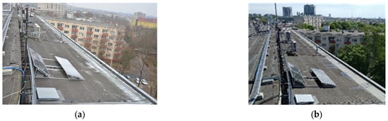
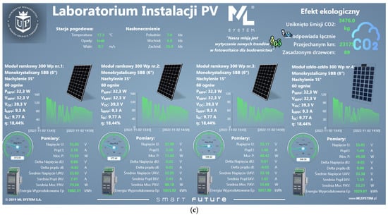
Figure 1.
Examined microinstallation: (a) PV panels in winter; (b) PV panels in summer; (c) interface consisting of the graphical presentation of the current values of key indicators of a functioning photo-voltaic system.
The impacts of selected environmental parameters and particulate matter deposit have been quantitatively and qualitatively analyzed; dust and anthropogenic particle pollution and their impact on the solar flux that is available for power generation by photovoltaic panels were taken into account. The amount of energy that was produced was theoretically estimated and experimentally tested, and the losses in the power that was generated by photovoltaic panels as related to air pollution were estimated on the basis of the experimental data [17,18].
The amounts of pollutants in the air are constantly increasing. An approach to air quality is to pay attention to the processes that lead to the formation of pollutants. Producing less energy from sources that have a destructive effect on the state of the atmosphere is the solution to this problem. Pollution adversely affects the amount of energy that is produced in photovoltaic installations [19].
PV systems have entered the era of artificial intelligence and machine learning. The integration of ICT, 5G, and intelligent systems with photovoltaic systems ensures higher economic efficiency and better operation of the investment. The implementation of the Internet of Things solutions concerns the PV production, installation design (installation selection, meteorological data modeling), and operation stages.
Related Literature and Studies
Environmental factors are very important in this respect. The increase in urbanization, the development of industry, and the use of fossil fuels all cause poor air quality as a consequence, which is one of the most serious problems in the world [20].
When conducting a literature query, the published works can be classified into two main groups: those that perform a prediction, and those that describe the obtained measurements. Predicting the photovoltaic system properties and modeling of PV output by evolutionary algorithms is very popular. The authors in [21] described the parameters for a photovoltaic model that were extracted using three evolutionary algorithms: a genetic algorithm (GA), particle swarm optimization (PSO), and differential evolution (DE). The accuracy and speed of the calculations were compared with the relative errors in the separated parameters based on three techniques under a noise condition. The authors concluded that particle swarm optimization (PSO) showed the highest precision and outstanding anti-noise ability; therefore, there is a proposed computational method to evaluate and extract the parameters of a dye-sensitized solar cell model.
The authors in [22] presented an improved evolutionary computational algorithm to extract a photovoltaic design of parameters using an adaptive genetic algorithm. In order to find the optimal photovoltaic parameters, an approach for matching the current–voltage curve was used. This article presented an improved algorithm of evolutionary computation called the adaptive genetic algorithm (AGA), which is an optimization measure that is based on curve fitting. Two objective functions that were presented in the paper (least mean square error [LSE] and Pearson residual error optimization [PRO]) were considered to fit the curve of the analyzed characteristics.
The work in [23] presented the use of numerical techniques based on genetic algorithms (GA) to identify the electrical parameters of photovoltaic cells and modules. These parameters were used to find the maximum power point from the current–voltage characteristic. The genetic algorithm approach was used as a numerical technique in order to overcome the problems that are associated with local minima. The race of the algorithm stopped after five and seven generations for the solar cells and solar modules, respectively. The identified parameters were used to make a distinction of the maximum power operating points for a photovoltaic cell and module.
The work in [24] presented a method to extract the model parameters of illuminated solar cells based on genetic algorithms. The mathematical description of the solar cell model was determined using the Lambert function. The paper showed the effects of testing the ability of the method that was proposed by the authors compared to the direct extraction method. This test was related to matching the current–voltage characteristics of a selected photovoltaic cell to randomly generated parameters; the obtained accuracy of the results of the proposed method was satisfactory.
Genetic algorithms and genetic programming, differential evolution, evolution strategies, and evolutionary programming are stochastic techniques, so a different result can be obtained each time an algorithm is run. A literature review that describes the obtained measurements will be limited to analyzing the influence of the existing atmospheric phenomena on energy that is produced by photovoltaics. The published works that analyze the obtained measurements that deal with large reductions in solar energy production due to particulate air pollution are mainly not connected to GAs.
The work in [25] presented a study of the effect of dust settlement on energy production by photovoltaic modules using the modified angular loss coefficient. The mathematical method was applied and modified in order to obtain a better prediction of the angular loss coefficient. In the works by [26,27,28,29] on the impact of smog factors on photovoltaic power, the impact of environmental factors on the efficiency of photovoltaic systems was shown; these concluded that solar irradiance has the greatest impact on the efficiency of photovoltaic systems. In [30], the numerical simulations of a PV module were performed; the simulations were performed by computational fluid dynamics (CFD). The numerical results were compared with the experimental results. The influence of the dust deposition density on the electrical and thermal parameters of a photovoltaic module was investigated. The effect of dust, humidity, and air velocity on the performance of photovoltaic cells was mainly investigated by an experimental study in which the dust that was deposited on PV panels was analyzed. The work in [31] presented the results of research on the influence of dust pollution on the permeability of the glass cover of a PV module. The research covered the influence of dust pollution on the total permeability of flat glass and the spectral transmittance of glass with an anti-reflective coating; also, the physicochemical properties of the dust particles were characterized. A dust particle chemical element analysis was carried out using a TESCAN Field Emission Scanning Electron Microscope and a BRUKER X-ray Fluorescence. EDS and XRF chemical element analysis and XRD qualitative and quantitative analysis were used. The influence of humidity on energy losses were estimated; the results that were obtained from this study can be used to size a PV system to meet a specific load and to maintain its required power output by taking the dust effect into account. Similar analyses of this type can be found in [32,33,34,35].
The work in [36] presented genetic algorithms in real problems as a popular field of research on the optimization problems. In the field of energy, many evolutionary approaches have been used; therefore, it is not possible to identify one as the best for the selected issue. The literature on evolutionary algorithms in general and their industrial applications is extensive, but not all of them apply to applications that have found their practical use. The prepared paper aims to apply genetic algorithms in the practice of energy production. Compared to other methods, it has been noticed that genetic algorithms may be a very efficient technique to estimate the influence of particulate air pollution on the electrical parameters of photovoltaic modules.
A genetic algorithm with crossover and mutation was used to estimate the relationship between air pollution and cloudiness with the power that was generated in a photovoltaic installation. The research showed the influence of anthropogenic factors on the power that was generated by photovoltaic panels; therefore, it can be said that this work may start a discussion in this regard but not end it or confine thematic deliberations in this regard [37,38,39].
2. Materials and Methods
2.1. Concept of Measurements
The analyzed site has a specific location because it is in a valley; its air pollution comes not only from local pollution sources (industrial plants, households, and car exhaust fumes) but also from neighboring regions. The predominant directions of the movement of the pollutants are meridional (from west to east), and the pollutants are generally blown in. Since the analyzed location is in a valley, these pollutants remain for a longer period of time. The particles are defined by their diameters even though they differ in size, shape, and chemical composition. The particles may contain carbon, metal compounds, and organic and inorganic compounds.
The aim of the analyses was to determine as a percentage share how air pollution (particularly PM2.5 and PM10 dust particles) adversely affected the production of electricity from solar radiation energy (which must travel through these pollutants). The work is an attempt to answer the question of how much energy is absorbed and reflected by dust in the air. The cloud cover absorbs a certain amount of energy; however, it can be concluded that the share of these components was significant based on the obtained results that showed constant values of energy losses that were caused by the cover of clouds and dust. The share of the sum of the dust in reducing the amount of energy that fell on the ground surface was relatively constant regardless of the analyzed particle size; only the proportions of the share of individual dust fractions changed.
The results showed the impact of pollutants that were composed of small droplets of liquid, dry solid fragments, and solid cores with liquid coatings on the energy production of solar radiation energy, so the efficiency of the solar cells and the efficiency of the entire examined system were not taken into account, as the amount of power that was measured at the output of the system was analyzed. At the same time, all of the power that was produced was consumed by the receivers, so the PV cells always worked to obtain the maximum power from the sunlight that was present at the moment. If the system was disconnected from the receiver, then no energy would be given back, energy production would be zero, and the information would be provided to us by the system that supported the PV installation.
During the analyses, we did not model or predict the behavior of the PV system. The aim of the analyses was to calculate how much the dust affected the amount of energy produced and, more precisely, how much more energy we would obtain under the same conditions without contaminating the PV panels with dust. The obtained results were only true for one selected location where the measurements were carried out; if another location with more favorable wind conditions was analyzed (thus favoring the removal of pollutants from the site), then the dust pollution would be removed from the pollution cap above the site. This would affect the amount of energy that would not reach the solar installation and would not be used by it.
The evolutionary algorithm was used to calculate the percentage distribution of the solar radiation absorption by dust, cloud cover, and solar installation. These parameters directly influenced the performance of the photovoltaics. Using the evolutionary algorithm, three coefficients were calculated (i.e., the shares of PM2.5 and PM10 dust particles as well as the cloud cover). The obtained results showed the shares of each of these parameters that influenced the amount of energy that reached the Earth’s surface. Neural networks are commonly used to predict this process, while the use of evolutionary algorithms is less frequent; the obtained results clearly showed that there was some regularity in estimating the amount of energy that was usable and absorbed by obstacles in the atmosphere. The applied evolutionary algorithms gave better results in the data analysis, while they were worse for the prediction. The results obtained as a result of analyses with evolutionary algorithms can be used to optimize the processes, analyze the obtained data, and find any relationships between them. For prediction, more-accurate results can be obtained by using neural networks (according to the authors’ experience). During the analyses, the process coefficients were identified.
When conducting the analyses in a search for the best solution to the problem that featured three variables (PM2.5, PM10, and cloud cover), the extreme of the function was searched for in our work (i.e., the smallest differences of the subtotals). Various algorithms can be used to accomplish this difficult task. A probabilistic algorithm was used to carry out the task of obtaining an approximation of the best solution. The used evolutionary algorithm is a random algorithm that mimics the natural processes of genetic inheritance. The ongoing evolutionary process corresponds to searching a space for potential solutions, which is possible thanks to the use of the best-available solutions and a broad search of the space for potential solutions. By searching the space for possible solutions with individuals that are evenly distributed in a 3D space at the initial stage of the analysis, a solution cloud was obtained that focused on global extremes. Each subsequent iteration of the program brought the solution closer; consequently, the operation of the algorithm led to the identification of the extremes. As a result of the mutations and crossovers, we obtained an evaluation function that was calculated from the average number of obtained individuals that were clustered around the global extremes; then, we stopped the algorithm. In the history graph, we could observe this by flattening the algorithm. The algorithm was convergent. Ten starts of the algorithm operation were selected to show that, despite the fact that the beginning of the algorithm operation was randomly different each time because we used a random number generator, the obtained results showed similar values. We had a concentrated solution cloud, so the proposed algorithm was convergent (thus, it was well-designed. Moreover, the algorithms that were proposed for searching for the best solution did not give a solution that was worse than 5% of the optimal value; this means that we obtained a slightly worse solution (but not worse than 5% of the best solution). If the calculations were made for a many-times-greater number of generations, then we would obtain a relatively slightly higher approximation to the optimal value over a much longer period of time. Another potentially applicable method is the gradient method; the result of this depends on the starting point of the calculations. However, there is then a risk of locating the local minimum while we are looking for the global minimum.
When performing numerical analyses, there is a danger of finding the local mini-mum. We searched globally, and we had three variables; on this basis, we looked for the result (i.e., we were looking for the global minimum in 4D space). Evolutionary algorithms make this possible for us.
The panels worked at maximum power; we were not interested in any losses. The results that were obtained at the output of the system were important. We treated the energy-harvesting system as a kind of a “black box”.
The shown periods were averaged to one day, so the results for the PM2.5 and PM10 dust particles and cloud cover were averaged to one day. There was some inaccuracy, but it was averaged; the obtained results were not inferior to the results that were obtained from the shorter period for the higher frequency of the measurements [40].
2.2. Instrumentation and Experimental Facility
The object of the research was a photovoltaic microinstallation with a rated electric power of 1200 W. The data that were processed in this work came from a monitored experimental photovoltaic laboratory stand (which is shown in Figure 1). The microinstallation was located on the roof of the fifth floor building of Krakow Pedagogical University. For the period of the analyses that are presented in this work, two panels were inclined at 35°, two were inclined at 15°, and all faced due south (0° S). The analyzed photovoltaic microinstallation was combined with standard photovoltaic modules that were manufactured by ML System S.A. Zaczernie, PL (ML-S6MF/T1-300-992/1639, Zaczernie, Poland).
The basic components of the solar cell modules was monocrystalline silicon. The power of the three frame modules and the glass–glass module was 300 Wp, each module consisted of 60 cells and 5 busbars, and the cell size was 6 inches. These panels were characterized by an efficiency rating of 18.44%. At maximum power, their current and voltage were 9.3 A and 32.3 V, respectively. Data from two weather stations that were located near the PV modules (one directly on the solar panel, and the second about 700 m from the laboratory) were used for the analyses. The weather stations measured the following data: location, measurement time, total insolation, insolation from E, W, S, rainfall, temperature, wind speed/direction, altitude of sun, PM2.5, and PM10. To measure the electrical parameters of the tested photovoltaic panels, a computing system was used to measure the current, voltage, power, and electricity that were sent to the grid. The measurement system computed the averaged, maximum, and minimum values as well as the 15-min changes of the parameters. A 30-s scan interval was selected because this is the scanning measurement period on which all of the sensors in the experimental PV microinstallation worked. Of the available data, the PM10/PM2.5 air pollutants, cloudiness, and amount of power that was generated by the solar panels were analyzed [41].
During the dust layer tests, the deposited dust on the tested panels systematically increased; this resulted in a decrease in the amount of energy that was produced by the panel. A lack of maintenance, which consisted of not removing the pollution, was a deliberate procedure to show the functioning of the installation in the constantly growing environmental pollution. The role of the deposited dust was presented where the losses that resulted from the panel contamination of the surface were estimated at an annual average of 5.0687% [42].
During the 1-year cycle of datalogging, several episodes of rain occurred that influenced the amount of energy that was produced in the micro-plant, as this resulted in a reduced amount of dust that was deposited on the panel, thus changing the percentage of the production loss difference due to the dust contamination. All of the activities that were related to the maintenance (or a lack thereof) were intended to reflect the actual operating conditions of the device as much as possible.
2.3. Data Processing
The total data-acquisition period corresponded to the period from 1 January through to 31 December 2021. The first stage of the data processing was to create a database of the records from the sensors that measured the environmental parameters along with the parameters that were determined by the photovoltaic curve; this allowed us to create a database of the operating parameters of the solar microinstallation under real environmental conditions. Then, the impact of the air pollution and cloudiness on the power generation by the solar system that was caused by solar energy reaching the surface of the Earth was assessed on scripts that were created in MATLAB/Simulink. The analyses that were performed using the evolutionary algorithms proved to be useful for assessing the air quality in the environment. These methods of identifying pollutants are becoming more and more popular, and a genetic algorithm can describe real environmental conditions [43].
An evolutionary algorithm was used to predict the impact of the concentration of the selected pollutants and cloudiness on the amount of power that was generated by the photovoltaic panels. The evolutionary algorithm defined an approximate optimization algorithm in which the mechanisms of selection, reproduction, and mutation were applied, and the evolutionary algorithm progressively created new and better solutions, and solved optimization problems. First, it was necessary to calculate/estimate the parameters of the evolutionary algorithm (including the number of crossovers, number of mutations, size of the population, and number of generations) for the algorithm to work properly. The evolutionary algorithm began the search process by creating a population of potential solutions (an individual) that contained information. The information that was contained in the subject was decoded and judged according to a given criterion; then, the individuals that were assessed as the worst were eliminated in each evolutionary algorithm step. This selection did not introduce any new individual to the population. Those individuals that remained after the selection underwent mutation and recombination with the use of the crossover operator. The purpose of this process was to find those areas that were closest to the optimal areas in the search space; this resulted in obtaining new solutions that were used to build the population of the next generation. The condition to terminate the algorithm was a certain number of generations that enabled the achievement of a satisfactory solution [44]. The applied genetic algorithm gradually created solutions and thus was used to solve the optimization problems. In the analyzed case, this allowed us to estimate the dependence of the possibility of using solar energy in the form of electricity that was produced by a photovoltaic microinstallation regarding the concentration of air pollutants in the air [45,46,47,48].
2.4. Simulation of Power Generated in Photovoltaic Installation Depending on Percentage of Pollutants and Cloudiness
An evolutionary algorithm was used to calculate the required coefficients (as shown in Figure 2). Being an optimization algorithm, this evolutionary algorithm found the best solution from the database of the problem solutions. A single solution (called an individual) represented the solution to a problem with the evaluation function.
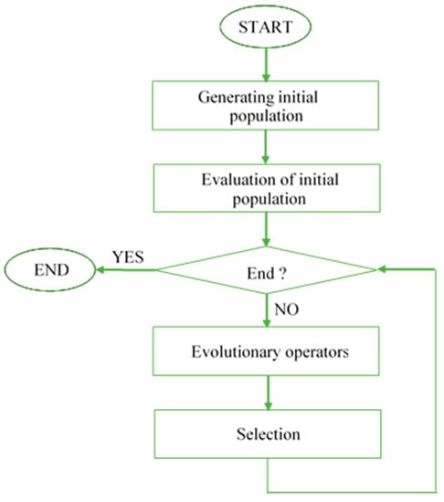
Figure 2.
Evolutionary algorithm flow diagram.
For the three-dimensional case, the individual is marked according to the following formula:
where:
—gene/chromosomes of individual O1;
—value of fitness function of individual O1.
An individual is a vector that consists of four elements: three that are weights, and one that is the fitness function.
Task representation is a way of writing a task formula as a vector of numbers. In the described case, there were four series of measurements that were performed at the same moments of time: power generation from PV panels, amount of PM10, amount of PM2.5, and cloudiness. Each of these series of measurements had different units and different maximum values. First, each waveform value was normalized so that all of the values were within a range of <0.1>. The waveform of the power generation from the PV panels was the base waveform. Each of the three waveforms (PM10 level, PM2.5 level, and cloudiness) was assigned a coefficient. The weight coefficient is a numerical characteristic of the degree of influence of one factor on another. The three coefficients were presented as floating-point numbers from the <0.1> range and were calculated by the evolutionary algorithm. These coefficients made up a single individual as a vector of three elements. The fitness function is given by the following formula:
where:
—value of fitness function for current individual;
N—number of measurement points;
i—current time;
—normalized course of amount of energy produced in i—time, base course;
—normalized PM2.5 mileage in i—time;
—normalized PM10 mileage in i—time;
—normalized course proportional to cloud cover in i—time;
—searched dependency coefficients.
The analyzed population is a fixed set of individuals, the initial population is the set of individuals that are generated and evaluated in the first step of the algorithm, and the new population is the set of individuals that will be in the new generation.
Evolutionary algorithm operators are responsible for generating new individuals, and new individuals are generated based on the current population. Depending on the type (crossover or mutation), the evolutionary algorithm operator selects one or more individuals from the population and processes their coordinates. As a result, a new individual (a new three-dimensional vector) is assigned to which the value of the fitness function is assigned; the newly created individual is then added to the current population.
Selection is responsible for picking up individuals from the current population to the new population that becomes current in the next loop of the program. Selection by the tournament method was used in the analyses. At this point of the algorithm, the basic number of individuals in the population increases with the number of individuals that are generated by the operators of the evolutionary algorithm. The mechanism of this type of choice is based on the selection of three individuals from the current population. The values of their fitness function were compared with those of the new population; the individual with the lowest value of the fitness function was selected. This activity was repeated as many times as the assumed number of individuals in the population.
The Pareto principle defines that 20% of examined objects are related to 80% of resources, so a small part of the causes generate almost all of the effects. In the case of repetitive activities, this principle works well (but it is not always an exact ratio). The Pareto principle is used in engineering to improve the efficiency of analyses; therefore, algorithms are used to calculate the Pareto limit for a finite set of alternatives [49,50,51]. At the beginning of the analyses, the variables that we could measure were identified. These variables were the individuals, generations, mutations, crossovers, and fitness function. Those variables that could generate 80% of the results were determined. The Pareto limit allowed the study to be limited to a set of effective selections and performed analyses within that set rather than considering the full range of each parameter.
The calculations of the relationship between the factors aimed to calculate the percentage dependence of the pollutants and cloudiness on the energy that was produced by the PV panels with the use of an evolutionary algorithm that was initiated by selecting an individual. It was assumed that the O1 individual was randomly selected from the population:
where the results of the evolutionary algorithm calculations are represented by the following:
—weight coefficient of effect of PM2.5 on generated energy;
—weight coefficient of effect of PM10 on generated energy;
—weight coefficient of effect of cloudiness on generated energy;
—fitness function sufficiently that is fast to compute and function that quantitatively measures how fit individuals can be produced from the assumed solution.
3. Results and Discussion
3.1. Visualization of Current, Voltage, and Power Curves of PV Panels
The object of the research was a photovoltaic microinstallation with a rated electric power of 1200 W. Solar cells that were connected in series and/or parallel formed a photovoltaic module, and a photovoltaic system consisted of one or more photovoltaic modules that were connected in series to increase the total voltage. The power that was generated by the PV modules may have been different under the same weather conditions, and the power depended on the point of the current–voltage characteristic. The generated power depended on the obtainable voltage and current; this was the product of the current and voltage. The operating voltage of the tested solar module was 30.3 V, while the operating current was 8.66 A. The power that was obtained during a random day of operation of the installation for one and four tested panels is presented in Figure 3a,b, respectively. Figure 3 shows the diurnal variability of the current, voltage, and power that was generated by the photovoltaic system during a typical spring day at the test location as well as any changes in the meteorological and air-contamination conditions. The set of line and bar graphs that are shown in Figure 3 clearly demonstrate the dependencies between the produced energy and the meteorological data (with data values for each hour of a selected day to analyze the place and day). The line graph in Figure 4a clearly shows the current, voltage, and power that was measured in the PV system that was connected to the electrical grid. There are three graphs in the chart: the brown graph shows the changes in the value of the current during the day; the gray one deals with the changes in the value of the voltage during the day; and the blue graph shows the fluctuations in power during the day. A key significant area was between 9:00 a.m. and 4:00 p.m. From 9:00, the produced energy gradually grew and reached three peaks. At about 11:00, 1:00, and 3:00, there were enormous growths in the power that was generated by the PV modules. During the following periods, the total growth of the power rose to about 170, 160, and 200 W, respectively. From 4:00, the produced energy fluctuated and gradually grew again (although the received increase slowed down). Therefore, we can say that the growth of the power that was generated by the PV modules was generally based on the midday hours. It should first be noticed that the maximum increase in the power that was obtained was much less than the total module power (which reached 300 W). As a consequence, the conversion efficiency had a broad maximum of 68% of the rated power of the PV panel.
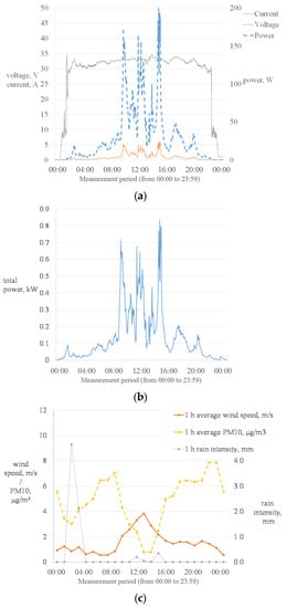
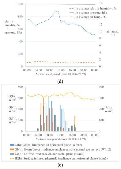
Figure 3.
Fluctuations in the measured parameters that were obtained from the PV system monitoring during one day of measurement period: (a) one panel DC-link voltage, current, and PV panel power; (b) total installation power; (c) air pollution changes with changing wind speed and rain intensity; (d) relative humidity, pressure, and temperature; (e) analyzed day for data from typical meteorological year (TMY) for each hour for analyzed geographic location for selected parameters: G(h), Gb(n), Gd(h), and IR(h).
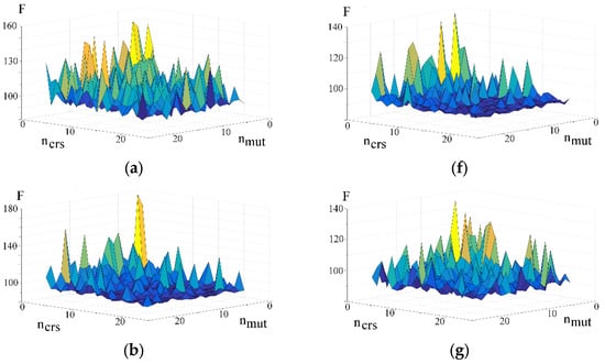
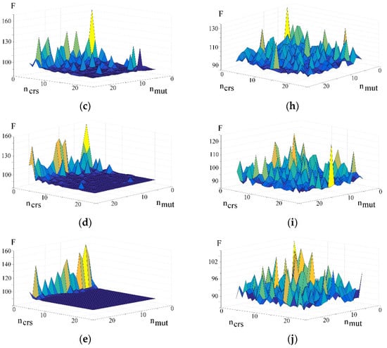
Figure 4.
Effect of changing numbers of individuals and generations in the population of the chosen numbers of mutations (nmut = 0…25) and crossovers (ncrs = 0…25) on fitness function: (a) for 25 individuals in population and for 25 generations; (b) for 25 individuals in population and for 50 generations; (c) for 25 individuals in population and for 75 generations; (d) for 25 individuals in population and for 100 generations; (e) for 25 individuals in population and for 200 generations; (f) for 50 individuals in population and for 50 generations; (g) for 50 individuals in population and for 25 generations; (h) for 75 individuals in population and for 25 generations; (i) for 100 individuals in population and for 25 generations; (j) for 200 individuals in the population and for 25 generations.
The line graph in Figure 3b clearly shows that the four PV panels with the same rated power but with different technologies and positioning generated power that was similar to each other, but it can be noticed that it reached almost 0.79 kW in total against 1.2 kW of nominal power; therefore, they reached an average of almost 70% of the total power. Therefore, the analyzed panel was not optimally positioned in relation to the direction of the solar radiation for the selected hour and day of the year. The next figure (Figure 3c) shows how the air pollution changed with changing wind speeds and rain intensities. The analyzed location was in a valley, so air pollutants flowed down to it; without outside help, they were not able to escape the valley. This is shown in the graph very accurately. Two key significant areas were around 2:00 a.m. and 1:00 p.m. In both cases, the PM10 air pollution decreased significantly. An interesting observation was the beneficial effect of rainfall and wind speed on air quality in a given location; these contributed to the reduction in the amount of dust in the air in such a way that the rain lowered the concentration of the air pollution from 10.51 (the max on the previous day at 7:00 p.m.) to 3.1 µg/m3, and the increasing wind speed caused the pollutant levels to plummet (from 7 to 0.76 µg/m3). If we look at the graph in Figure 3d, one can see that the relative humidity and pressure remained constant throughout the day. What is interesting here is the slight variation in temperatures throughout the day; however, the temperature reached the maximum at around 11:00 a.m. and then dropped steadily. If we look at this and Figure 3b, one will notice that this coincided with the first peak of the maximum power that was obtained by the PV panels. An interesting observation is the graph in Figure 3e; this may partially explain the successive power peaks that were obtained in the PV panels. The graph presents the data for each hour of the day for the analyzed geographic location for the selected parameters:
- G(h)—global irradiance on horizontal plane, W/m2;
- Gb(n)—direct irradiance on plane, W/m2;
- Gd(h)—diffuse irradiance on horizontal plane, W/m2;
- IR(h)—surface thermal irradiance on horizontal plane, W/m2.
An analysis of the graph illustrates the variations in the irradiance during the day. Looking at the global irradiance on the horizontal plane, one can notice a maximum value of 626 W/m2 (which occurred at 8:00 a.m.). Looking at the direct irradiance on the plane that was always normal to the Sun’s rays, one can notice a maximum value of 595 W/m2 (which occurred at 6:00 a.m.). Looking at the diffuse irradiance on the horizontal plane, one can notice a maximum value of 414 W/m2 (which occurred at 1:00 p.m.). Looking at the surface infrared (thermal) irradiance on the horizontal plane, one can note peaks of 347 W/m2 (which occurred at 10:00 a.m., 12:00 noon, and 4:00 p.m.). An evaluation of these data suggested relationships between the power peaks and the surface infrared irradiance. At around 11:00 a.m., 1:00 p.m., and 3:00 p.m., there were increases in the power that was generated by the PV modules. A link can be found with the power peaks shown in Figure 3b, but the relationships were not clear-cut; therefore, we decided to perform the evaluation by numerical techniques using an algorithm that ensured sufficiently good results. Air pollution and cloud cover (which have direct negative impacts on the amount of radiation on the ground surface) were selected as variables.
3.2. Statistical Analysis
The graphs in Figure 4 show the fitness functions for various crossovers and mutations (from 0 to 25). The graphs differ in the number of populations (25, 50, 100, and 200 individuals in the population) and the number of generations (25, 50, 75, 100, and 200 generations) in all combinations. The more individuals in a population and the more generations, the more accurate the results are; however, the computation time will be significantly longer. Too many individuals in a population at these crossover and mutation values will also cause the algorithm itself to converge slowly. The numbers of mutations and crossovers are marked on the horizontal axes in Figure 4a,b. The values of the fitness function according to the numbers of crossovers and mutations are marked on the axes, whereas individuals in the population and generations are outlined in the descriptions. The graphs were smoothed out by increasing the numbers of individuals and generations. A number of 200 generations was assumed for the calculations, which corresponded to the execution of 200 calculation loops; therefore, the values of 100 individuals for 200 generations were selected because the graphs were the smoothest. Computational problems often require taking many criteria into account; two of the most important parameters are the results of the analysis and the calculation time.
We decided to perform a multivariate analysis, the results of which are presented in the graphs that are presented in the series of Figure 4 and Figure 5. These show the influence of four parameters on the calculation results of the evolutionary algorithm. Each point on the value of the plot is the fitness function of the best individual in the evolutionary analysis. As it would be difficult to present the relationships of the four parameters on one graph, the analyses were prepared in stages. Each of the arranged graphs showed two parameters that determine the values of the fitness function. The analyses were carried out for 25, 50, 75, 100, and 200 individuals for each number of generations that were selected for the analysis. The numbers of generations were set at 25, 50, 75, 100, and 200.
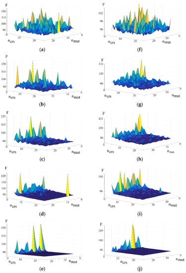
Figure 5.
Effect of the changing numbers of individuals and generations in the population of the chosen numbers of mutations (nmut = 5…25) and crossovers (ncrs = 5…25) on fitness function: (a) for 100 individuals in the population and for 25 generations; (b) for 100 individuals in the population and for 50 generations; (c) for 100 individuals in the population and for 75 generations; (d) for 100 individuals in the population and for 100 generations; (e) for 100 individuals in the population and for 200 generations; (f) for 200 individuals in the population and for 25 generations; (g) for 200 individuals in the population and for 50 generations; (h) for 200 individuals in the population and for 75 generations; (i) for 200 individuals in the population and for 100 generations; (j) for 200 individuals in the population and for 200 generations.
For each variant of the calculations, analyses of the effect of the numbers of mutations and crossovers were carried out—the number of which was initially set from 0 to 25 for each generation. The obtained results led to the determination of the Pareto limit; the selected analyses are presented in the attached graphs. Each plot shows the effect of the numbers of mutations and crossovers (from 0 to 25 per generation). A single drawing is the answer as to how to adjust the number of mutations per generation and the number of crossovers per generation that determines the relationship between these calculation parameters.
The graphs that were obtained as a result of the calculations show the results of the genetic algorithm—each point being a separate evolution with parameters (which can be obtained for 100 individuals, seven mutations, nine crossovers, and 200 generations, for example). The analysis started with the selection of the results that were represented by the graphs that had the most clearly marked wide range of the obtained minimum values. The charts that remained constant and with steady minimums were selected, and another selection criterion was added (which was the trend toward a clear and repeatable minimum). This was conducted to show that, regardless of the moment of starting the genetic algorithm, the results will be very similar. During the initial search, the calculations that obtained the lowest clear values on the graphs were selected. Additionally, the results were selected in which the obtained minimum was as extensive as possible. The result was the selection of several graphs from the analyses that were carried out with a possibly flat and wide minimum area (falling within the assumed 10% tolerance range). The analysis was carried out with 100 individuals and 200 generations (the greater the number of individuals, the greater the excess computation time).
The graph of the calculation results was selected, and the limits of the minimum value range were determined; analyses for the numbers of mutations and crossovers were also performed. The limit of the minimum values was also the assumed Pareto limit. It was observed that for the adopted variant of the choice (for ncrs = 5 and nmut = 20), the final result was also similar to that of ncrs = 5 and nmut = 5, where both variants of the results lay within the area that was limited by the assumed border. The results that were within the minimum area (marked by the yellow line in Figure 6) indicated the same good results because multi-criteria optimization was used and several parameters were examined. An important factor affected the choice of the solution, which also became the computation time. For the selected numbers of individuals and generations, the number of crossovers ncrs = 5 and number of mutations nmut = 5 were selected. The Pareto limit is shown in Figure 6; based on the obtained results, five mutations and five crossovers were selected for further analysis. After analyzing the results that were obtained during the tests, 100 individuals, 200 generations, five crossovers, and five mutations were selected for the calculations.
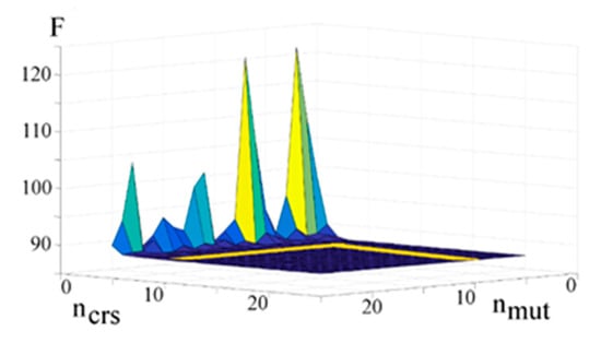
Figure 6.
Fitness function depending on the numbers of mutations and crossovers; yellow line marks the Pareto border.
The parameters of the evolutionary algorithm were calculated on the basis of the experimental data. The assumption of the calculations was to obtain satisfactory results and minimize the calculation time. The characteristics of the value of the fitness function that was calculated for the chosen generation are shown in Figure 7a–c. The line graphs show information about changes in the fitness function over the generations. These graphs show the quality of the evolution and indicate whether the evolution was complete; the results indicate whether the algorithm was convergent. The values in the chart are the fitness function (F) values of the best individual in the analyzed generation. If the curve in the graph decreased slightly, this means that the evolution was considerable and there were no sharp changes in the value; so, gradually, better and better individuals are counted. At the beginning of the evolution, no unique individual was generated that dominated the entire population. The graph that was similar to the e−x function also showed the diversity of the individuals in the population. If this were not true, characteristic sudden dips in the characteristics would be visible.
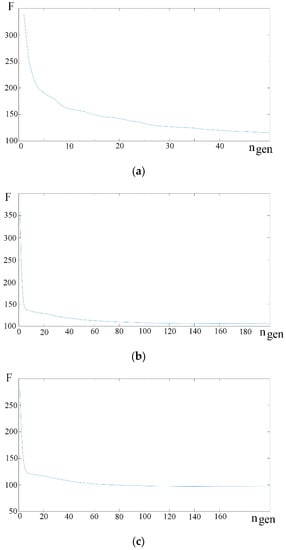
Figure 7.
Plot of fitness function for various calculation variants; analyses were performed for the following: (a) 50 individuals, 50 generations, five mutations, and five crossovers; (b) 50 individuals, 200 generations, five mutations, and five crossovers; (c) 100 individuals, 200 generations, five mutations, and five crossovers.
The curve tended toward the minimum value as the number of generations increased, while the fitness function values steadily decreased. The line graph was characterized by a decrease in the rate of decline as the number of generations increased; this means that the evolutionary algorithm was close to the required minimum. For the analysis that is presented in Figure 7a (50 individuals, 50 generations, five mutations, and five crossovers), the evolution was not complete because the graph did not remain stable in the final phase (gradually decreasing values of the fitness function indicates that the algorithm made no progress). The algorithm was convergent.
For the analysis that is presented in Figure 7b (50 individuals, 200 generations, five mutations, and five crossovers), the evolution was complete; there was a characteristic leveling in the final phase of the curve, but the ending value of the function was higher than that initially assumed (it was above 100). The algorithm was convergent.
For the analysis shown in Figure 7c (100 individuals, 200 generations, five mutations, and five crossovers), the evolution was complete; there was a characteristic leveling out toward a minimum, and it remained stable in the final phase of the curve (the ending value of the fitness function was less than 100). The algorithm was convergent. This was the criterion for selecting the individuals in the population and generations. The 200 generations guaranteed that the evolution for the given parameters was completed (which is shown in the chart by the characteristic remaining constant). The final value (which made it possible to achieve the value of the fitness function that was assumed before the analyses) indicated the sufficient number of 100 individuals.
The surveys that were aimed at calculating the percentage dependence of pollutants and cloudiness on the energy that was produced by the PV panels included data for the entire year. The graphs shown in Figure 8a–c indicate normalized data that were chosen for the random period of 14 February through to 6 March 2021.
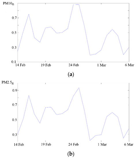
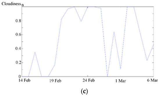
Figure 8.
Normalized changes in the measurement data: (a) PM10; (b) PM2.5; (c) cloudiness.
The normalization of the grades is the adaptation of the values that were measured on the various scales to a conceptually common scale. The result of the calculations of the genetic algorithm for a randomly selected individual O1 was as follows:
Fitness function F was then calculated. Each of the graphs was multiplied by the x1i factors for i = 1…3, and these multiplied plots were added together (as is shown in Figure 9).
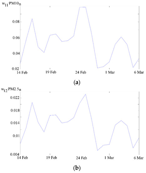
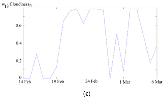
Figure 9.
Normalized changes in the measurement data multiplied by coefficients x1i for i = 1…3: (a) PM10; (b) PM2.5; (c) cloudiness.
The two graphs in Figure 10 show how the fitness function is counted. The red graph is the normalized power graph, while the blue graph is the graph that represents the sum of the graphs: w11 × PM10 + w12 × PM2.5 + w13 × cloudiness. The graphs in Figure 8, Figure 9 and Figure 10 show only a random segment of time, not the entire measurement period (so as not to complicate the drawing with densities of the curves that are too high). The difference between the values on the graph of the normalized power that was generated by the photovoltaic panels and the graphs of the normalized particle concentration in the air around the PV installation and the cloudiness was calculated at each measuring point for each day of the year. The sum of the absolute value of the difference between these graphs was the fitness function value, which was the function by which the individuals were compared. The fitness function is, therefore, the sum of the areas between these curves, which is a numerical value that approximates the value of a definite integral that uses rectangles. There is a connection here: the smaller the difference, the smaller the fitness function value and the better the individual. The graph also clearly shows how the sum of the three graphs (w11 × PM10 + w12 × PM2.5 + w13 × cloudiness) coincides with the graph of the power that was obtained by the tested photovoltaic panels.
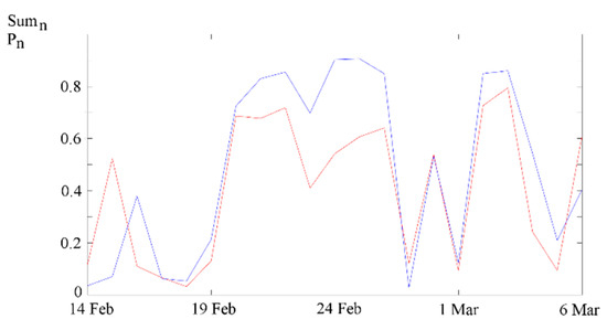
Figure 10.
Graph of the normalized energy that was produced (red line) and the normalized particle concentration and cloudiness multiplied by individual O1 (blue line).
Then, the sum of the absolute values was calculated at each moment during the measurement period, a fitness function parameter was calculated, and the calculation results of the evolutionary algorithm were the following:
The following formula was used to calculate the percentage weight coefficient of the effect relationship:
To calculate the percentage relationship between the amount of pollutants (PM2.5 and PM10) and cloudiness as well as the value of the power that was generated from the solar radiation energy by the photovoltaic panels, an evolutionary algorithm was used with the following parameters:
- number of generations—200;
- population size—100;
- number of crossovers per generation—5;
- number of mutations per generation—5.
The evolutionary algorithm was run ten times for each measurement period; the results of the calculations are presented in Table 1.

Table 1.
Results of the calculations of the evolutionary algorithm for the collected data.
The results of the calculation of the evolutionary algorithm that is presented in Table 1 are represented by the following:
- w%,1 by weight factor of influence of PM2.5 particulate matter on energy that was produced by PV panel;
- w%,2 by weight coefficient of influence of PM10 particulate matter on energy that was produced by PV panel;
- w%,3 by weight factor of cloudiness on energy that was produced by photovoltaic panel.
The results of the calculation showed the influence of PM2.5 (13.38%) and PM10 (2.31%) related to the cloudiness (84.30%) on the power that was generated by the photovoltaic panels. The study calculated the relationship between the air pollution and the cloudiness. Another issue to be analyzed is the determination of the relationships among other factors that influenced the energy production by the photovoltaic panels. Based on the chosen meteorological measurement for the selected location, this will allow us to determine the potential power of the solar panels.
4. Conclusions
The analysis showed how much energy was lost and how to find a solution to best match the power of the PV panels to the customer’s needs and the electricity network. The evolutionary algorithm enabled us to search the space of solutions that avoided the traps of a local minimum. The search for possible solutions in order to find the best (or potentially the best) solution takes place through the mechanisms of evolution and natural selection.
The impact of environmental pollution and cloudiness on the power that was obtained was analyzed with the use of genetic algorithms. During the computation, the algorithms were convergent. The obtained results indicate that the power that was obtained was affected by air pollutants (PM10 and PM2.5 in total) by 15.70% as related to the cloudiness impact. In order to obtain the required power of the solar panels in the analyzed location, they should be equipped with almost 16% more power than was assumed in the project (if only the cloudiness measurements were available). Despite the benefits of free solar energy, solar energy-harvesting systems have disadvantages that include low conversion efficiency, production uncertainty, inconsistency in energy production, and non-linearity in system output power. Their energy production depends on the meteorological conditions and the cleanliness of the atmosphere—on a cloudless and sunny day, the power that is generated by a PV system can be much higher than during a cloudy period (provided there is no dust pollution in the atmosphere above the solar panels, which can effectively reduce the amount of energy that can be produced by the PV panels). To overcome these problems, various optimization and control techniques for manufacturing and operational systems have been proposed to effectively estimate the required power of photovoltaic panels. Genetic algorithms analyze the effects of prior states. They take into account the specificity of electricity production from solar radiation energy, its unpredictability of production, and the influence of many variables on the amount of energy production [52,53,54]. Using the example of the current location, we calculated a loss of about 16% related to the cloudiness.
Analyzing the issue of the reverse, it can be concluded that photovoltaic installations play an important role in the decarbonization of the energy sector, in mitigating the effects of climate change, and in a local positive effect on reducing air pollution (because no harmful substances are emitted into the atmosphere as a result of the electricity-generation process). There are prospects for using such analyses in the future. Assuming less air pollution that can be obtained by modernizing transport systems, limited traffic in city centers for internal combustion vehicles, and fewer people generating airborne particulate matter, the amount of inhalable particulate matter does not have to increase. There are prospects for the development of energy production from PV panels and a more accurate calculation of the amount of energy that will go to the end user that is based on existing pollution and other meteorological component measurements. During the era of the widespread demand for energy, the loss of existing suppliers of energy resources and care for the natural environment by minimizing the emission of a mixture of many chemical species into the atmosphere seem to be extremely important in the context of not only nature, politics, economy, health, and life extension but also financial settlements. Genetic algorithms will play a significant role in this issue.
Author Contributions
Conceptualization—K.P. and W.H.; Methodology—W.H.; Software—W.H.; Validation—K.P.; Formal analysis—W.H.; Investigation—K.P.; Resources—K.P.; Data curation—W.H. and K.P.; Writing/original draft preparation—K.P.; Writing/review and editing—W.H.; Visualization—W.H.; Supervision—K.P.; Project administration—K.P.; Funding acquisition—W.H. All authors have read and agreed to the published version of the manuscript.
Funding
This research received no external funding.
Data Availability Statement
Acknowledgments
This paper and the research behind it would not have been possible without the exceptional technical support of the ML System S.A.
Conflicts of Interest
The authors declare no conflict of interest.
References
- Breeze, P. Chapter 13—Solar Power. In Power Generation Technologies, 3rd ed.; Breeze, P., Ed.; Newnes: London, UK, 2019; pp. 293–321. [Google Scholar]
- Green, M.A.; Dunlop, E.D.; Hohl-Ebinger, J.; Yoshita, M.; Kopidakis, N.; Bothe, K.; Hinken, D.; Rauer, M.; Hao, X. Solar cell efficiency tables (Version 60). Prog. Photovolt. Res. Appl. 2022, 30, 687–701. [Google Scholar] [CrossRef]
- Yoshikawa, K.; Kawasaki, H.; Yoshida, W.; Irie, T.; Konishi, K.; Nakano, K.; Uto, T.; Adachi, D.; Kanematsu, M.; Uzu, H.; et al. Silicon heterojunction solar cell with interdigitated back contacts for a photoconversion efficiency over 26%. Nat. Energy 2017, 2, 17032. [Google Scholar] [CrossRef]
- Cotfas, D.T.; Cotfas, P.A.; Mahmoudinezhad, S.; Louzazni, M. Critical factors and parameters for hybrid Photovoltaic-Thermoelectric systems; review. Appl. Therm. Eng. 2022, 215, 118977. [Google Scholar] [CrossRef]
- ©Fraunhofer ISE: Photovoltaics Report. Updated: 24 February 2022. Available online: https://www.ise.fraunhofer.de (accessed on 1 September 2022).
- m-series-440-435-430-425-420-h-ac-datasheet-539973-revd.pdf. Available online: https://us.sunpower.com/solar-resources/m-series-residential-m440-m435-m430-m425-m420 (accessed on 1 September 2022).
- LG405Q1C-A6. Available online: https://www.lg.com/us/business/neon-r/lg-lg405q1c-a6 (accessed on 1 September 2022).
- REC Alpha Pure Series Product Specification. Available online: https://usa.recgroup.com/sites/default/files/documents/ds_rec_alpha_pure_series_en.pdf?t=1641935533 (accessed on 1 September 2022).
- Geisz, J.F.; France, R.M.; Schulte, K.L.; Steiner, M.A.; Norman, A.G.; Guthrey, H.L.; Young, M.R.; Song, R.; Moriarty, T. Six-junction III–V solar cells with 47.1% conversion efficiency under 143 Suns concentration. Nat. Energy 2020, 5, 326–335. [Google Scholar] [CrossRef]
- Dimroth, F.; Tibbits, T.N.D.; Niemeyer, M.; Predan, F.; Beutel, P.; Karcher, C.; Oliva, E.; Siefer, G.; Lackner, D.; Fuß-Kailuweit, P.; et al. Four-junction wafer-bonded concentrator solar cells. IEEE J. Photovolt. 2016, 6, 343–349. [Google Scholar] [CrossRef]
- Andreani, L.C.; Bozzola, A.; Kowalczewski, P.; Liscidini, M.; Redorici, L. Silicon solar cells: Toward the efficiency limits. Adv. Phys. X 2019, 4, 125–148. [Google Scholar] [CrossRef]
- Webster, R.C. 45—Air Pollution. In Plant Engineer’s Handbook; Mobley, R.K., Ed.; Butterworth-Heinemann: Oxford, UK, 2001; pp. 813–822. [Google Scholar]
- Barichello, J.; Vesce, L.; Mariani, P.; Leonardi, E.; Braglia, R.; Di Carlo, A.; Canini, A.; Reale, A. Stable Semi-Transparent Dye-Sensitized Solar Modules and Panels for Greenhouse Application. Energies 2021, 14, 6393. [Google Scholar] [CrossRef]
- Deolalkar, S.P. Chapter 8—Solar Power. In Designing Green Cement Plants; Deolalkar, S.P., Ed.; Butterworth-Heinemann: Oxford, UK, 2016; pp. 251–258. [Google Scholar]
- Mareddy, A.R. Environmental Impact Assessment: Theory and Practice; Butterworth-Heinemann: Oxford, UK, 2017. [Google Scholar]
- Kuşkaya, S. Residential solar energy consumption and greenhouse gas nexus: Evidence from Morlet wavelet transforms. Renew. Energy 2022, 192, 793–804. [Google Scholar] [CrossRef]
- Pytel, K.; Melnyk, M.; Hudy, W.; Kurdziel, F.; Kalwar, A.; Gumula, S. Predicting the Use of Solar Photovoltaic Panels for Generating Electricity in the Area with Air Pollution. In Proceedings of the 2020 IEEE XVIth International Conference on the Perspective Technologies and Methods in MEMS Design (MEMSTECH), Lviv, Ukraine, 22–26 April 2020; pp. 107–110. [Google Scholar]
- Hudy, W.; Piaskowska-Silarska, M.; Noga, H.; Kulinowski, W.; Pytel, K. Analysis of the possibility of reducing the amount of air pollution using photovoltaic systems. In Proceedings of the 2018 IEEE 19th International Carpathian Control Conference (ICCC), Szilvasvarad, Hungary, 28–31 May 2018; pp. 565–569. [Google Scholar]
- Bergin, M.H.; Ghoroi, C.; Dixit, D.; Schauer, J.J.; Shindell, D.T. Large Reductions in Solar Energy Production Due to Dust and Particulate Air Pollution. Environ. Sci. Technol. Lett. 2017, 4, 339–344. [Google Scholar] [CrossRef]
- Matci, D.K.; Kaplan, G.; Avdan, U. Changes in air quality over different land covers associated with COVID-19 in Turkey aided by GEE. Environ. Monit. Assess. 2022, 194, 762. [Google Scholar] [CrossRef]
- Peng, W.; Zeng, Y.; Gong, H.; Leng, Y.Q.; Yan, Y.H.; Hu, W. Evolutionary algorithm and parameters extraction for dye-sensitised solar cells one-diode equivalent circuit model. Micro Nano Lett. 2013, 8, 86–89. [Google Scholar] [CrossRef]
- Kumari, P.A.; Geethanjali, P. Adaptive Genetic Algorithm Based Multi-Objective Optimization for Photovoltaic Cell Design Parameter Extraction. Energy Procedia 2017, 117, 432–441. [Google Scholar] [CrossRef]
- Zagrouba, M.; Sellami, A.; Bouaicha, M.; Ksouri, M. Identification of PV solar cells and modules parameters using the genetic algorithms: Application to maximum power extraction. Sol. Energy 2010, 84, 860–866. [Google Scholar] [CrossRef]
- Moldovan, N.; Picos, R.; Garcia-Moreno, E.N. Parameter Extraction of a Solar Cell Compact Model using Genetic Algorithms. In Proceedings of the 2009 Spanish Conference on Electron Devices, Santiago de Compostela, Spain, 11–13 February 2009; pp. 379–382. [Google Scholar]
- Zarei, T.; Abdolzadeh, M.; Soltani, M.; Aghanajafi, C. Computational investigation of dust settlement effect on power generation of three solar tracking photovoltaic modules using a modified angular losses coefficient. Sol. Energy 2021, 222, 269–289. [Google Scholar] [CrossRef]
- Gao, T. Photovoltaic Power Prediction Considering the Influence of Smog on Solar Radiation. E3S Web Conf. 2021, 299, 02007. [Google Scholar] [CrossRef]
- Mustafa, R.J.; Gomaa, M.R.; Al-Dhaifallah, M.; Rezk, H. Environmental Impacts on the Performance of Solar Photovoltaic Systems. Sustainability 2020, 12, 608. [Google Scholar] [CrossRef]
- Lin, S.; Chen, N.; Zhou, Q.; Lin, T.; Li, H. A Scheme for Quickly Simulating Extraterrestrial Solar Radiation over Complex Terrain on a Large Spatial-Temporal Span—A Case Study over the Entirety of China. Remote Sens. 2022, 14, 1753. [Google Scholar] [CrossRef]
- Liu, W.; Zhang, J.; Wei, H.; Zhang, K.; Fang, S.; Xie, L.; Ge, J. Short-term PV power prediction considering the influence of aerosol. IOP Conf. Ser. Earth Environ. Sci. 2020, 585, 012017. [Google Scholar] [CrossRef]
- Tao, J.; Zhang, M.; Chen, L.; Wang, Z.; Su, L.; Ge, C.; Han, X.; Zou, M. A method to estimate concentrations of surface-level particulate matter using satellite-based aerosol optical thickness. Sci. China Earth Sci. 2013, 56, 1422–1433. [Google Scholar] [CrossRef]
- Salari, A.; Hakkaki-Fard, A. A numerical study of dust deposition effects on photovoltaic modules and photovoltaic-thermal systems. Renew. Energy 2019, 135, 437–449. [Google Scholar] [CrossRef]
- Said, S.A.M.; Walwil, H.M. Fundamental studies on dust fouling effects on PV module performance. Sol. Energy 2014, 107, 328–337. [Google Scholar] [CrossRef]
- Alnasser, T.M.A.; Mahdy, A.M.J.; Abass, K.I.; Chaichan, M.T.; Kazem, H.A. Impact of dust ingredient on photovoltaic performance: An experimental study. Sol. Energy 2020, 195, 651–659. [Google Scholar] [CrossRef]
- Saidan, M.; Albaali, A.G.; Alasis, E.; Kaldellis, J.K. Experimental study on the effect of dust deposition on solar photovoltaic panels in desert environment. Renew. Energy 2016, 92, 499–505. [Google Scholar] [CrossRef]
- Pulipaka, S.; Kumar, R. Analysis of soil distortion factor for photovoltaic modules using particle size composition. Sol. Energy 2018, 161, 90–99. [Google Scholar] [CrossRef]
- Fountoukis, S.; Figgis, B.; Ackermann, L.; Ayoub, M.A. Effects of atmospheric dust deposition on solar PV energy production in a desert environment. Sol. Energy 2018, 164, 94–100. [Google Scholar] [CrossRef]
- Liagkouras, K. A new three-dimensional encoding multiobjective evolutionary algorithm with application to the portfolio optimization problem. Knowl.-Based Syst. 2019, 163, 186–203. [Google Scholar] [CrossRef]
- Fogel, D.B. Evolutionary Computation: Toward a New Philosophy of Machine Intelligence, 2nd ed.; IEEE Press: Piscataway, NJ, USA, 2000. [Google Scholar]
- Hudy, W.; Pytel, K.; Lobur, M.; Piaskowska-Silarska, M.; Gumula, S.; Melnyk, M. Application of evolutionary algorithms to the analysis of the possibilities of solar energy use. In Proceedings of the 2019 IEEE 20th International Carpathian Control Conference (ICCC), Krakow-Wieliczka, Poland, 26–29 May 2019; pp. 1–6. [Google Scholar]
- Kazem, H.A.; Chaichan, M.T.; Al-Waeli, A.H.A.; Sopian, K. A novel model and experimental validation of dust impact on grid-connected photovoltaic system performance in Northern Oman. Sol. Energy 2020, 206, 564–578. [Google Scholar] [CrossRef]
- Pytel, K.; Hudy, W.; Kurdziel, F.; Kalwar, A.; Gumula, S.; Soliman, M.H. Application of Correlation Analysis for Impact Assessment of Air Quality on the Possibility of Using Chosen Source of Renewable Energy. In Proceedings of the 2020 IEEE XVIth International Conference on the Perspective Technologies and Methods in MEMS Design (MEMSTECH), Lviv, Ukraine, 22–26 April 2020; pp. 17–21. [Google Scholar]
- Alonso-Montesinos, J.; Martínez, F.R.; Polo, J.; Martín-Chivelet, N.; Batlles, F.J. Economic Effect of Dust Particles on Photovoltaic Plant Production. Energies 2020, 13, 6376. [Google Scholar] [CrossRef]
- Mitchell, M.; Taylor, C.E. Evolutionary computation: An overview. Annu. Rev. Ecol. Syst. 1999, 30, 593–616. [Google Scholar] [CrossRef]
- Kuk-Hyun, H.; Jong-Hwan, K. On setting the parameters of quantum-inspired evolutionary algorithm for practical application. In Proceedings of the The 2003 Congress on Evolutionary Computation (CEC’03), Canberra, Australia, 8–12 December 2003; pp. 178–194. [Google Scholar]
- Bhardwaj, R.; Pruthi, D. Evolutionary Techniques for Optimizing Air Quality Model. Procedia Comput. Sci. 2020, 167, 1872–1879. [Google Scholar] [CrossRef]
- Srinivasan, D.; Tettamanzi, A. An Evolutionary Algorithm for Evaluation of Emission Compliance Options in View of the Clean Air Act Amendments. IEEE Trans. Power Syst. 1997, 12, 336–341. [Google Scholar] [CrossRef]
- Saha, C.; Agbu, N.; Jinks, R.; Huda, M.N. Review article of the solar PV parameters estimation using evolutionary algorithms. MOJ Sol. Photoen Syst. 2018, 2, 66–78. [Google Scholar]
- Slowik, A.; Kwasnicka, H. Evolutionary algorithms and their applications to engineering problems. Neural Comput. Appl. 2020, 32, 12363–12379. [Google Scholar] [CrossRef]
- Alhammadi, H.Y.; Romagnoli, J.A. Chapter B4—Process design and operation. In Incorporating Environmental, Profitability, Heat Integration and Controllability Considerations; Seferlis, P., Georgiadis, M.C., Eds.; Computer Aided Chemical Engineering; Elsevier: Amsterdam, The Netherlands, 2004; Volume 17, pp. 264–305. [Google Scholar]
- Jedlicka, P.; Bird, A.D.; Cuntz, H. Pareto optimality, economy-effectiveness trade-offs and ion channel degeneracy: Improving population modelling for single neurons. Open Biol. 2022, 12, 220073. [Google Scholar] [CrossRef] [PubMed]
- Sarver, T.; Al-Qaraghuli, A.; Kazmerski, L.L. A comprehensive review of the impact of dust on the use of solar energy: History, investigations, results, literature, and mitigation approaches. Renew. Sustain. Energy Rev. 2013, 22, 698–733. [Google Scholar] [CrossRef]
- Polo, J.; Martín-Chivelet, N.; Sanz-Saiz, C.; Alonso-Montesinos, J.; López, G.; Alonso-Abella, M.; Battles, F.J.; Marzo, A.; Hanrieder, N. Modeling soiling losses for rooftop PV systems in suburban areas with nearby forest in Madrid. Renew. Energy 2021, 178, 420–428. [Google Scholar] [CrossRef]
- Sulaiman, S.A.; Singh, A.K.; Mokhtar, M.M.; Bou-Rabee, M.A. Influence of dirt accumulation on performance of PV panels. Energy Procedia 2014, 50, 50–56. [Google Scholar] [CrossRef]
- Pérez, N.S.; Alonso-Montesinos, J.; Batlles, F. Estimation of Soiling Losses from an Experimental Photovoltaic Plant Using Artificial Intelligence Techniques. Appl. Sci. 2021, 11, 1516. [Google Scholar] [CrossRef]


Publisher’s Note: MDPI stays neutral with regard to jurisdictional claims in published maps and institutional affiliations. |
© 2022 by the authors. Licensee MDPI, Basel, Switzerland. This article is an open access article distributed under the terms and conditions of the Creative Commons Attribution (CC BY) license (https://creativecommons.org/licenses/by/4.0/).