
Proton-Exchange Membrane Fuel Cell Balance of Plant and Performance Simulation for Vehicle Applications


Abstract
1. Introduction
2. Methodology
2.1. Experimental Setup
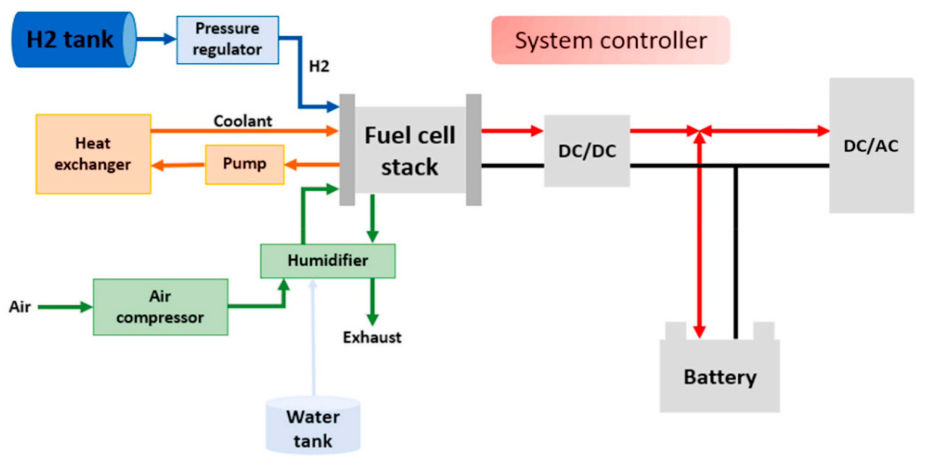
2.2. System Modeling
2.2.1. Fuel Cell Model
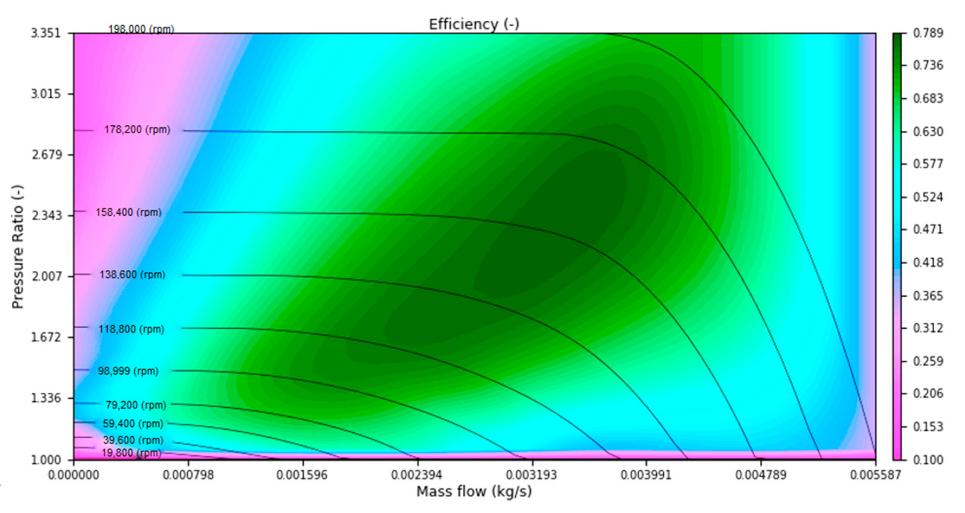
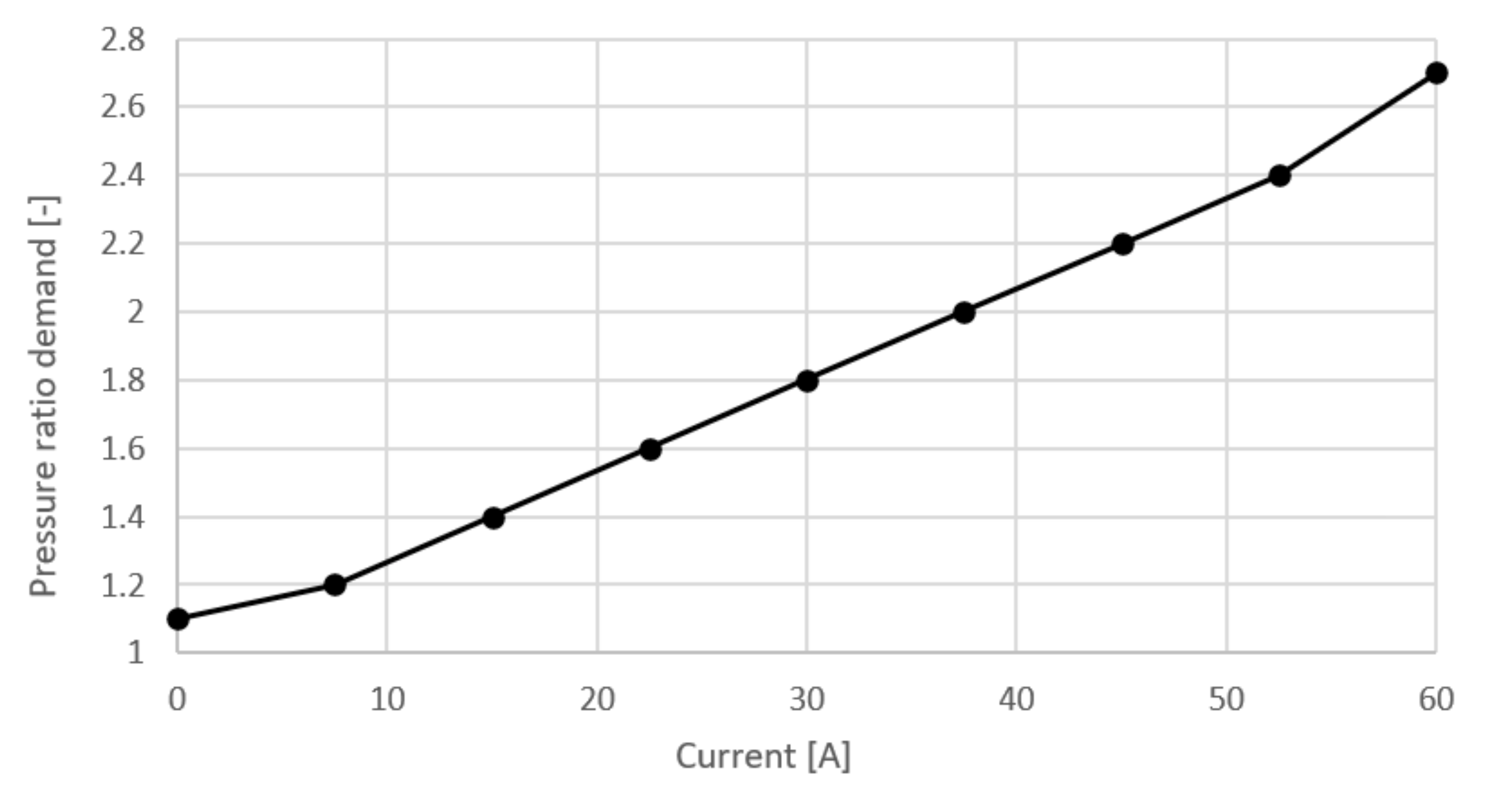
2.2.2. Compressor
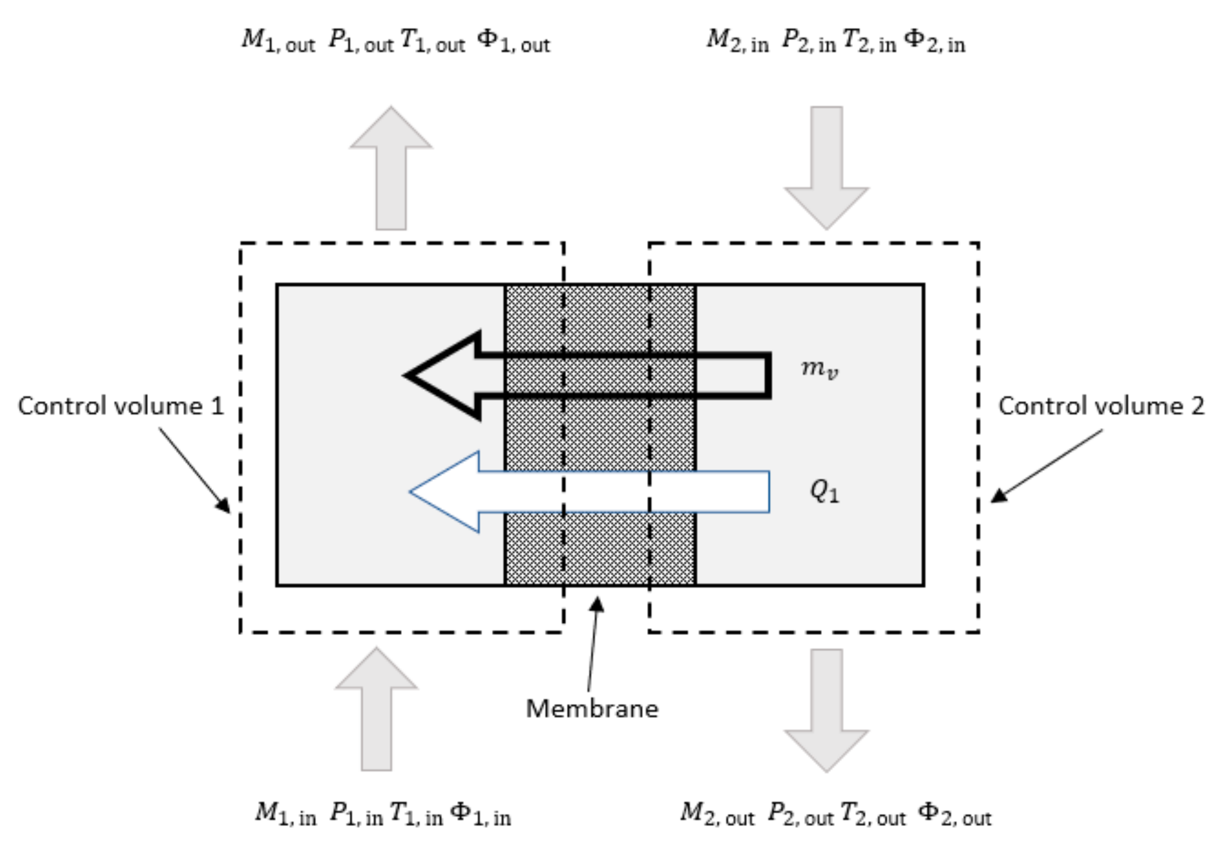
2.2.3. Humidifier
3. Simulation Results
3.1. Base Model Calibration
3.2. Compressor Sizing
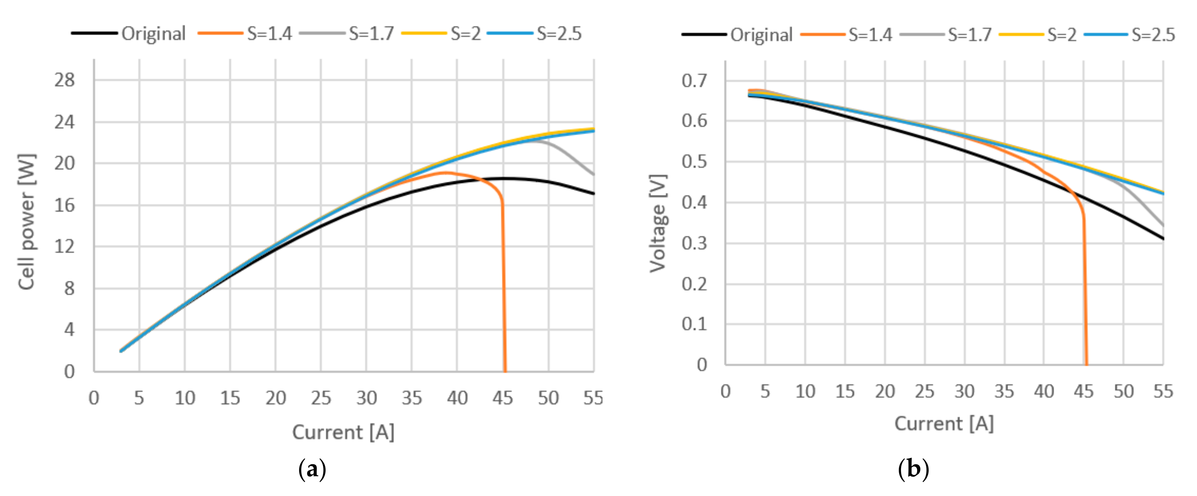
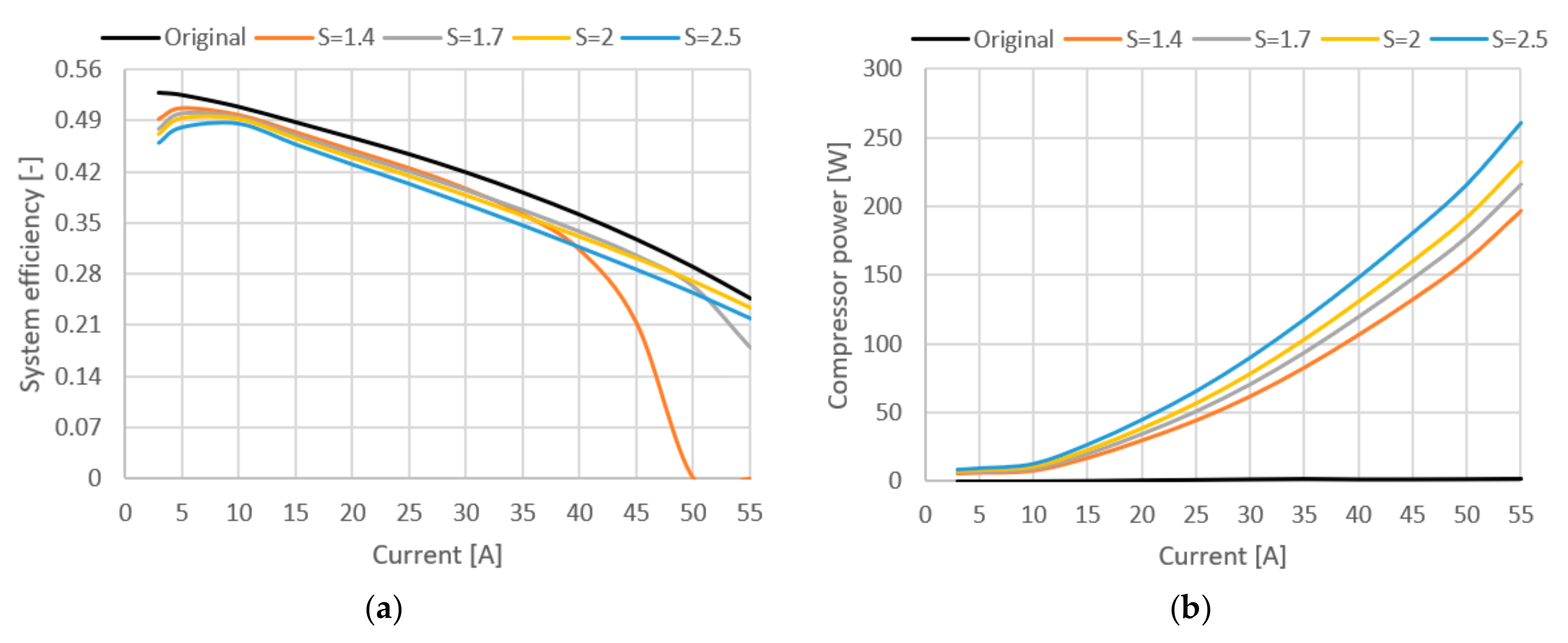
3.3. Simulation Results for Various Stoichometric Ratios
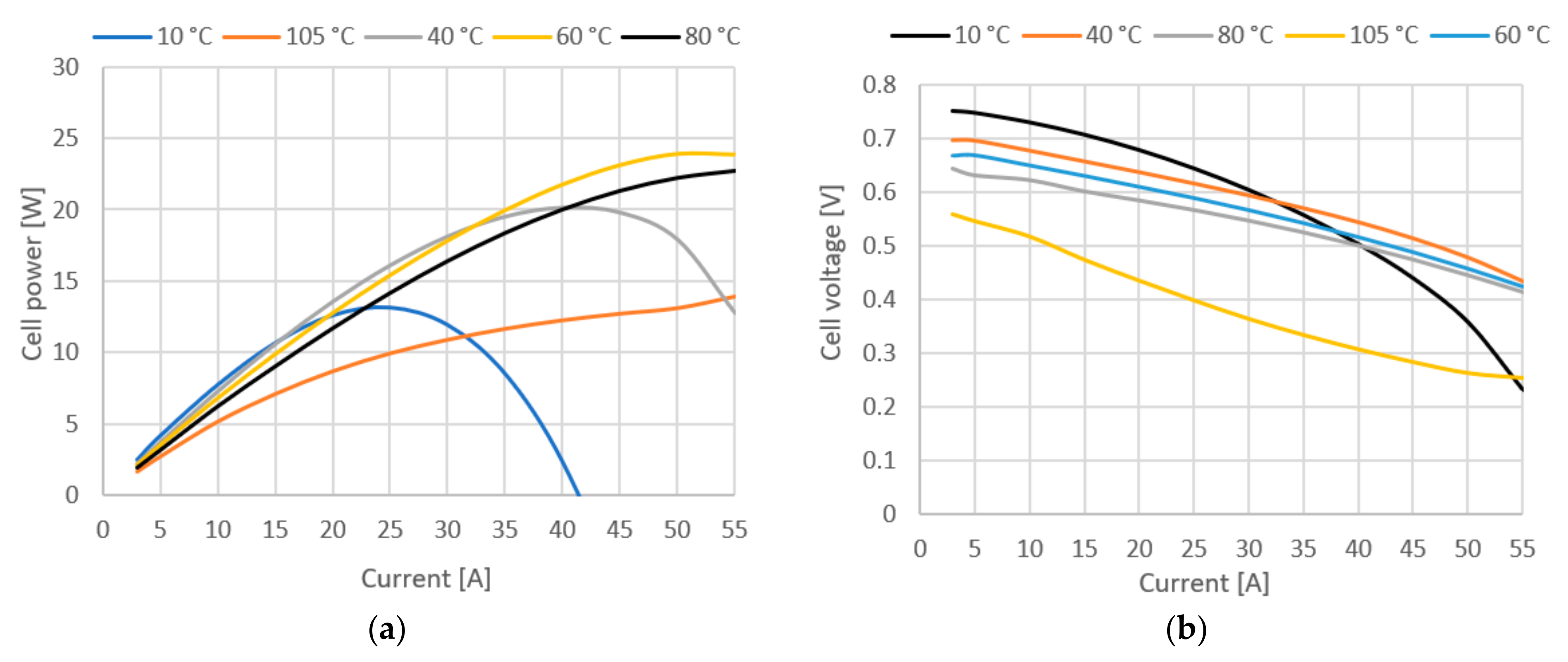
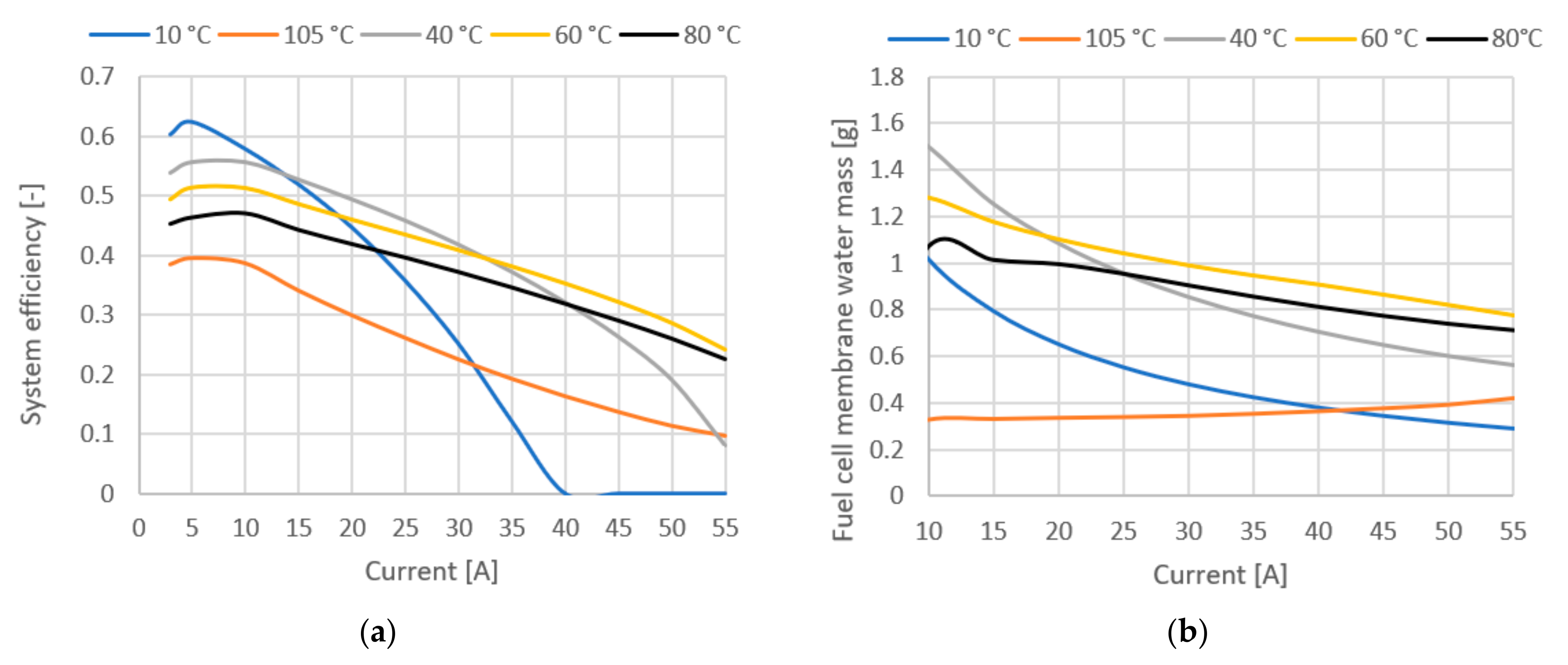
3.4. Simulation Results for Various Stack Temperatures
4. Conclusions
- The cell performance is only slightly changed with the variations in the stoichiometric ratio of the cathode side. The only difference can be seen on high currents (above 45 A).
- Increasing the cell temperature results in increased fuel cell performance at medium to high currents. The optimal working range is determined by the design of experiments and is in the range of 40–60 °C. In future work, a more complex heat and water management system will be applied to the model to see how this auxiliary system affects the efficiency of the overall system.
- In the low current region, due to lower activation losses, low temperature stacks are significantly more efficient (8% difference between 80 °C and 40 °C at 20 A current).
- Compressor addition is justified only in the high current regions where compressor parasitic losses are outweighed by performance gains (22% power gain at maximal load).
Author Contributions
Funding
Conflicts of Interest
References
- Hanif, I.; Raza, S.M.F.; Gago-de-Santos, P.; Abbas, Q. Fossil fuels, foreign direct investment, and economic growth have triggered CO2 emissions in emerging Asian economies: Some empirical evidence. Energy 2019, 171, 493–501. [Google Scholar] [CrossRef]
- Tettey, U.Y.A.; Gustavsson, L. Energy savings and overheating risk of deep energy renovation of a multi-storey residential building in a cold climate under climate change. Energy 2020, 202, 117578. [Google Scholar] [CrossRef]
- Dudley, B. BP statistical review of world energy. BP Stat. Rev. 2018, 6, 00116. [Google Scholar]
- Stolarski, M.J.; Warmiński, K.; Krzyżaniak, M.; Olba–Zięty, E.; Stachowicz, P. Energy consumption and heating costs for a detached house over a 12-year period–Renewable fuels versus fossil fuels. Energy 2020, 204, 117952. [Google Scholar] [CrossRef]
- Jouhara, H.; Olabi, A.G. Industrial waste heat recovery. Energy 2018, 160, 1–2. [Google Scholar] [CrossRef]
- Reitz, R.D. Grand challenges in engine and automotive engineering. Front. Media SA 2015, 1, 1. [Google Scholar] [CrossRef]
- Wilberforce, T.; Baroutaji, A.; Soudan, B.; Al-Alami, A.H.; Olabi, A.G. Outlook of carbon capture technology and challenges. Sci. Total Environ. 2019, 657, 56–72. [Google Scholar] [CrossRef]
- Strielkowski, W.; Lisin, E.; Gryshova, I. Climate policy of the European Union: What to expect from the Paris Agreement. Rom. J. Eur. Aff. 2016, 16, 68. [Google Scholar]
- Böhringer, C. The Kyoto protocol: A review and perspectives. Oxf. Rev. Econ. Policy 2003, 19, 451–466. [Google Scholar] [CrossRef]
- Ma, F.; Wang, Y.; Liu, H.; Li, Y.; Wang, J.; Ding, S. Effects of hydrogen addition on cycle-by-cycle variations in a lean burn natural gas spark-ignition engine. Int. J. Hydrogen Energy 2008, 33, 823–831. [Google Scholar] [CrossRef]
- White, C.; Steeper, R.; Lutz, A. The hydrogen-fueled internal combustion engine: A technical review. Int. J. Hydrogen Energy 2006, 31, 1292–1305. [Google Scholar] [CrossRef]
- Thomas, C. Fuel cell and battery electric vehicles compared. Int. J. Hydrogen Energy 2009, 34, 6005–6020. [Google Scholar] [CrossRef]
- Alaswad, A.; Palumbo, A.; Dassisti, M.; Olabi, A.G. Fuel Cell Technologies, Applications, and State of the Art. A Reference Guide. In Reference Module in Materials Science and Materials Engineering; Elsevier: Amsterdam, The Netherlands, 2016. [Google Scholar] [CrossRef]
- Wilberforce, T.; Olabi, A.G. Performance prediction of proton exchange membrane fuel cells (PEMFC) using adaptive neuro inference system (ANFIS). Sustainability 2020, 12, 4952. [Google Scholar] [CrossRef]
- Wilberforce, T.; Olabi, A.G. Design of experiment (DOE) analysis of 5-cell stack fuel cell using three bipolar plate geometry designs. Sustainability 2020, 12, 4488. [Google Scholar] [CrossRef]
- Sorlei, I.-S.; Bizon, N.; Thounthong, P.; Varlam, M.; Carcadea, E.; Culcer, M.; Iliescu, M.; Raceanu, M. Fuel cell electric vehicles—A brief review of current topologies and energy management strategies. Energies 2021, 14, 252. [Google Scholar] [CrossRef]
- Wang, Y.; Yuan, H.; Martinez, A.; Hong, P.; Xu, H.; Bockmiller, F.R. Polymer electrolyte membrane fuel cell and hydrogen station networks for automobiles: Status, technology, and perspectives. Adv. Appl. Energy 2021, 2, 100011. [Google Scholar] [CrossRef]
- Palencia, J.C.G.; Nguyen, V.T.; Araki, M.; Shiga, S. The role of powertrain electrification in achieving deep decarbonization in road freight transport. Energies 2020, 13, 2459. [Google Scholar] [CrossRef]
- Piraino, F.; Genovese, M.; Fragiacomo, P. Towards a new mobility concept for regional trains and hydrogen infrastructure. Energy Convers. Manag. 2021, 228, 113650. [Google Scholar] [CrossRef]
- de Lorenzo, G.; Andaloro, L.; Sergi, F.; Napoli, G.; Ferraro, M.; Antonucci, V. Numerical simulation model for the preliminary design of hybrid electric city bus power train with polymer electrolyte fuel cell. Int. J. Hydrogen Energy 2014, 39, 12934–12947. [Google Scholar] [CrossRef]
- Shih, N.-C.; Weng, B.-J.; Lee, J.-Y.; Hsiao, Y.-C. Development of a 20 kW generic hybrid fuel cell power system for small ships and underwater vehicles. Int. J. Hydrogen Energy 2014, 39, 13894–13901. [Google Scholar] [CrossRef]
- Pourrahmani, H.; Bernier, C.M.I.; van Herle, J. The application of fuel-cell and battery technologies in unmanned aerial vehicles (UAVs): A dynamic study. Batteries 2022, 8, 73. [Google Scholar] [CrossRef]
- Yue, M.; al Masry, Z.; Jemei, S.; Zerhouni, N. An online prognostics-based health management strategy for fuel cell hybrid electric vehicles. Int. J. Hydrogen Energy 2021, 46, 13206–13218. [Google Scholar] [CrossRef]
- Vichard, L.; Steiner, N.Y.; Zerhouni, N.; Hissel, D. Hybrid fuel cell system degradation modeling methods: A comprehensive review. J. Power Sources 2021, 506, 230071. [Google Scholar] [CrossRef]
- Luciani, S.; Tonoli, A. Control Strategy Assessment for Improving PEM Fuel Cell System Efficiency in Fuel Cell Hybrid Vehicles. Energies 2022, 15, 2004. [Google Scholar] [CrossRef]
- Crespi, E.; Guandalini, G.; Gößling, S.; Campanari, S. Modelling and optimization of a flexible hydrogen-fueled pressurized PEMFC power plant for grid balancing purposes. Int. J. Hydrogen Energy 2021, 46, 13190–13205. [Google Scholar] [CrossRef]
- Staffell, I.; Scamman, D.; Abad, A.V.; Balcombe, P.; Dodds, P.E.; Ekins, P.; Shah, N.; Ward, K.R. The role of hydrogen and fuel cells in the global energy system. Energy Environ. Sci. 2019, 12, 463–491. [Google Scholar] [CrossRef]
- Kravos, A.; Ritzberger, D.; Tavčar, G.; Hametner, C.; Jakubek, S.; Katrašnik, T. Thermodynamically consistent reduced dimensionality electrochemical model for proton exchange membrane fuel cell performance modelling and control. J. Power Sources 2020, 454, 227930. [Google Scholar] [CrossRef]
- Springer, T.E.; Wilson, M.S.; Gottesfeld, S. Modeling and experimental diagnostics in polymer electrolyte fuel cells. J. Electrochem. Soc. 1993, 140, 3513. [Google Scholar] [CrossRef]
- AVL Cruise-M User Manual. Available online: https://www.avl.com/cruise-m (accessed on 29 September 2022).
- Wang, X.; Qu, Z.; Lai, T.; Ren, G.; Wang, W. Enhancing water transport performance of gas diffusion layers through coupling manipulation of pore structure and hydrophobicity. J. Power Sources 2022, 525, 231121. [Google Scholar] [CrossRef]
- Dubose, R. Enthalpy Wheel Humidifiers. In Proceedings of the 2002 Fuel Cell Seminar, Palm Springs Convention Center, Palm Springs, CA, USA, 18–21 November 2002. [Google Scholar]
- Chen, D.; Peng, H. A thermodynamic model of membrane humidifiers for PEM fuel cell humidification control. J. Dyn. Sys. Meas. Control 2005, 127, 424–432. [Google Scholar] [CrossRef]
- Polak, A.; Grzeczka, G.; Piłat, T. Influence of cathode stoichiometry on operation of PEM fuel cells’ stack supplied with pure oxygen. J. Mar. Eng. Technol. 2017, 16, 283–290. [Google Scholar] [CrossRef]


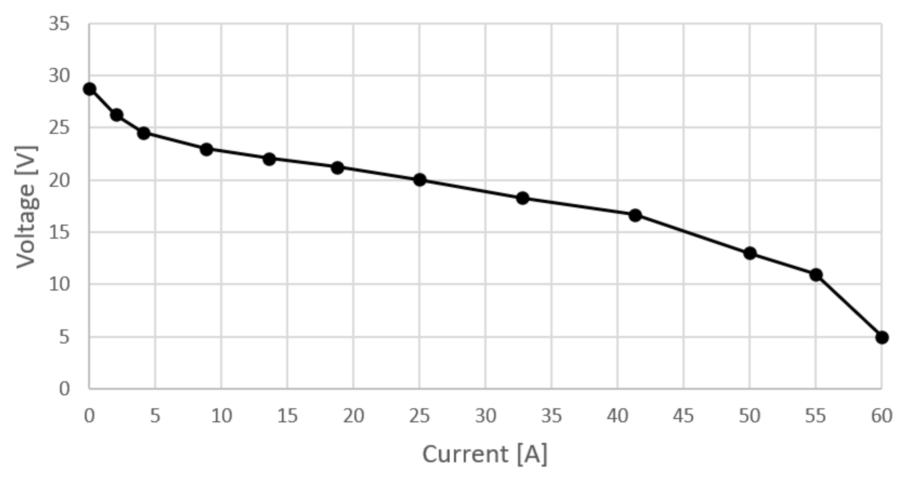
| Power [W] | 100 | 200 | 300 | 400 | 500 | 600 | 687 |
| Current [A] | 4.07 | 8.8 | 13.63 | 18.8 | 24.97 | 32.8 | 41.3 |
| Voltage [V] | 24.55 | 22.98 | 22.09 | 21.24 | 20.04 | 18.3 | 16.7 |
| Ambient air temperature [°C] | 25 | 25 | 25 | 25 | 25 | 25 | 25 |
| Relative humidity [-] | 0.3 | 0.3 | 0.3 | 0.3 | 0.3 | 0.3 | 0.3 |
| Stack temperature [°C] | 38.3 | 40.2 | 41.8 | 42.2 | 43.5 | 44.4 | 45.6 |
| Hydrogen consumption [L/min] | 1.82 | 2.94 | 4.23 | 5.65 | 7.2 | 9.3 | 11.6 |
| Zero Load (3 A) | Operating Point 1 (20 A) | Operating Point 1 (40 A) | Max Load (60 A) | |
|---|---|---|---|---|
| Heat exchanger heat rejection [W] | −1.7528 | 10.32 | 68.506 | 172.03 |
| Temperature after compressor [°C] | 37.451 | 79.915 | 126.1 | 170.66 |
| Inlet mass flow [g/s] | 0.0771919 | 0.514613 | 1.02923 | 1.54384 |
| Pressure ratio [-] | 1.1421103 | 1.5474018 | 2.0948037 | 2.7422055 |
| Humidifier water vapor mass flow [g/s] | 0.00326505 | 0.021767 | 0.043534 | 0.065301 |
Publisher’s Note: MDPI stays neutral with regard to jurisdictional claims in published maps and institutional affiliations. |
© 2022 by the authors. Licensee MDPI, Basel, Switzerland. This article is an open access article distributed under the terms and conditions of the Creative Commons Attribution (CC BY) license (https://creativecommons.org/licenses/by/4.0/).
Share and Cite
Vidović, T.; Tolj, I.; Radica, G.; Bodrožić Ćoko, N. Proton-Exchange Membrane Fuel Cell Balance of Plant and Performance Simulation for Vehicle Applications. Energies 2022, 15, 8110. https://doi.org/10.3390/en15218110
Vidović T, Tolj I, Radica G, Bodrožić Ćoko N. Proton-Exchange Membrane Fuel Cell Balance of Plant and Performance Simulation for Vehicle Applications. Energies. 2022; 15(21):8110. https://doi.org/10.3390/en15218110
Chicago/Turabian StyleVidović, Tino, Ivan Tolj, Gojmir Radica, and Natalia Bodrožić Ćoko. 2022. "Proton-Exchange Membrane Fuel Cell Balance of Plant and Performance Simulation for Vehicle Applications" Energies 15, no. 21: 8110. https://doi.org/10.3390/en15218110
APA StyleVidović, T., Tolj, I., Radica, G., & Bodrožić Ćoko, N. (2022). Proton-Exchange Membrane Fuel Cell Balance of Plant and Performance Simulation for Vehicle Applications. Energies, 15(21), 8110. https://doi.org/10.3390/en15218110