Abstract
Low-grade faults play an important role in controlling oil and gas accumulations, but their fault throw is small and difficult to identify. Traditional low-grade fault recognition methods are time-consuming and inaccurate. Therefore, this study proposes a combination of a simulated low-grade fault sample set and a self-constructed convolutional neural network to recognize low-grade faults. We used Wu’s method to generate 500 pairs of low-grade fault samples to provide the data for deep learning. By combining the attention mechanism with UNet, an SE-UNet with efficient allocation of limited attention resources was constructed, which can select the features that are more critical to the current task objective from ample feature information, thus improving the expression ability of the network. The network model is applied to real data, and the results show that the SE-UNet model has better generalization ability and can better recognize low-grade and more continuous faults. Compared with the original UNet model, the SE-UNet model is more accurate and has more advantages in recognizing low-grade faults.
1. Introduction
At the early stage of fault interpretation, experienced interpreters artificially draw fault lines on the profile according to the discontinuity of the seismic event [1]; however, this method is inefficient and unreliable in accuracy, and manual interpretation is more difficult in areas where geological features are not obvious. With the continuous efforts of geologists, algorithms to automatically recognize faults have been explored. Coherent detection techniques [2,3] recognize faults using the continuity of seismic events. Variance [4] and edge detection techniques [5,6] for fault recognition using discontinuity of seismic events are particularly sensitive to noise and stratigraphic characteristics, are prone to misrecognition, and require extensive manual intervention for modification. Therefore, a series of fault recognition methods such as ant tracking [7,8] and curvature analysis [9] have emerged, which can automatically track faults, but are difficult to apply to different seismic data and cannot be systematically learned and developed based on the experience of interpreters.
The emergence of artificial intelligence has brought fault recognition to a climax. Using deep learning [10,11,12,13,14] for fault recognition overcomes the limitations of traditional recognition methods, efficiently finds the mapping relationship between the input data and target output, and dynamically learns features during the training process. Semantic segmentation has achieved superior application results in the fields of autonomous driving [15,16,17], medical image segmentation [18,19,20,21], and iris recognition [22,23,24]. Semantic segmentation has gradually been applied to seismic fault recognition in recent years. In 2019, Wu et al. [25] used a U-net network for intelligent fault recognition, which achieved end-to-end intelligent recognition of faults. In 2020, Wu et al. [26] used synthetic seismic data to train a full convolutional neural (FCN) network, which, to some extent, avoids the interference of human factors and has a better recognition effect on low-grade faults. In 2021, Liu et al. [27] proposed a 3DU-Net fully convolutional neural network to improve the recognition of small faults in longitudinal profiles and deep noise immunity. Yang et al. [28] and Chang et al. [29] combined a deep residual network with UNet and constructed a network that can accurately recognize the fault location; the recognized faults have adequate vertical continuity. In 2022, Feng et al. [30] proposed a high-resolution intelligent fault identification method, which improved the resolving power of the network model and could detect fault features more accurately.
Convolutional neural networks produce a certain bias in the results when processing local information, so they are combined with attention mechanisms to be able to refer to global information when processing local information. The combination of the attention mechanism and convolutional networks is currently widely used for noise reduction and multiple attenuations. Zhang et al. [31] proposed an attention mechanism-guided deep convolutional self-coding network (AIDCAE), which has more effective noise reduction than traditional methods, is more suitable for desert seismic random noise suppression than mainstream deep learning algorithms, and is competitive in terms of training efficiency. Yang et al. [32] proposed a deep convolutional neural network (GC-ADNet) combining the global context and attention mechanism and suppressing the random noise of seismic data with residual learning, which can effectively suppress random noise and retain more local detailed information. Han et al. [33] fused traditional cyclic generative adversarial networks with an attention mechanism, and the results demonstrated the feasibility of deep learning methods for the processing and interpretation of seismic data. Zhang et al. [34] attenuated multiples using a self-attentive convolutional self-encoder neural network highly correlated with the global space–time of multiples, which proved to be an efficient intelligent processing method for multiple attenuations of real seismic data.
In order to solve the problem of difficult recognition of low-grade faults and low recognition accuracy, this study combines UNet with the attention mechanism SE module [35] to construct SE-UNet with efficient allocation of limited attention resources. In Section 2, we introduce the principle of the SE module and the network structure and characteristics of the self-constructed SE-UNet. This network allocates different learning weights to feature maps through self-learning, which enhances the expression ability of the network and improves the fault identification accuracy. In Section 3, the training workflow is described: sample set construction, preprocessing, network hyperparameter selection, and network model trial calculation. The method proposed by Wu et al. [36] is used to generate 500 pairs of simulated data and corresponding fault labels. Section 4 describes the application of the network model in real data, and further demonstrates the advantages of SE-UNet in identifying low-grade faults by comparing with the results of classical UNet.
2. Methods and Principles
2.1. SE Block
A squeeze-and-excitation (SE) block is a new architectural unit proposed by previous authors to better exploit inter-channel dependencies, and the structure is shown in Figure 1. The channel characteristic response was adaptively recalibrated by explicitly modeling the interdependencies between channels [35]. The SE block consists of two main parts: a squeeze and an excitation. The first step was a squeeze operation to obtain the distribution of the values of the feature maps, which was calculated using Equation (1).
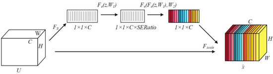
Figure 1.
SE block.
The can be interpreted as a two-dimensional matrix of the Ch channel in the feature maps. and represent the width and height of the feature map, respectively. Equation (1) converts the H × W × C matrix into a 1 × 1 × C matrix. The second step was the excitation operation, which learns the weights of each channel of the feature map through the fully connected layer and the activation function, calculated using Equation (2):
where is the matrix calculated from Equation (1), is the matrix of size 1 × 1 × (C × SERatio), is the matrix of size 1 × 1 × , denotes the activation function, and SERatio is the scaling factor with the purpose of reducing the number of parameters. Finally, the scale operation was performed to multiply the and matrices obtained from Equation (2) to obtain the matrix after updating the weights, which was calculated using Equation (3):
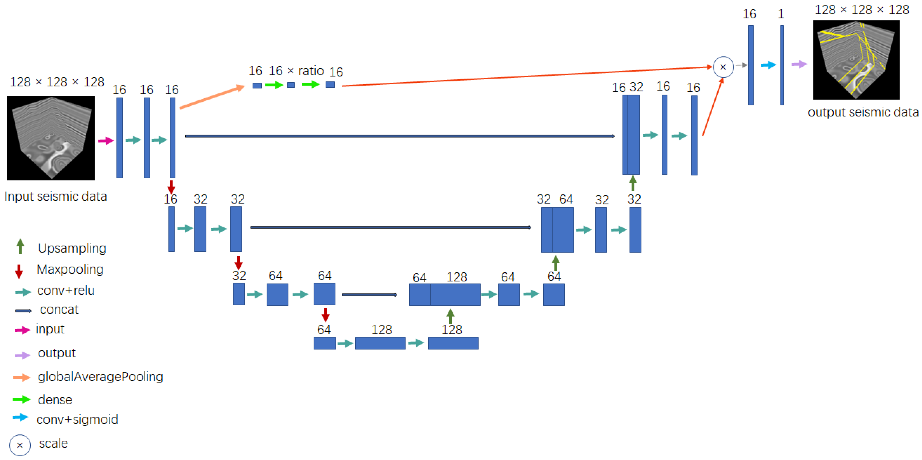
2.2. SE-UNet
UNet is an encoder–decoder structure with a simple and effective structure, where the encoder is responsible for feature extraction and the decoder for up-sampling to recover the original resolution, adding a skip connection between the encoder and decoder to retain the information lost by down-sampling during encoding. Although various features are extracted during encoding, the attention of the network is limited, and limited attention should be paid to the learning of effective features. Therefore, this study combines the SE block with the UNet. The SE block obtains the importance of different channels through self-learning and assigns corresponding weights to each channel according to the learned importance, which makes the network focus on the target characteristics during the learning process, obtains detailed information of the desired target, and suppresses other useless information.
The network structure used in this study is shown in Figure 2, which preserves the encoder and decoder of the UNet structure. The left side of the network is the encoder, which includes three modules, each of which is composed of two convolutional layers and one down-sampling layer. The right side is the decoder, which includes four modules: the first is composed of two convolutional layers, and the remaining three modules are composed of one up-sampling and two convolutional layers. The encoder part performs global average pooling after two convolutions in the first module; that is, the squeeze operation in the SE block. Next, the excitation operation is performed, which consists of two fully connected layers and the activation function, and the SERatio is set to 0.7 to reduce the number of parameters. The output of the fourth module in the decoder part is multiplied by the output of the excitation operation to complete the assignment of the feature map weights. The network only adds two fully connected layers, and the number of parameters remains almost unchanged. This feature has suitable characteristics in terms of the model and computational complexity, and the prediction effect of low-grade faults is significantly improved.
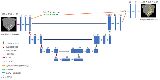
Figure 2.
SE-UNet structure.
3. Model Preparation and Trial Calculations
3.1. Data Preparation
The emergence of artificial intelligence has turned the conventional model-driven methods into data-driven; therefore, we conducted this research under the premise of big data. Low-grade faults are derived from high-grade faults, which are characterized by a fault throw of less than 10 m or an extension length of less than 100 m, and are highly concealed [37]. Owing to the difficulty in obtaining real seismic data, the amount of existing real seismic data is limited and requires manual marking, which is time-consuming and subjective, and is not suitable for use with artificial intelligence methods. This study generated a synthetic 3D seismic record that resembles actual seismic data by using Wu’s [36] method of generating simulated data. The specific steps are as follows.
(1) Construction of a reflection coefficient model. To construct the fold and fault characteristics, we first built the planar initial model with the values of the initial model randomly chosen within [−3, 3].
(2) Adding folding. We simulated the fold structure in a real geological environment by vertically shearing the flat model. Shearing was determined by two shift fields, which are given by the following equations:
The linear shift field of Equation (4) was used to create purely dipping structure, and the values of were chosen randomly. To avoid extremely dipping structures, were chosen randomly within [−0.2, 0.2]. Equation (5) consists of a linear scaling function and 2D Gaussian functions, which were used to construct bending structures with different curvatures, where were given randomly. To avoid generating sharp bending structures, the smaller the is, the smaller the should be.
(3) Fault structures were added based on step (2). A reference point, strike, and dip were given first and used to determine the fault plane; then, a local coordinate system was established with the reference point as the origin and the direction where the fault is located. The point above the fault was then moved, and the equation of the fault throw in the dip direction is shown as follows:
Finally, the data were interpolated. The strike angle was chosen randomly within [30°, 320°], the dip angle was chosen randomly within [35°, 75°], and were given randomly.
(4) The model was convoluted with a wavelet, and noise was added. We convoluted the model obtained in step (3) with the ricker wavelet to ensure the consistency of the synthetic seismic data with the known structural characteristics, and added random noise to the model to ensure the realism of the model data.
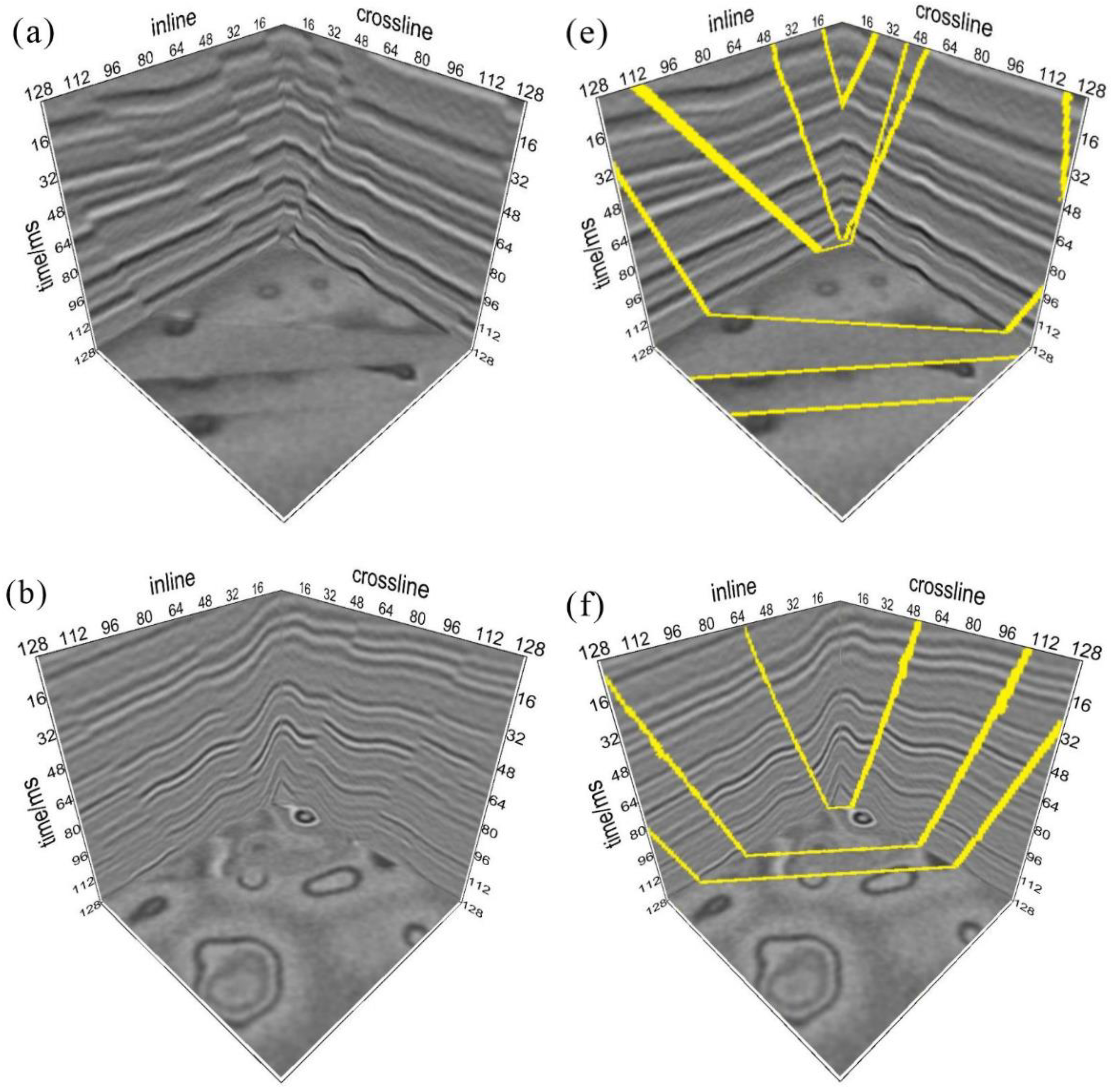
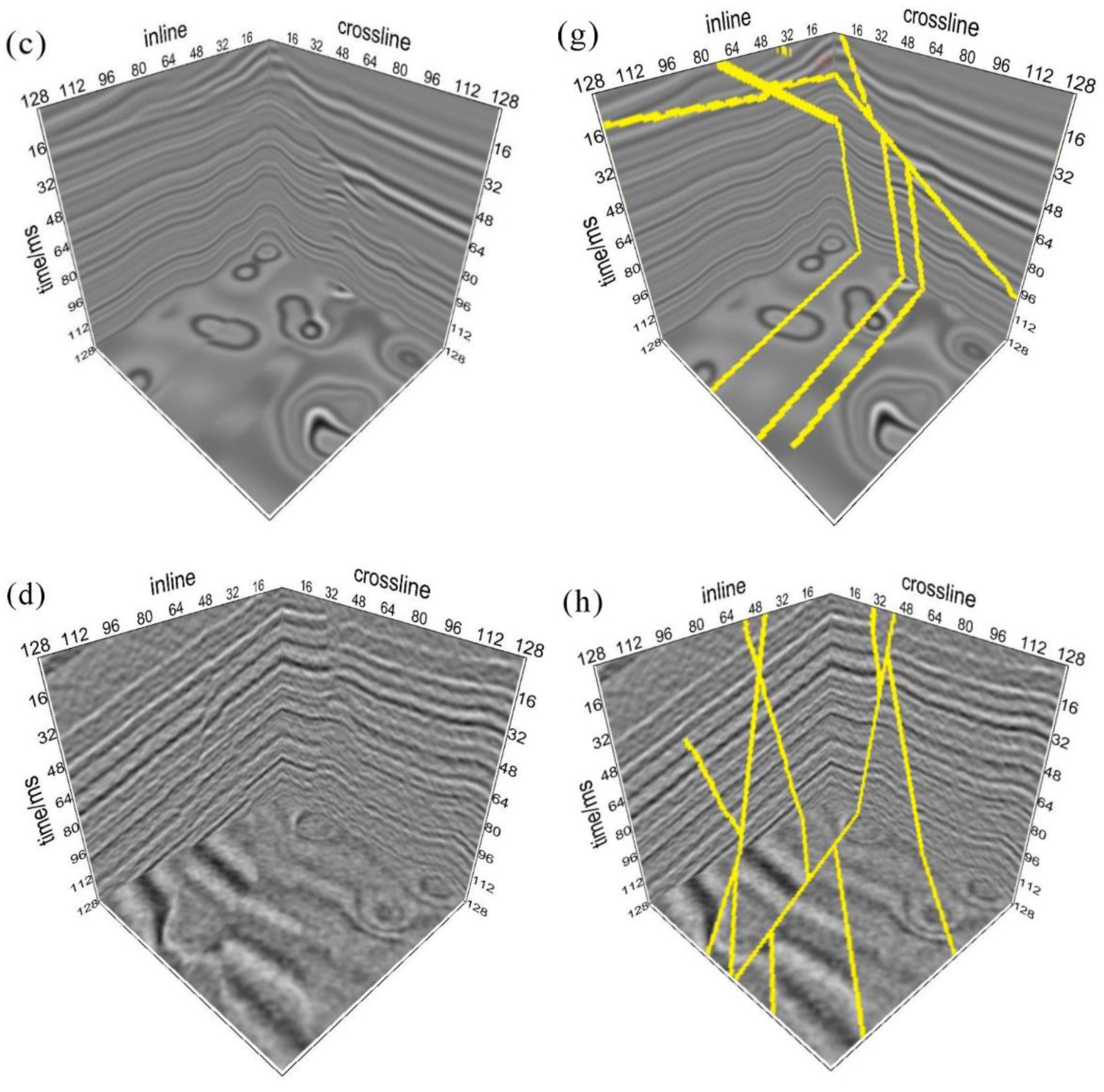
Following the above steps, we generated 500 pairs of synthetic seismic data with dimensions of 128 × 128 × 128. The synthetic seismic data are shown in Figure 3. The sample set contains multiple types of faults: (a) inverse, (b) parallel, (c) conjugate, and (d) normal. (e), (f), (g), and (h) in Figure 3 show the labeled faults of (a), (b), (c), and (d). Low-grade faults are shown in Figure 4 and contain three types of low-grade faults: (a) disconnection, (b) dislocation, and (c) twist types, and (d), (e), and (f) are labels of figures (a), (b), and (c), respectively.

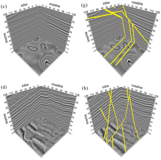
Figure 3.
Three-dimensional synthetic seismic data and fault labeling. (a) Reverse fault; (b) parallel fault; (c) conjugate fault; (d) normal fault; (e–h) are the fault labels of (a–d).
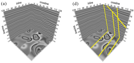
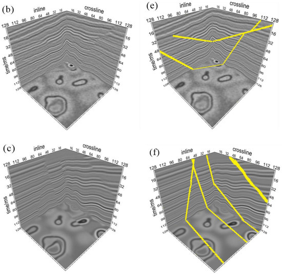
Figure 4.
Three-dimensional low-grade sample set. (a) Disconnection of the seismic event; (b) dislocation of the seismic event; (c) twists of the seismic event; (d–f) are the fault labels of (a–c).
3.2. Data Processing
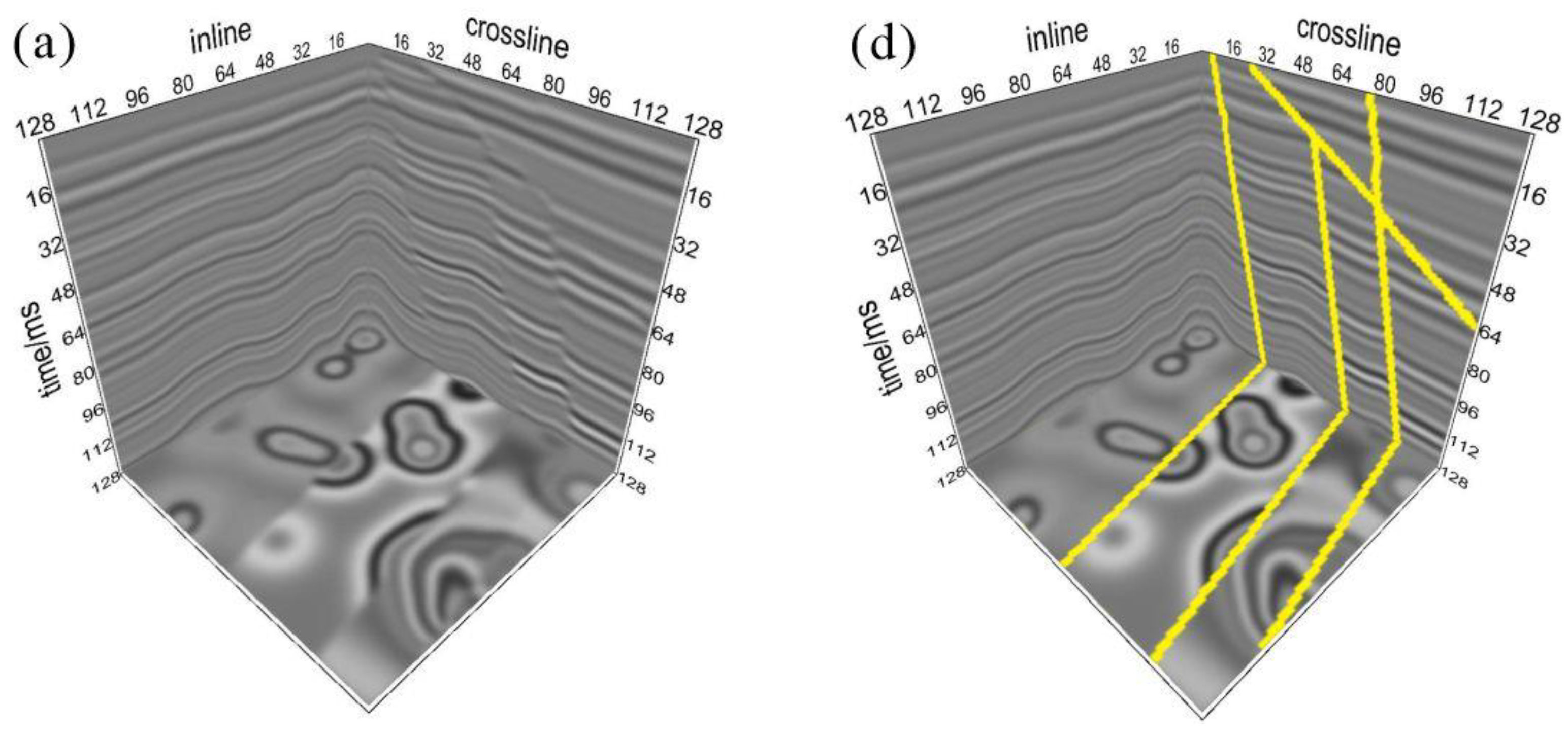
In this study, the data involved in training were processed by random cropping, which crops the data to a random size and then expands them back to the original size. The random cropping method involves reallocating the weight proportion of each feature in the corresponding category, weakening the weight of the background, enhancing the stability of the model, and expanding the dataset simultaneously. The random cropping process allows the network to learn detailed information about the data and observe them over a large sensory field. The data dimension size was 128 × 128 × 128, and the integer value N was randomly taken within [64, 128]. The data were randomly cropped in the first dimension according to the N × N size and subsequently expanded back to 128 × 128 by bilinear interpolation. Figure 5a shows the seismic data, Figure 5b shows the expansion of Figure 5a after cropping the data to 128 × 64 × 64 size, and Figure 5c shows the expansion of Figure 5a after cropping the data to 128 × 96 × 96 size.
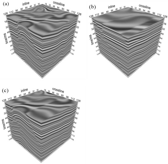
Figure 5.
Data random clipping processing. (a) Simulated seismic data; (b) crop to 64 × 64 and padding; (c) crop to 96 × 96 and padding.
The data were normalized and processed using normalization algorithm S (Equation (7)), which limits the values to a certain range, thus eliminating the undesirable effects caused by odd sample data, speeding up the optimal solution of gradient descent, and improving the accuracy. The S normalization formula is as follows:
where represents the value of a point, and and represent the mean and standard deviation of the data, respectively.
3.3. Network Hyperparameter Analysis and Selection
As the proportion of faults in the data was severely unbalanced, a balanced cross-entropy loss function was chosen in this study to improve the sample imbalance problem. The number of epochs was set to 100. The model was sensitive to changes in the learning rate (lr) and batch size. The lr that affects the convergence degree of the model should be adjusted carefully, so lr was set to 0.001 according to previous experience and fixed. Batch size affects the generalization ability of the model; thus, to improve the generalization capability of model, experiments were conducted using the control variables method to select the optimal batch size, and the network model was evaluated qualitatively using the model evaluation criteria and analyzed quantitatively using the prediction results.
Fault recognition is ultimately a classification task, usually with four types of prediction results (Table 1): true positive, true negative, false positive, and false negative. True positive indicates that the point in the fault label is a breakpoint and predicts it as such; true negative indicates that the point in the fault label is a non-breakpoint and predicts it as such; false positive indicates that the point in the fault label is a non-breakpoint but predicts that the point is a breakpoint; false negative indicates that the point in the fault label is a breakpoint but predicts that the point is a non-breakpoint.

Table 1.
Four prediction scenarios for fault recognition.
Accuracy (Acc) and recall (R) can be used in semantic segmentation to verify the model. The two evaluation criteria are defined as follows:
Acc indicates the ratio of correctly predicted samples to all samples, and is calculated as shown in Equation (8).
R represents the ratio of the number of samples that are true positives predicted to be faults to the number of samples that are actually faults, and is calculated as shown in Equation (9). Therefore, the larger the R value is, the better the model is, and the maximum value of R was 1.
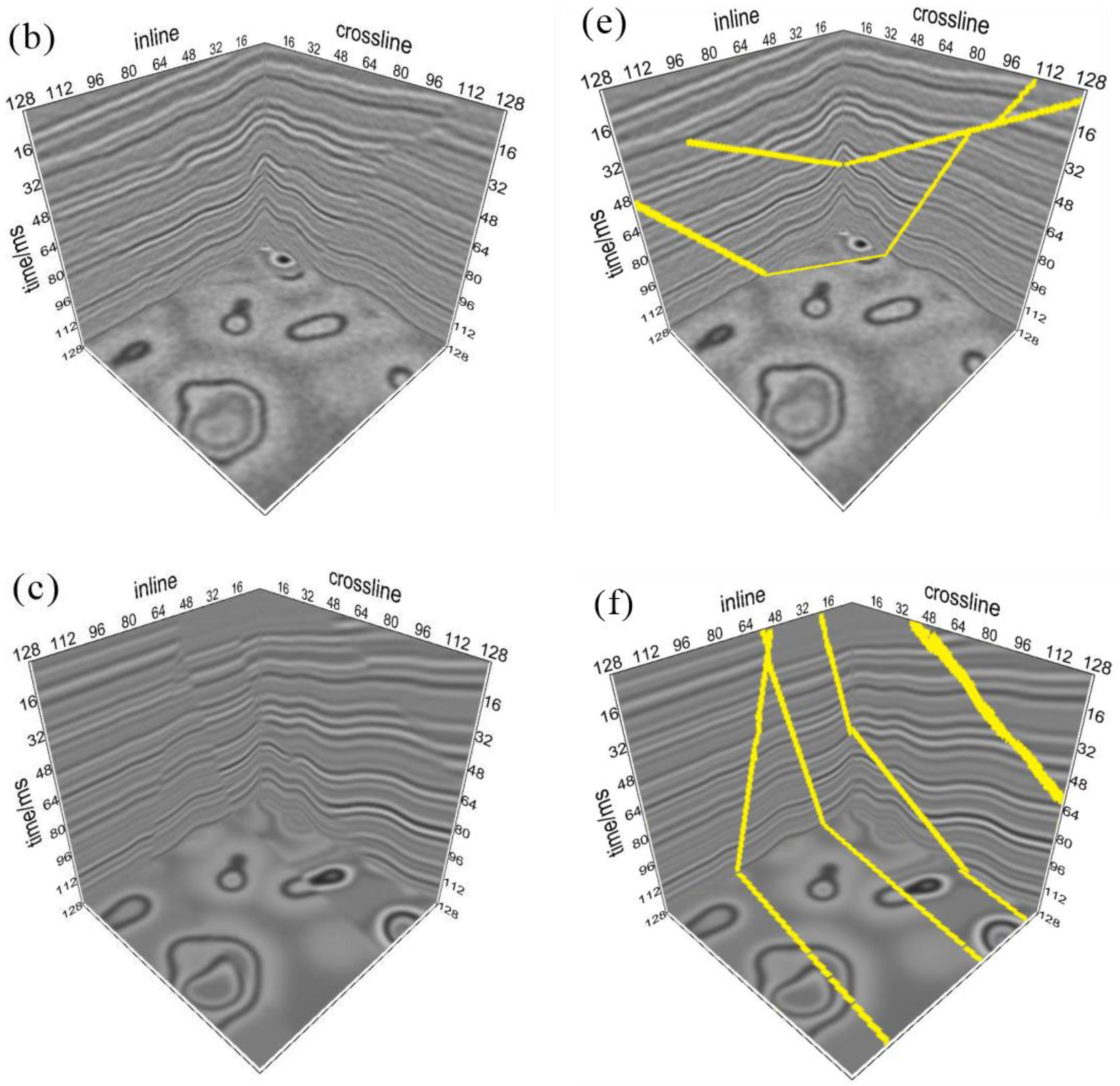
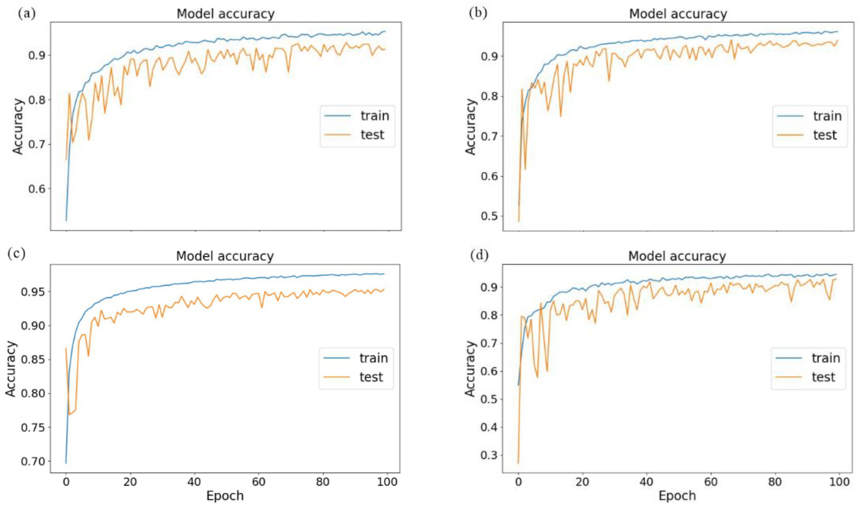
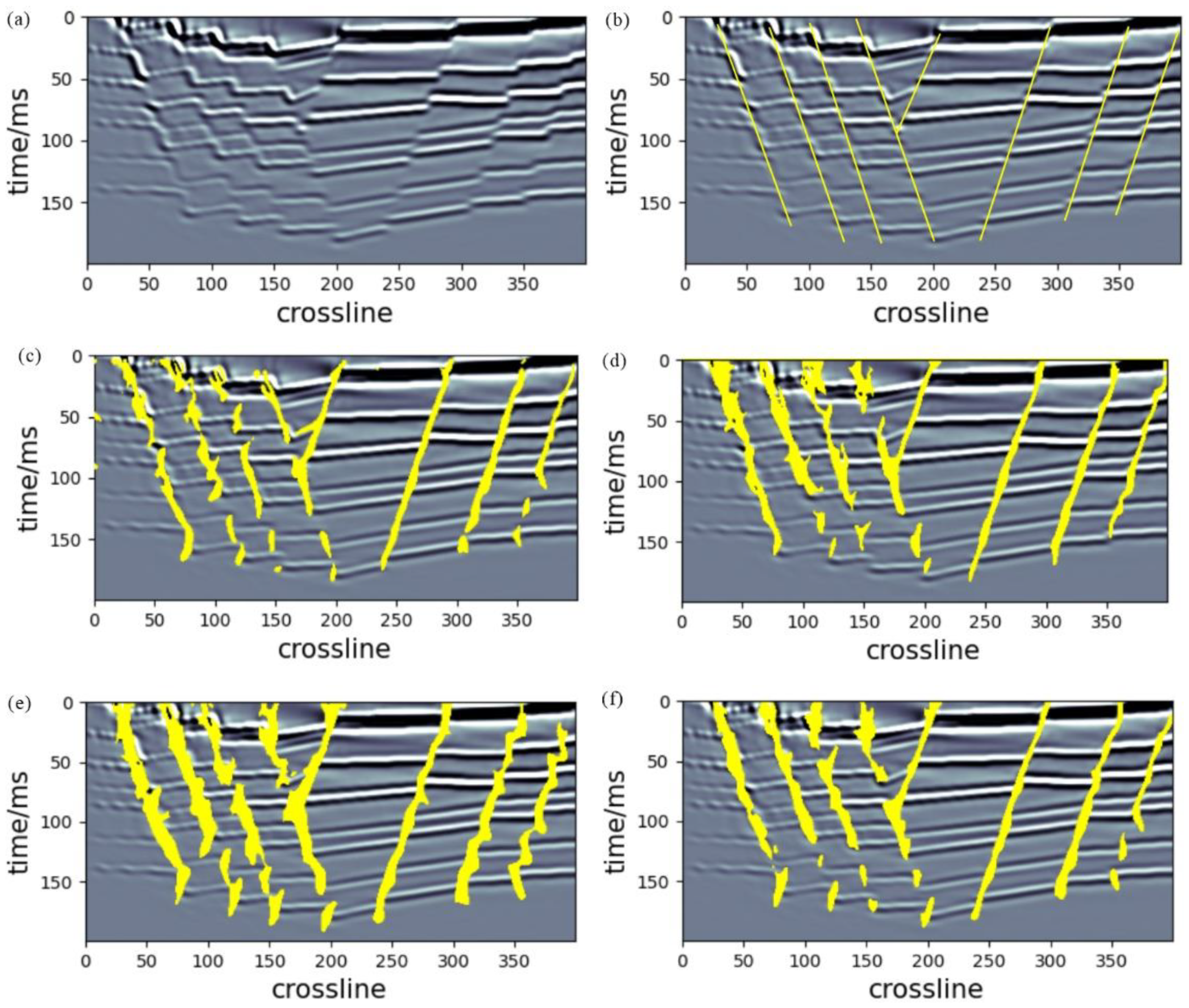
The goodness of fit of the generated models with different batch sizes was evaluated using Acc. The accuracy variation curves of the different batch size generated models are shown in Figure 6. Figure 6a–d represent the model accuracy variation curves when the batch size was 1, 3, 5, and 6, respectively. Analyzed from the Acc perspective, the training accuracy curves of Figure 6a–d changed smoothly, and the model converged stably. The test accuracy of Figure 6c was higher than that of Figure 6a,b,d and the test accuracy curve of Figure 6c was smooth and stable. From the perspective of model generalization ability, the model prediction results are shown in Figure 7, in which (c), (d), (e), and (f) are the prediction effect plots of the model generated with batch sizes of 1, 3, 5, and 6, respectively. Figure 7 clearly shows that the model identified better fault continuity and low-grade level faults when the batch size was 5. Because larger batch sizes require shorter training times and make the computational gradient more stable, the preferred size of batch size was 5, under the premise of ensuring the convergence stability of the network model.
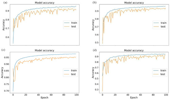
Figure 6.
Model accuracy change curves: (a) batch size = 1; (b) batch size = 3; (c) batch size = 5; (d) batch size = 6.
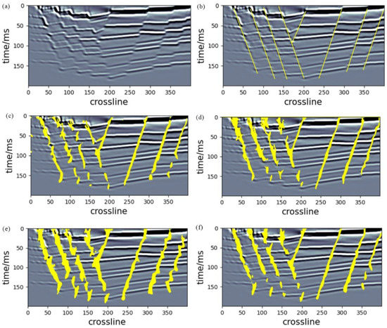
Figure 7.
Model prediction effect diagrams generated using different batch sizes. (a) Seismic profile of Inline10; (b) fault labels corresponding to the Inline10 seismic profile; (c) batch size = 1; (d) batch size = 3; (e) batch size = 5; (f) batch size = 6.
3.4. Model Trial Calculations
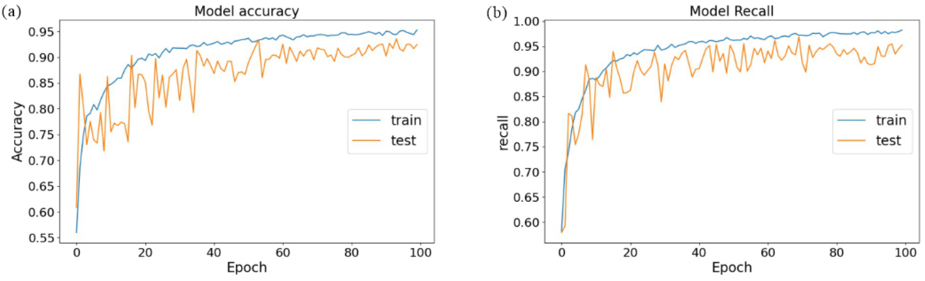
The network parameters (lr = 0.001, batch size = 5, balanced cross-entropy loss function, and epoch = 100) trained SE-UNet and UNet using 500 pairs of simulated data, and tested the model with 100 pairs of data with dimensions of 128 × 128 × 128 (simulated data not involved in training). The models were evaluated using two evaluation criteria, Acc and R. The comparison results are presented in Table 2. The training and testing accuracies and recall of SE-UNet were higher than those of UNet. The curves of the two evaluation metrics with epoch changes for the network and UNet are shown in Figure 8 and Figure 9, respectively. Comparing Figure 8 and Figure 9, we found that the accuracy curve of the model generated by the network changed smoothly, the model converged stably, the recall of the training set of the model was nearly one, and the recall of the test set changed smoothly. The test accuracy fluctuated severely in the accuracy curve of the model generated by the UNet network, indicating that the model generalization ability was weaker than that of the SE-UNet model.
Table 2.
Table of quantitative analysis of the UNet and SE-UNet networks.
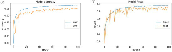
Figure 8.
Acc and R evaluation index curves of SE-UNet. (a) Acc; (b) R.
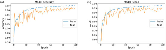
Figure 9.
Acc and R evaluation index curves of UNet. (a) Acc; (b) R.
Random Gaussian noise with various weights was added to the simulated data to verify the noise immunity of the SE-UNet model. The signal-to-noise ratio was calculated using Equation (10). Figure 10a shows the original seismic data and fault labels, and Figure 10b–f shows the seismic data and fault prediction results with signal-to-noise ratios of 20 db, 10 db, 7 db, 6 db, and 5 db, respectively. When the signal-to-noise ratio was higher than 6, the prediction results of the network model were consistent with the fault labels, and there was no missed or incorrect recognition. When the signal-to-noise ratio was lower than 6, the noise slightly interfered with the network model trial calculation, and in the time slice direction, there was missed recognition and no wrong recognition. Overall, the network model in this study exhibited strong noise immunity.
where is the signal-to-noise ratio, is the seismic data without noise, is the seismic data with random noise, is the random noise data, and is the sampling point for the seismic data.
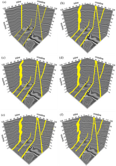
Figure 10.
Results of SE-UNet model predicting different SNR data. (a) Noise-free simulated seismic data and fault labels; (b) simulated seismic data and fault prediction results with SNR of 20 db; (c) simulated seismic data and fault prediction results with SNR of 10 db; (d) simulated seismic data and fault prediction results with SNR of 7 db; (e) simulated seismic data and fault prediction results with SNR of 6 db; (f) simulated seismic data and fault prediction results with SNR of 5 db.
4. Applications
We used the forward and migration methods to generate 200 × 400 × 128 simulated data with low-grade faults. We applied the network model to the simulated data and cleaned the predicted results. The value of fault probability was set higher than 0.7, and the prediction effect is shown in Figure 11. Figure 11a shows the profile of the simulated data inline, where the crossline direction (0–200) had more fault disturbance factors, and the stratigraphy was more blurred. Figure 11b shows the fault labels and Figure 11c,d shows the prediction results of the UNet and SE-UNet models, respectively. The comparison shows that both UNet and SE-UNet could accurately recognize fault locations, but the continuity of the fault results recognized by SE-UNet was better at crossline 0–200.
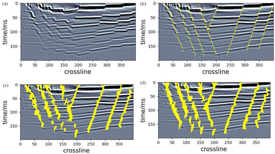
Figure 11.
Prediction renderings of UNet model and SE-UNet model. (a) Seismic profile of Inline10; (b) fault labels corresponding to the Inline10seismic profile; (c) UNet recognition; (d) SE-UNet recognition.
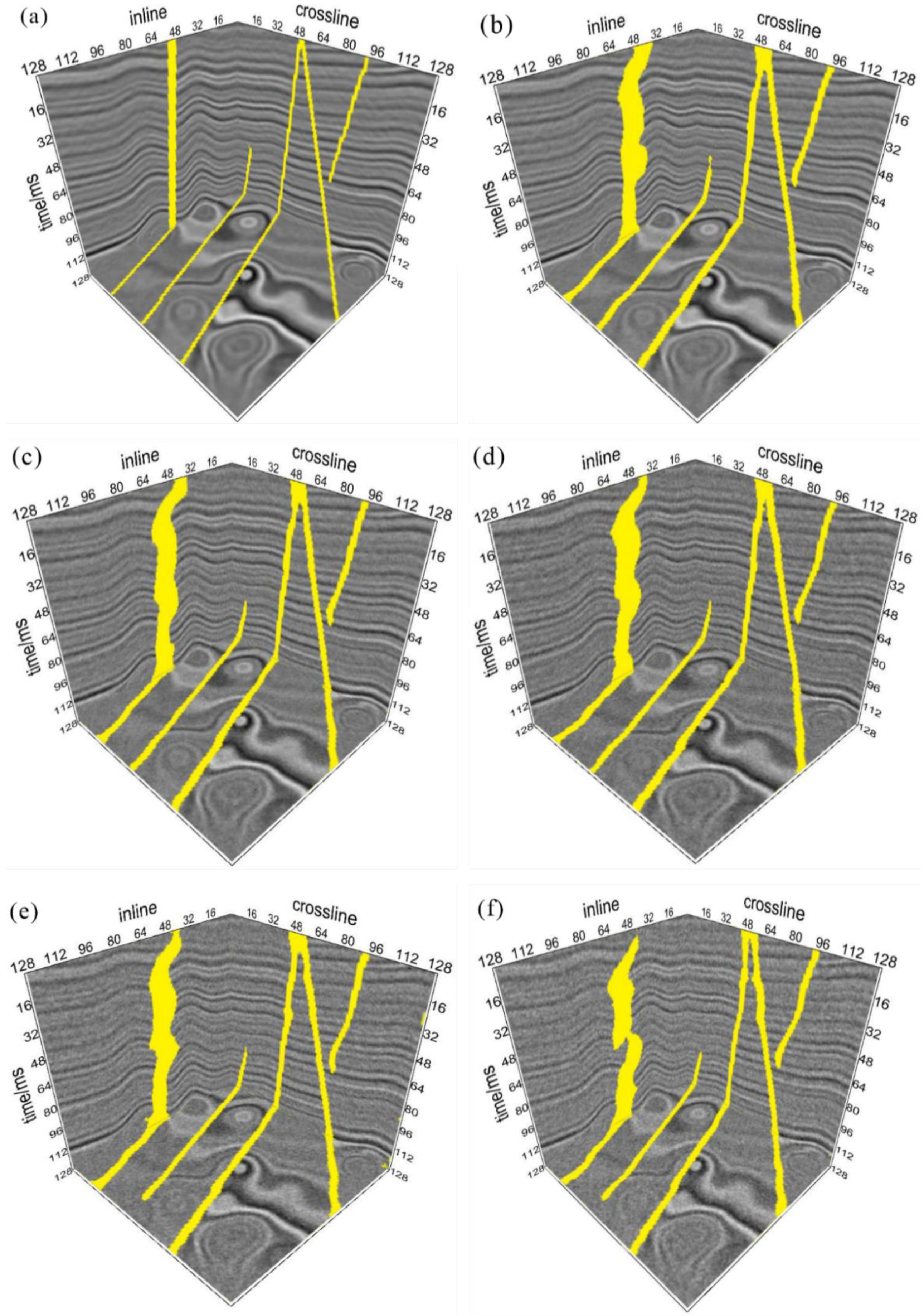
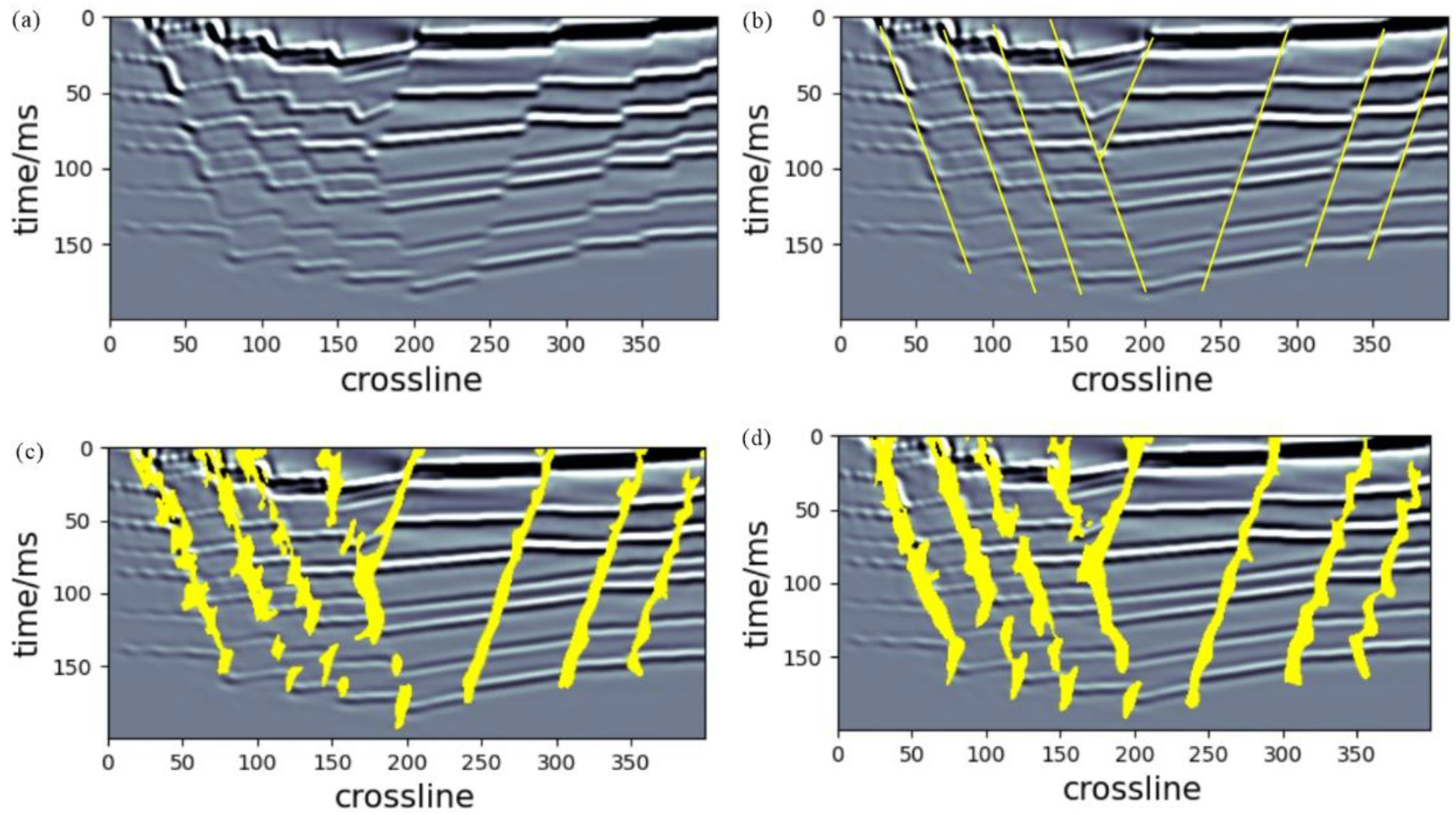
To validate the generalization ability of the SE-UNet model, the network model obtained from the network training in this study was applied to publicly available Netherlands F3 3D seismic data acquired offshore in the North Sea, with well-developed regional faults and large data volumes. Therefore, this study intercepted a part of the application: the selected data crossline ranged from 100 to 611, inline ranged from 300 to 683, time slice ranged from 1337 to 1848 ms, and the sampling interval was 4 ms. The prediction results were data-cleaned, and the threshold value of the fault probability was set higher than 0.7 for comparison with the UNet model. Figure 12a–d shows the 3D display of the real data and the results of the manually interpreted faults, the UNet network model recognizing the real data, and the network model recognizing the real data, respectively. The locations marked in yellow in Figure 12b are large faults and the locations marked in red are low-grade faults. Comparing Figure 12c,d shows that the SE-UNet model can accurately recognize the location of high-grade and low-grade faults, that the recognized faults were more continuous, and that more faults could be recognized in the inline. A detailed comparison with UNet is given in Section 5.
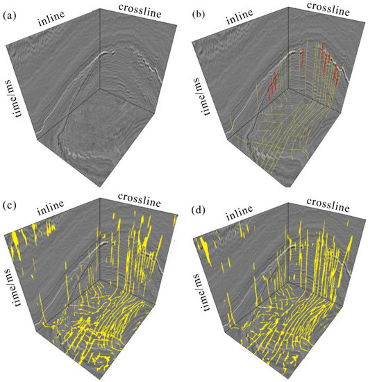
Figure 12.
Fault prediction results of real data. (a) Real seismic data; (b) manual interpretation of fault results; (c) UNet recognition; (d) SE-UNet recognition.
5. Discussion
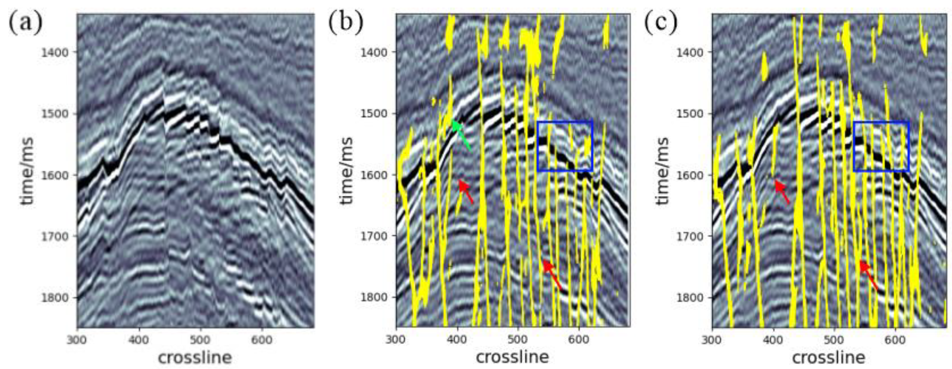
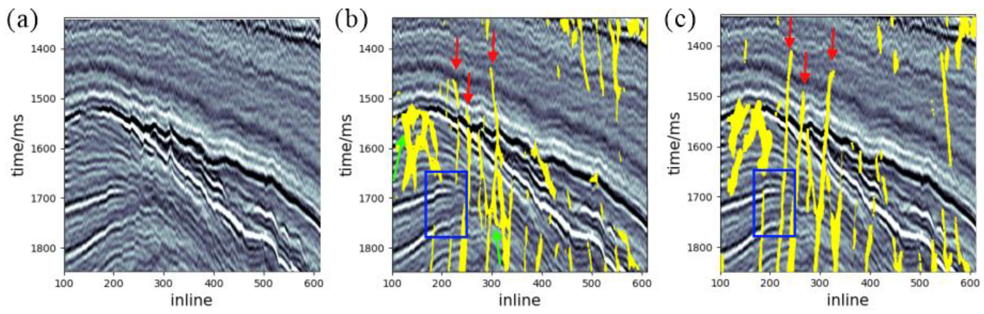
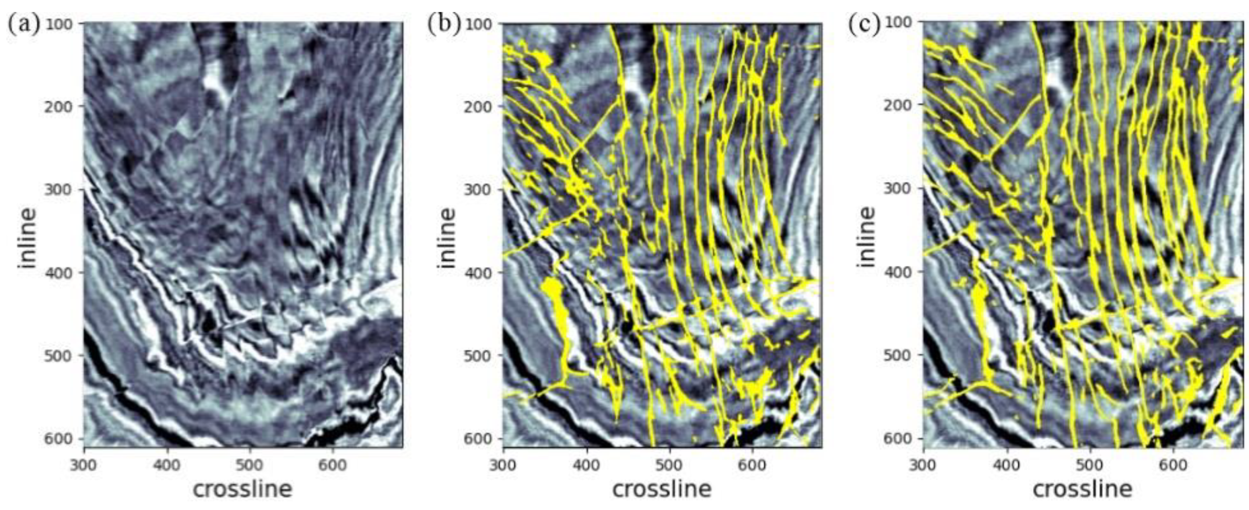
The main contribution of this study is that we constructed the SE-UNet structure that can efficiently allocate attention resources based on the codec network structure. In Section 3.4, we quantitatively analyzed the SE-UNet and UNet networks according to the evaluation criteria, and concluded that the SE-UNet network has more advantages. In this section, we discuss the identification results of SE-UNet and UNet, comparing the application effects of the two models on real data in three directions, as shown in Figure 13, Figure 14 and Figure 15. Figure 13a shows the seismic profile of the Inline200 with obvious characteristics of high-grade and low-grade faults. Figure 13b,c shows the recognition effects of the UNet and SE-UNet models, respectively. The locations indicated by the red arrows in Figure 13b,c are invisibility low-grade faults, in which the UNet model failed to recognize the results and they appeared to be missed, but the network model in this study was able to correctly recognize them. The positions indicated by green arrows in Figure 13b are continuous in the seismic event, and the UNet model misrecognized them as faults. The faults at the positions of the blue boxes in Figure 13b,c had obvious characteristics, and the prediction results of the network model in this study had better continuity compared with the UNet. Figure 14a shows the profile of the Crossline400, and Figure 14b,c shows the prediction results of the UNet and network models in this study, respectively. The location is indicated by the green arrow in Figure 14b, where the UNet model misrecognized and predicted non-faults as faults. The section tendency of the upper part of the position indicated by the red arrow in Figure 14b does not match the overall section tendency, the UNet model appeared to be confusingly recognized, and the section tendency of this position in Figure 14c was correctly predicted. Comparing the positions of the blue boxes in Figure 14b, c, the fault results predicted by the network model in this study had better continuity. Figure 15 shows the plan view of the time slice of 1437 ms and the prediction results of the two models. In the time slice direction, the prediction results of the two network models were similar, and both had suitable continuity. Overall, compared with UNet, SE-UNet could reduce the phenomenon of fault misprediction and missed prediction, the continuity of fault prediction results was better, and the recognition of low-grade faults was more advantageous.
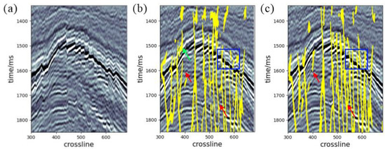
Figure 13.
Inline200 profile fault prediction results. (a) Seismic profile of Inline200; (b) prediction results of Unlet model; (c) prediction results of SE-UNet model.
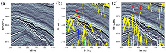
Figure 14.
Fault prediction results of Crossline400 longitudinal survey line. (a) Seismic profile of Crossline400; (b) prediction results of UNet model; (c) prediction results of SE-UNet model.

Figure 15.
The 1437 ms time slice fault prediction results. (a) Time slice; (b) prediction results of UNet model; (c) prediction results of SE-UNet model.
6. Conclusions
Traditional low-grade recognition methods are time-consuming and inaccurate. To solve these problems, we constructed an SE-UNet, which consists of four parts: an encoder, decoder, skip connection, and SE module. The encoder extracts the feature information of the training data, the skip connection preserves the information lost in the data during down-sampling, the decoder serves to recover the resolution of the data, and the SE module can select the more vital features from ample feature information through self-learning and assign higher weights to them, which improves the expressiveness of the network. The 500 pairs of simulated seismic data and the corresponding fault labels were generated by Wu’s method, and the network model was trained, validated, and trialed. Finally, the network model was applied to the real data with high recognition results. The following insights were gleaned in this work.
(1) Fault recognition with SE-UNet network can effectively achieve the recognition of low-grade faults. The test accuracy of the network model was improved to 95.23% and the recall of the test data was improved to 97.31%. The recognition efficiency was also significantly improved, as it took only 20 s to recognize data with dimensions of 128 × 384 × 512. Compared with UNet, SE-UNet can recognize faults more accurately and effectively, and the fault continuity is higher, particularly in the recognition of low-grade faults.
(2) The sample set in this paper is the simulated data, and there are some differences from the real data. In future research, real data and labels can be added to the sample library to improve the authenticity and diversity of the sample set.
(3) In the application of real working area, the real data contain some features that the network has not learned, which leads to misrecognition or missing recognition. In future research, unsupervised transfer learning can be used to input the real data into the network as the target domain to achieve more accurate prediction of the real data.
Author Contributions
Conceptualization, R.D. and D.W.; methodology, Y.Z.; software, M.C. and T.H.; writing—original draft preparation, Y.Z.; writing—review and editing, R.D., D.W., L.Z., J.Y. and S.Z.; visualization, Y.Z. All authors have read and agreed to the published version of the manuscript.
Funding
This research was funded by the: Natural Science Foundation of Shandong Province, grant number ZR202103050722; Major Research Plan on West-Pacific Earth System Multispheric Interactions, grant number 92058213; National Natural Science Foundation of China grant number 41676039 and 41930535.
Data Availability Statement
Not applicable.
Conflicts of Interest
The authors declare no conflict of interest.
References
- Xu, Y. Interpretation of seismic profile faults. China Pet. Chem. Stand. Qual. 2012, 33, 50. [Google Scholar]
- Carter, N.; Lines, L. Fault imaging using edge detection and coherency measures on Hibernia 3-D seismic data. Lead. Edge 2001, 20, 64–69. [Google Scholar] [CrossRef]
- Bi, C.; Sun, Y.; Zhou, H. Application of C3 coherence in fault identification of Ningbo tectonic belt. Inn. Mong. Petrochem. Ind. 2015, 41, 125–129. [Google Scholar]
- Li, Q. Application of variance cube technology in the interpretation of small faults in Zhuanlongwan coal mine. Shaanxi Coal 2019, 38, 122–124+130. [Google Scholar]
- He, H.; Wang, Q.; Cheng, H. Multi-scale Edge Detection Technology in Identifying Lower-order Faults. J. Oil Gas Technol. 2010, 32, 226–228+431. [Google Scholar]
- Ma, Y.; Su, C.; Zhang, J.; Liu, J. Low-order fault structure-oriented Canny property edge detection and recognition method. Geophys. Geochem. Explor. 2020, 44, 698–703. [Google Scholar]
- Pedersen, S.; Skov, T.; Randen, T.; Sønneland, L. Automatic Fault Extraction Using Artificial Ants. In SEG Technical Program Expanded Abstracts 2002; Society of Exploration Geophysicists: Houston, TX, USA, 2002. [Google Scholar]
- Zhang, X.; Li, T.; Shi, Y.; Zhao, Y. The Application of Fracture Interpretation Technology Based on Ant Tracking in Sudeerte Oilfield. Acta Geol. Sin. Engl. Ed. 2015, 89, 437–438. [Google Scholar] [CrossRef]
- Chen, X.; Yang, W.; He, Z.; Zhong, W.; Wen, X. The algorithm of 3D multi-scale volumetric curvature and its application. Appl. Geophys. 2012, 9, 65–72. [Google Scholar] [CrossRef]
- Lodhi, H. Computational biology perspective: Kernel methods and deep learning. Wiley Interdiscip. Rev. Comput. Stat. 2012, 4, 455–465. [Google Scholar] [CrossRef]
- Zhou, S.; Chen, Q.; Wang, X. Active deep learning method for semi-supervised sentiment classification. Neurocomputing 2013, 120, 536–546. [Google Scholar] [CrossRef]
- Brosch, T.; Tam, R. Manifold Learning of Brain MRIs by Deep Learning. In Medical Image Computing and Computer-Assisted Intervention (MICCAI); Spring: Berlin/Heidelberg, Germany, 2013. [Google Scholar]
- Mangos, P.; Noël, A.; Hulse. Advances in machine learning applications for scenario intelligence: Deep learning. In Theoretical Issues in Ergonomics Science; Taylor & Francis: London, UK, 2017; Volume 18. [Google Scholar]
- Yang, J.; Ding, R.; Lin, N.; Zhao, L.; Zhao, S.; Zhang, Y.; Zhang, J. Research progress of intelligent identification of seismic faults based on deep learning. Prog. Geophys. 2022, 37, 298–311. [Google Scholar]
- Tang, S.; Wang, Z. Semantic Segmentation of Street Scenes Based on Double Attention Mechanism. Comput. Mod. 2021, 10, 69–74. [Google Scholar]
- Shang, J.; Liu, Y.; Gao, X. Semantic segmentation of road scene based on multi-scale feature extraction. Comput. Appl. Softw. 2021, 38, 174–178. [Google Scholar]
- Liu, J.; Zhang, Y.; Tang, L.; Zhen, Y. Lane Line Detection and Fitting Method Based on Semantic Segmentation Results. Automob. Appl. Technol. 2022, 47, 30–33. [Google Scholar]
- Taghanaki, S.; Abhishek, K.; Cohen, J.; Cohen-Adad, J.; Hamarneh, G. Deep Semantic Segmentation of Natural and Medical Images: A Review. Artif. Intell. Rev. 2020, 54, prepublish. [Google Scholar] [CrossRef]
- Li, H.; Iwamoto, Y.; Han, X. An Efficient and Accurate 3D Multiple-Contextual Semantic Segmentation Network for Medical Volumetric Images. In Proceedings of the 2021 43rd Annual International Conference of the IEEE Engineering in Medicine and Biology Society, Piscataway, NJ, USA, 1–5 November 2021. [Google Scholar]
- Ai, C.; Song, Y.; Lv, Q. Research on a medical image semantic segmentation algorithm based on deep learning. Basic Clin. Pharmacol. Toxicol. 2021, 128, 184. [Google Scholar]
- Wang, X.; Li, Z.; Lyu, Y. Medical image segmentation based on multi⁃scale context⁃aware and semantic adaptor. J. Jilin Univ. Eng. Technol. Ed. 2022, 52, 640–647. [Google Scholar] [CrossRef]
- Yu, T. Based on the improved fast iris localization of semantic segmentation model. Mod. Comput. 2020, 15, 121–125. [Google Scholar]
- Wang, C.; Sun, Z. A Benchmark for Iris Segmentation. J. Comput. Res. Dev. 2020, 57, 395–412. [Google Scholar]
- Zhou, R.; Shen, W. PI-Unet: Research on Precise Iris Segmentation Neural Network Model for Heterogeneous Iris. Comput. Eng. Appl. 2021, 57, 223–229. [Google Scholar]
- Wu, X.; Liang, L.; Shi, Y.; Fomel, S. FaultSeg3D: Using synthetic data sets to train an end-to-end convolutional neural network for 3D seismic fault segmentation. Geophysics 2019, 84, IM35–IM45. [Google Scholar] [CrossRef]
- Wu, J.; He, S.; Yang, Q.; Guo, A.; Wu, J. Research on low-order fault identification method based on fully Convolutional Neural Network (FCN). In Proceedings of the SPG/SEG Nanjing 2020 International Geophysical Conference, Nanjing, China, 13–16 September 2020. [Google Scholar]
- Liu, Z.; He, X.; Zhang, Z.; Zhou, Q.; Zhang, S. Low-order fault identification technique based on 3D U-NET full Convolution Neural Network(CNN). Prog. Geophys. 2021, 36, 2519–2530. (In Chinese) [Google Scholar]
- Yang, J.; Chen, S. U-net with residual module is applied to fault detection. In Proceedings of the SPG/SEG Nanjing 2020 International Geophysical Conference, Nanjing, China, 13–16 September 2020. [Google Scholar]
- Chang, D.; Yong, X.; Wang, Y.; Yang, W.; Li, H.; Zhang, G. Seismic fault interpretation based on deep convolutional neural networks. Oil Geophys. Prospect. 2021, 56, 1–8. [Google Scholar]
- Feng, C.; Pan, J.; Li, C.; Yao, Q.; Liu, J. Fault high-resolution recognition method based on deep neural network. Earth Sci. 2020, 1–15. [Google Scholar] [CrossRef]
- Zhang, H. Research on Desert Seismic Random Noise Suppression Based on Convolutional Autoencoder Neural Network with Attention Module; Jilin University: Jilin, China, 2021. [Google Scholar]
- Yang, C.; Zhou, Y.; He, H.; Cui, T.; Wang, Y. Global context and attention-based deep convolutional neural network for seismic data denoising. Geophys. Prospect. Pet. 2021, 60, 751–762+855. [Google Scholar]
- Han, L.; Chai, Z.; Song, L.; Liu, X.; Fu, C. Reverse Time Migration Compensation Method of Seismic Wave Based on Deep Learning. Well Logging Technol. 2022, 46, 109–113. [Google Scholar]
- Zhang, M. A multiple suppression method based on self-attention convolution auto-encoder. Geophys. Prospect. Pet. 2022, 61, 454–462. [Google Scholar]
- Hu, J.; Shen, L.; Albanie, S.; Sun, G.; Wu, E. Squeeze-and-Excitation Networks. In Proceedings of the IEEE Transactions on Pattern Analysis and Machine Intelligence, Salt Lake City, UT, USA, 18–23 June 2018. [Google Scholar]
- Wu, X.; Geng, Z.; Shi, Y.; Pham, N.; Fomel, S.; Caumon, G. Building realistic structure models to train convolutional neural networks for seismic structural interpretation. Geophysics 2019, 85, 4745–4750. [Google Scholar]
- Luo, Q.; Huang, H.; Wang, B. Genetic types of low-grade faults and their geologic significance. Pet. Geol. Recovery Effic. 2007, 19–21+25+112. [Google Scholar] [CrossRef]


Publisher’s Note: MDPI stays neutral with regard to jurisdictional claims in published maps and institutional affiliations. |
© 2022 by the authors. Licensee MDPI, Basel, Switzerland. This article is an open access article distributed under the terms and conditions of the Creative Commons Attribution (CC BY) license (https://creativecommons.org/licenses/by/4.0/).