
Stochastic Wind Power Generation Planning in Liberalised Electricity Markets within a Heterogeneous Landscape


Abstract
1. Introduction
1.1. Motivation
Research Question: Taking generation stochasticity and optimal operational decisions in a geographically heterogeneous landscape into account, how can policy-makers make optimal decisions about the trade-off between system cost and GHG emissions with respect to their preferences?
1.2. Related Literature
1.3. Contribution and Organisation
- developing a stochastic bilevel optimisation model for a multi-nodal GEP problem, taking into account the heterogeneity in the suitability for the generation of renewable energy of different locations;
- conjointly optimising the policy decision on the introduction of an emissions-reduction regulation and the investment decisions into different generation assets to increase societal efficiency;
- explicitly accounting for operational decisions in a heterogeneous stochastic landscape with a (potentially) high penetration of RES;
- recasting the multi-objective problem into a single objective to be able to find convergent optima instead of using heuristic search, given the social planner’s preferences on GHG emissions;
- applying our model to a realistic use case, relying on real world data combined with a Monte Carlo scenario generation and -reduction approach to draw conclusions on its implications for the real world.
2. Methods
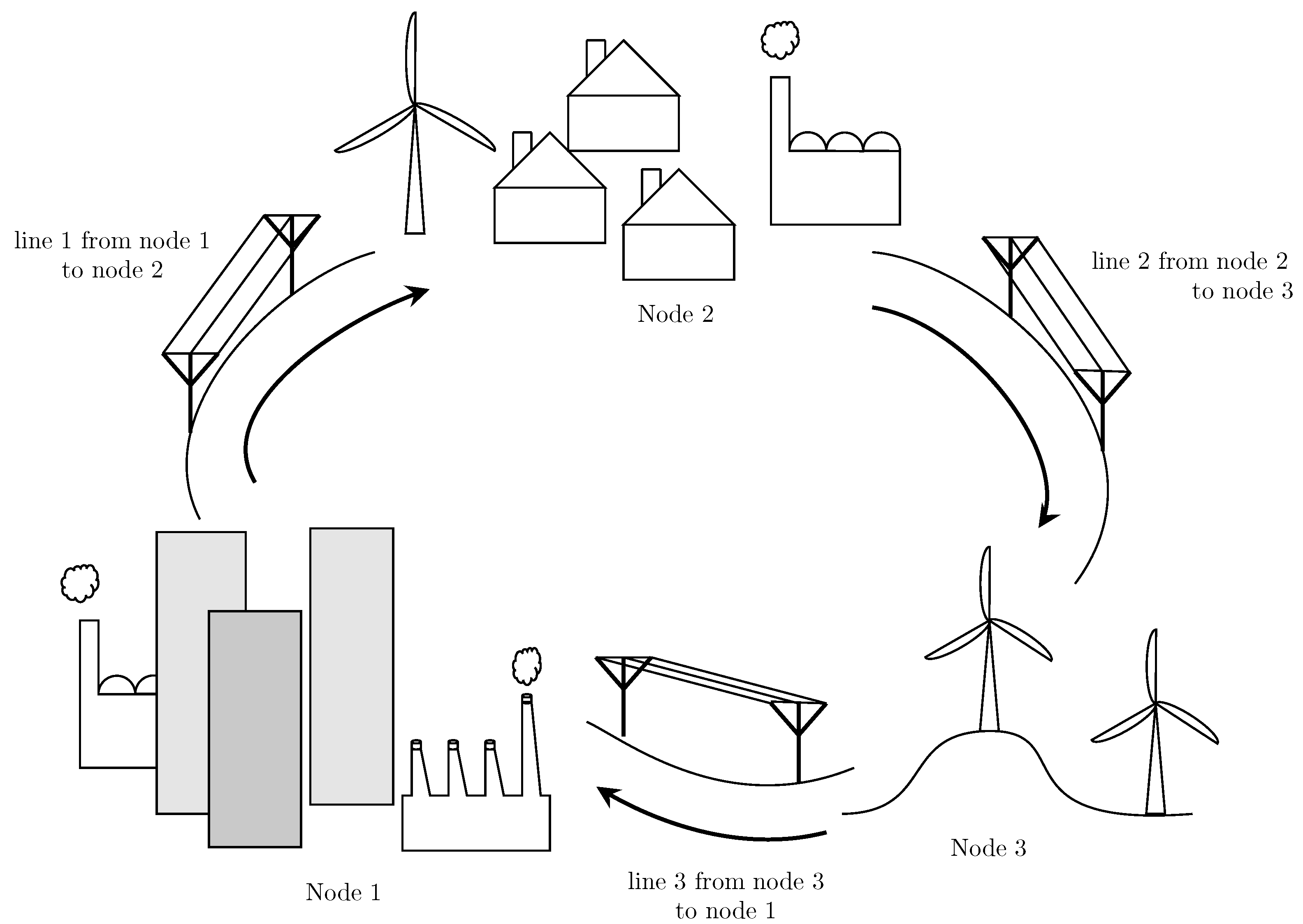
2.1. Problem Statement
2.2. Problem Formulation
2.2.1. Multi-Objective Formulation
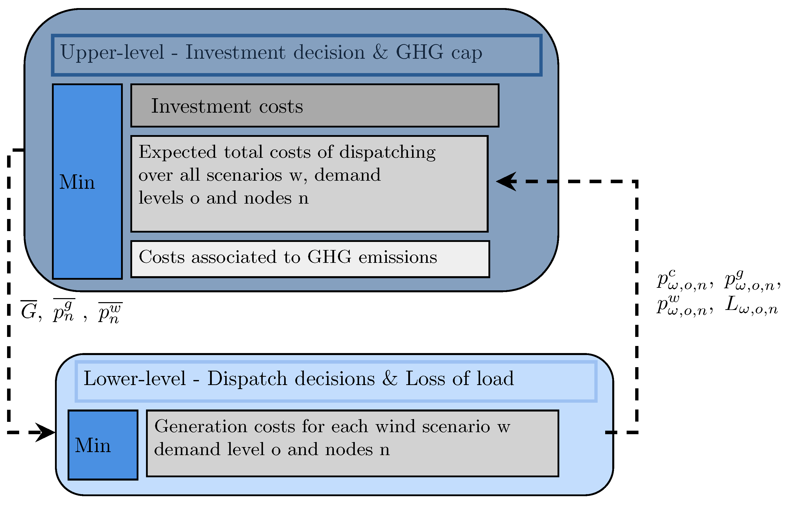
2.2.2. Bilevel Formulation
2.3. Solution Strategy
3. Numerical Experiment
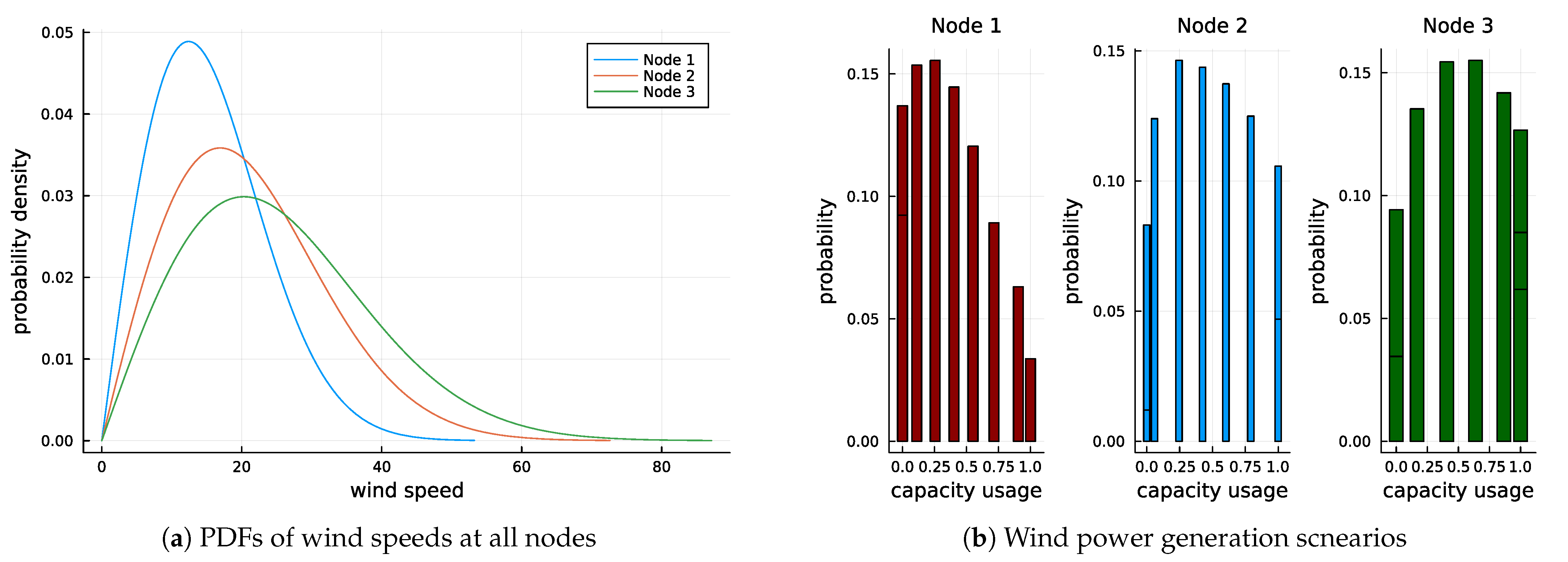
3.1. Assumptions
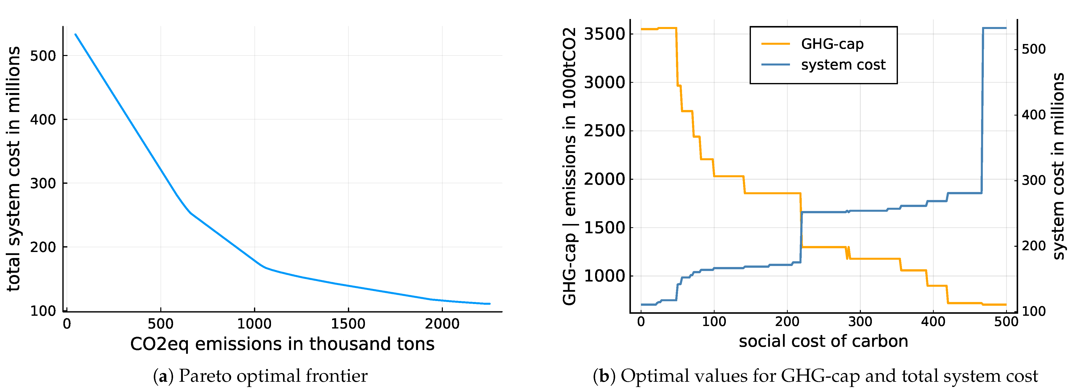
3.2. Results
4. Discussion
5. Conclusions
Author Contributions
Funding
Data Availability Statement
Acknowledgments
Conflicts of Interest
Nomenclature
| Variable | Description | Variable | Description |
| Indices: | UL decision variable: | ||
| o | Demand level | Wind power capacity expansion at node n | |
| Wind scenario | |||
| n | Node | Gas power capacity expansion at node n | |
| a | Asset | Investment option (binary) is set to 1 for the optimal investment option | |
| q | investment decision | Emissions cap | |
| l | Line | ||
| LL decision variable: | |||
| Parameters: | Amount of power supplied by coal | ||
| Social cost of carbon per unit of CO2eq emission | Amount of power supplied by gas | ||
| Annualised investment costs per MW of wind capacity installed | Amount of power supplied by wind | ||
| Annualised investment costs per MW of gas capacity installed | Loss of load | ||
| Investment of size q in asset class a at nodes n | Power flow through transmission line coming from node n | ||
| Hours per year in operating condition o | Power flow through transmission line running to node n | ||
| Probability of wind power scenario | Power flow through line l | ||
| Unit costs of power supplied by coal | Voltage angle at sending node | ||
| Unit costs of power supplied by gas | Voltage angle at receiving node | ||
| Cost associated with one unit of lost load | |||
| Emissions associated with one unit of electrical energy produced from coal | Dual variables: | ||
| Emissions associated with one unit of electrical energy produced from gas | Marginal nodal price of generation | ||
| Flow capacity of line l | Shadow price of wind power capacity | ||
| Susceptance of line l | Shadow price of gas power capacity | ||
| wind conditions at in scenario at node n | Shadow price of coal power capacity | ||
| load demand at node n & demand level o | Dual variable of the emissions constraint | ||
| Dual variables of transmission constraints: | |||
| , , , , , | |||
| Auxiliary variables: | |||
| , |
Appendix A. Full Model Specification
References
- IEA. IEA CO2 Emissions from Fuel Combustion Statistics: Greenhouse Gas Emissions from Energy. Available online: https://www.oecd-ilibrary.org/energy/data/iea-co2-emissions-from-fuel-combustion-statistics_co2-data-en (accessed on 21 September 2022).
- IPCC. Climate Change 2022: Mitigation of Climate Change. Contribution of Working Group III to the Sixth Assessment Report of the Intergovernmental Panel on Climate Change; Technical Report; IPCC: Cambridge, UK; New York, NY, USA, 2022. [Google Scholar]
- IEA. World Energy Outlook 2021; IEA: Paris, France, 2021. [Google Scholar]
- Ekardt, F. Sustainability: Transformation, Governance, Ethics, Law, 3rd ed.; Environmental Humanities: Transformation, Governance, Ethics, Law; Springer International Publishing: Cham, Switzerland, 2020. [Google Scholar] [CrossRef]
- Stern, D.I. Energy and economic growth. In Routledge Handbook of Energy Economics, 1st ed.; Soytaş, U., Sarı, R., Eds.; Routledge: Milton Park, UK, 2019. [Google Scholar] [CrossRef]
- Khezri, R.; Mahmoudi, A. Review on the state-of-the-art multi-objective optimisation of hybrid standalone/grid-connected energy systems. IET Gener. Transm. Distrib. 2020, 14, 4285–4300. [Google Scholar] [CrossRef]
- Conejo, A.J.; Baringo Morales, L.; Kazempour, S.J.; Siddiqui, A.S. Investment in Electricity Generation and Transmission; Springer International Publishing: Cham, Switzerland, 2016. [Google Scholar] [CrossRef]
- Ning, Y.; Chen, K.; Zhang, B.; Ding, T.; Guo, F.; Zhang, M. Energy conservation and emission reduction path selection in China: A simulation based on Bi-Level multi-objective optimization model. Energy Policy 2020, 137, 111116. [Google Scholar] [CrossRef]
- Zhou, S.; Yang, J.; Yu, S. A Stochastic Multi-Objective Model for China’s Provincial Generation-Mix Planning: Considering Variable Renewable and Transmission Capacity. Energies 2022, 15, 2797. [Google Scholar] [CrossRef]
- Chen, F.; Huang, G.; Fan, Y. A linearization and parameterization approach to tri-objective linear programming problems for power generation expansion planning. Energy 2015, 87, 240–250. [Google Scholar] [CrossRef]
- Valle, A.d.; Wogrin, S.; Reneses, J. Multi-objective bi-level optimization model for the investment in gas infrastructures. Energy Strategy Rev. 2020, 30, 100492. [Google Scholar] [CrossRef]
- Aldarajee, A.H.M.; Hosseinian, S.H.; Vahidi, B.; Dehghan, S. Security constrained multi-objective bi-directional integrated electricity and natural gas co-expansion planning considering multiple uncertainties of wind energy and system demand. IET Renew. Power Gener. 2020, 14, 1395–1404. [Google Scholar] [CrossRef]
- Aghaei, J.; Akbari, M.A.; Roosta, A.; Baharvandi, A. Multiobjective generation expansion planning considering power system adequacy. Electr. Power Syst. Res. 2013, 102, 8–19. [Google Scholar] [CrossRef]
- Gong, J.W.; Li, Y.P.; Lv, J.; Huang, G.H.; Suo, C.; Gao, P.P. Development of an integrated bi-level model for China’s multi-regional energy system planning under uncertainty. Appl. Energy 2022, 308, 118299. [Google Scholar] [CrossRef]
- Yang, Y.; Luo, Z.; Yuan, X.; Lv, X.; Liu, H.; Zhen, Y.; Yang, J.; Wang, J. Bi-Level Multi-Objective Optimal Design of Integrated Energy System Under Low-Carbon Background. IEEE Access 2021, 9, 53401–53407. [Google Scholar] [CrossRef]
- Marler, R.T.; Arora, J.S. The weighted sum method for multi-objective optimization: New insights. Struct. Multidiscip. Optim. 2010, 41, 853–862. [Google Scholar] [CrossRef]
- Oree, V.; Sayed Hassen, S.Z.; Fleming, P.J. Generation expansion planning optimisation with renewable energy integration: A review. Renew. Sustain. Energy Rev. 2017, 69, 790–803. [Google Scholar] [CrossRef]
- Asgharian, V.; Abdelaziz, M.M.A.; Kamwa, I. Multi-stage bi-level linear model for low carbon expansion planning of multi-area power systems. IET Gener. Transm. Distrib. 2019, 13, 9–20. [Google Scholar] [CrossRef]
- Asgharian, V.; Genc, V.M.I. Multi-objective optimization for voltage regulation in distribution systems with distributed generators. In Proceedings of the 2016 IEEE Electrical Power and Energy Conference (EPEC), Ottawa, ON, Canada, 12–14 October 2016; IEEE: New York, NY, USA, 2016; pp. 1–6. [Google Scholar] [CrossRef]
- Hussain, A.; Kim, H.M. Goal-Programming-Based Multi-Objective Optimization in Off-Grid Microgrids. Sustainability 2020, 12, 8119. [Google Scholar] [CrossRef]
- Gorenstin, B.; Campodonico, N.; Costa, J.; Pereira, M. Power system expansion planning under uncertainty. IEEE Trans. Power Syst. 1993, 8, 129–136. [Google Scholar] [CrossRef]
- Hu, Y. An NSGA-II based multi-objective optimization for combined gas and electricity network expansion planning. Appl. Energy 2016, 167, 280–293. [Google Scholar] [CrossRef]
- Park, H.; Baldick, R. Stochastic Generation Capacity Expansion Planning Reducing Greenhouse Gas Emissions. IEEE Trans. Power Syst. 2015, 30, 1026–1034. [Google Scholar] [CrossRef]
- Home-Ortiz, J.M.; Melgar-Dominguez, O.D.; Pourakbari-Kasmaei, M.; Mantovani, J.R.S. A stochastic mixed-integer convex programming model for long-term distribution system expansion planning considering greenhouse gas emission mitigation. Int. J. Electr. Power Energy Syst. 2019, 108, 86–95. [Google Scholar] [CrossRef]
- Conejo, A.J.; Nogales, F.; Arroyo, J. Price-taker bidding strategy under price uncertainty. IEEE Trans. Power Syst. 2002, 17, 1081–1088. [Google Scholar] [CrossRef]
- Mitridati, L.; Pinson, P. A Bayesian Inference Approach to Unveil Supply Curves in Electricity Markets. IEEE Trans. Power Syst. 2018, 33, 2610–2620. [Google Scholar] [CrossRef]
- Fitiwi, D.Z.; Lynch, M.; Bertsch, V. Enhanced network effects and stochastic modelling in generation expansion planning: Insights from an insular power system. Socio-Econ. Plan. Sci. 2020, 71, 100859. [Google Scholar] [CrossRef]
- Zolfaghari Moghaddam, S. Generation and transmission expansion planning with high penetration of wind farms considering spatial distribution of wind speed. Int. J. Electr. Power Energy Syst. 2019, 106, 232–241. [Google Scholar] [CrossRef]
- Hemmati, R.; Hooshmand, R.A.; Khodabakhshian, A. Coordinated generation and transmission expansion planning in deregulated electricity market considering wind farms. Renew. Energy 2016, 85, 620–630. [Google Scholar] [CrossRef]
- Colson, B.; Marcotte, P.; Savard, G. An overview of bilevel optimization. Ann. Oper. Res. 2007, 153, 235–256. [Google Scholar] [CrossRef]
- Kazempour, S.J.; Conejo, A.J. Strategic Generation Investment Under Uncertainty Via Benders Decomposition. IEEE Trans. Power Syst. 2012, 27, 424–432. [Google Scholar] [CrossRef]
- Garces, L.; Conejo, A.J.; Garcia-Bertrand, R.; Romero, R. A Bilevel Approach to Transmission Expansion Planning Within a Market Environment. IEEE Trans. Power Syst. 2009, 24, 1513–1522. [Google Scholar] [CrossRef]
- Li, R.; Wang, W.; Chen, Z.; Wu, X. Optimal planning of energy storage system in active distribution system based on fuzzy multi-objective bi-level optimization. J. Mod. Power Syst. Clean Energy 2018, 6, 342–355. [Google Scholar] [CrossRef]
- Ghaderi, A.; Parsa Moghaddam, M.; Sheikh-El-Eslami, M. Energy efficiency resource modeling in generation expansion planning. Energy 2014, 68, 529–537. [Google Scholar] [CrossRef]
- Acemoglu, D.; Aghion, P.; Bursztyn, L.; Hemous, D. The Environment and Directed Technical Change. Am. Econ. Rev. 2012, 102, 131–166. [Google Scholar] [CrossRef]
- Acemoglu, D.; Akcigit, U.; Hanley, D.; Kerr, W. Transition to Clean Technology. J. Political Econ. 2016, 124, 52–104. [Google Scholar] [CrossRef]
- Rockström, J.; Gaffney, O.; Rogelj, J.; Meinshausen, M.; Nakicenovic, N.; Schellnhuber, H.J. A roadmap for rapid decarbonization. Science 2017, 355, 1269–1271. [Google Scholar] [CrossRef]
- Geels, F.W.; Sovacool, B.K.; Schwanen, T.; Sorrell, S. Sociotechnical transitions for deep decarbonization. Science 2017, 357, 1242–1244. [Google Scholar] [CrossRef] [PubMed]
- Qazi, A.; Hussain, F.; Rahim, N.A.; Hardaker, G.; Alghazzawi, D.; Shaban, K.; Haruna, K. Towards Sustainable Energy: A Systematic Review of Renewable Energy Sources, Technologies, and Public Opinions. IEEE Access 2019, 7, 63837–63851. [Google Scholar] [CrossRef]
- Stehly, T.; Beiter, P.; Duffy, P. 2019 Cost of Wind Energy Review; Technical Report; National Renewable Energy Laboratory: Golden, CO, USA, 2020.
- Wang, P.; Deng, X.; Zhou, H.; Yu, S. Estimates of the social cost of carbon: A review based on meta-analysis. J. Clean. Prod. 2019, 209, 1494–1507. [Google Scholar] [CrossRef]
- Carrion, M.; Arroyo, J.; Conejo, A. A Bilevel Stochastic Programming Approach for Retailer Futures Market Trading. IEEE Trans. Power Syst. 2009, 24, 1446–1456. [Google Scholar] [CrossRef]
- Talari, S.; Shafie-khah, M.; Wang, F.; Aghaei, J.; Catalao, J.P.S. Optimal Scheduling of Demand Response in Pre-Emptive Markets Based on Stochastic Bilevel Programming Method. IEEE Trans. Ind. Electron. 2017, 66, 1453–1464. [Google Scholar] [CrossRef]
- Li, Y.; Zio, E. Uncertainty analysis of the adequacy assessment model of a distributed generation system. Renew. Energy 2012, 41, 235–244. [Google Scholar] [CrossRef]
- Talari, S.; Yazdaninejad, M.; Haghifam, M. Stochastic-based scheduling of the microgrid operation including wind turbines, photovoltaic cells, energy storages and responsive loads. IET Gener. Transm. Distrib. 2015, 9, 1498–1509. [Google Scholar] [CrossRef]
- EIA. Frequently Asked Questions (FAQs)—U.S. Energy Information Administration (EIA). Available online: https://www.eia.gov/tools/faqs/faq.php (accessed on 29 September 2022).
- EIA. Average Operating Heat Rate for Selected Energy Sources. Available online: https://www.eia.gov/electricity/annual/html/epa_08_01.html (accessed on 29 September 2022).
- EIA. U.S. Natural Gas Prices. Available online: https://www.eia.gov/dnav/ng/ng_pri_sum_dcu_nus_m.htm (accessed on 29 September 2022).
- EIA. Electricity Monthly Update—U.S. Energy Information Administration (EIA). Available online: https://www.eia.gov/electricity/monthly/update/print-version.php (accessed on 29 September 2022).
- Office of Energy Efficiency & Renewable Energy. How Do Wind Turbines Survive Severe Storms? Available online: https://www.energy.gov/eere/articles/how-do-wind-turbines-survive-severe-storms (accessed on 29 September 2022).
- Office of Energy Efficiency & Renewable Energy. Wind Turbines: The Bigger, the Better. Available online: https://www.energy.gov/eere/articles/wind-turbines-bigger-better (accessed on 29 September 2022).
- Project, S.E.E. Wyoming Energy Fact Sheet. Available online: https://www.swenergy.org/Data/Sites/1/media/documents/publications/factsheets/WY-Factsheet.pdf (accessed on 29 September 2022).
- EIA. Cost and Performance Characteristics of New Generating Technologies, Annual Energy Outlook 2022. Available online: https://www.eia.gov/outlooks/aeo/assumptions/pdf/table_8.2.pdf (accessed on 4 September 2022).
- Spath, P.L.; Mann, M.K. Life Cycle Assessment of a Natural Gas Combined Cycle Power Generation System; Technical Report; NREL: Cole Boulevard, CO, USA, 2000. [CrossRef]
- Fridays for Future. Unsere Forderungen an Die Politik|Fridays for Future. Available online: https://fridaysforfuture.de/forderungen/ (accessed on 30 September 2022).
- Resources for the Future. Social Cost of Carbon Explorer. Available online: https://www.rff.org/publications/data-tools/scc-explorer/ (accessed on 30 September 2022).
- Nguyen, H.T.; Felder, F.A. Generation expansion planning with renewable energy credit markets: A bilevel programming approach. Appl. Energy 2020, 276, 115472. [Google Scholar] [CrossRef]
- Cheng, Y.; Zhang, N.; Kang, C. Bi-Level Expansion Planning of Multiple Energy Systems under Carbon Emission Constraints. In Proceedings of the 2018 IEEE Power & Energy Society General Meeting (PESGM), Portland, OR, USA, 5–10 August 2018; IEEE: New York, NY, USA, 2018; pp. 1–5. [Google Scholar] [CrossRef]


| Source | Multiobjective | Stochastic | Bilevel |
|---|---|---|---|
| [9] | Emissions, Cost, Revenue | RES Generation | |
| [13] | Emissions, Cost, Reliability | Peak Load Surplus | |
| [22] | Infrastructure Cost, Operation Cost, Emissions | Wind | |
| [12] | Cost, Voltage Stability | Load, Wind | |
| [8] | Emissions, GDP, Energy Consumption | National/Regional Level | |
| [11] | Demand Utility, Cost | Investment, Operation | |
| [33] | Cost load Shaving, Volatility, Reserve Capability | Investment, Operation | |
| [34] | Investment, Operation | ||
| [18] | Wind | Area-Coordination | |
| [29] | Wind | ||
| [27] | Multiple | ||
| [23] | Load, Wind | ||
| [24] | Load, Wind | ||
| [28] | Load, Wind | ||
| [10] | Emissions, Cost, Generation | ||
| [14] | Emissions, Cost | Load | Emissions-Cost-trade-off |
| [15] | Emissions, Cost | Load | Cost-Emissions-trade-off |
| This Study | Emissions, Cost | Wind | Investment, Operation |
| Node 1 | Node 2 | Node 3 | |
|---|---|---|---|
| max additional wind cap. in MW | 120 | 540 | 840 |
| max additional gas cap. in MW | 200 | 400 | 200 |
| base load in MWh | 219 | 53 | 11 |
| medium load in MWh | 328 | 79 | 17 |
| peak load in MWh | 437 | 105 | 22 |
| average wind speed in Mph | 11 | 15 | 18 |
| Wind | Coal | Natural Gas | |
|---|---|---|---|
| annualised investment cost per MW in $US | 10,000 | — | 28,000 |
| minimum unit increment in capacity expansion | 60 MW | — | 50 MW |
| variable cost in | 0 | ≈29 | ≈58 |
| CO2eq emissions in | 0 | ≈1 | ≈0.41 |
Publisher’s Note: MDPI stays neutral with regard to jurisdictional claims in published maps and institutional affiliations. |
© 2022 by the authors. Licensee MDPI, Basel, Switzerland. This article is an open access article distributed under the terms and conditions of the Creative Commons Attribution (CC BY) license (https://creativecommons.org/licenses/by/4.0/).
Share and Cite
Sund, L.; Talari, S.; Ketter, W. Stochastic Wind Power Generation Planning in Liberalised Electricity Markets within a Heterogeneous Landscape. Energies 2022, 15, 8109. https://doi.org/10.3390/en15218109
Sund L, Talari S, Ketter W. Stochastic Wind Power Generation Planning in Liberalised Electricity Markets within a Heterogeneous Landscape. Energies. 2022; 15(21):8109. https://doi.org/10.3390/en15218109
Chicago/Turabian StyleSund, Lennard, Saber Talari, and Wolfgang Ketter. 2022. "Stochastic Wind Power Generation Planning in Liberalised Electricity Markets within a Heterogeneous Landscape" Energies 15, no. 21: 8109. https://doi.org/10.3390/en15218109
APA StyleSund, L., Talari, S., & Ketter, W. (2022). Stochastic Wind Power Generation Planning in Liberalised Electricity Markets within a Heterogeneous Landscape. Energies, 15(21), 8109. https://doi.org/10.3390/en15218109