Article

Eliminate Time Dispersion of Seismic Wavefield Simulation with Semi-Supervised Deep Learning

1
State Key Laboratory of Petroleum Resources and Prospecting, China University of Petroleum (Beijing), Beijing 102249, China
2
Unconventional Petroleum Research Institute, China University of Petroleum (Beijing), Beijing 102249, China
3
College of Geophysics, China University of Petroleum (Beijing), Beijing 102249, China
*
Author to whom correspondence should be addressed.
Energies 2022, 15(20), 7701; https://doi.org/10.3390/en15207701
Submission received: 9 September 2022 / Revised: 6 October 2022 / Accepted: 11 October 2022 / Published: 18 October 2022

Abstract

:
Finite-difference methods are the most widely used methods for seismic wavefield simulation. However, numerical dispersion is the main issue hindering accurate simulation. In the case where the finite-difference scheme is known, the time dispersion can be predicted mathematically and, thus, can be eliminated. However, when only pre-compiled software is available for wavefield simulation, which is common in practical applications, the software-used algorithm becomes a black box (unknown). Therefore, it is challenging to obtain the mathematical expression of the time dispersion, resulting in difficulty in eliminating the time dispersion. To solve this problem, we propose to use deep learning methods to eliminate time dispersion. We design a semi-supervised framework based on convolutional and recurrent neural networks for eliminating time dispersion caused by seismic wave modeling. The framework of our proposed neural network includes two main modules: Inverse Model and Forward Model, both of which have learnable parameters. The Inverse Model is used for eliminating time dispersion while the Forward Model is used for regularizing the training. Particularly, this framework includes two steps: Firstly, using the compiled modeling software to generate two data sets with large and small time steps. Secondly, we train these two modules for transformation between large time-step data (with time dispersion) and small time-step data (without time dispersion) by labeled and unlabeled data sets. In this work, the labeled data set is a paired data set with large time-step data and their corresponding small time-step data; the unlabeled data set is the large time-step data that need time-dispersion elimination. We use the unlabeled data set to guide the network. In this learning framework, re-training is required whenever the modeling algorithms, time interval, or frequency band is changed. Hence, we propose a transfer learning training method to extend from the trained model to another model, which reduces the computational cost caused by re-training. This minor drawback is offset overwhelmingly by the modeling efficiency gain with large time steps in large-scale production. Tests on two models confirm the effectiveness of the proposed method.

1. Introduction

Seismic wavefield simulation/modeling is essential for high-precision imaging of the Earth’s subsurface [1]. The conventional seismic wavefield modeling is based on the numerical solution of the wave equation. The solution of the wave equation involves the calculation of the time and space derivatives with numerical methods. Researchers have developed wave-equation-based imaging methods such as reverse-time migration [2,3] and full-waveform inversion [4,5,6]. The finite-difference (FD) scheme is the most basic and often used method to solve the wave equation [7,8,9]. However, the FD approximations of time and space derivatives lead to numerical dispersion when the sample interval is large, even if it satisfies the stable condition [10,11]. To accurately simulate the wavefield, it is possible to minimize the dispersion errors in space and time.
Researchers have proposed methods to improve finite difference spatial accuracy, including methods to lengthen the spatial difference operator and methods to optimize the spatial FD coefficients [12,13,14]. However, using long difference operators to approximate spatial partial derivatives requires more computation, and due to the saturation effect [15], the improvement of the simulation accuracy becomes small as the operator length increases. The FD coefficients of the conventional FD methods are based on the Taylor series expansion, which can only ensure the accuracy of the simulation in the low wave-number part. The optimized FD methods approximate the dispersion relation to obtaining the FD coefficients using optimized methods, such as least squares (LS) minimization [16,17,18] and simulated annealing methods [12], which can significantly improve simulation accuracy in the medium-to-high wave-number part. The pseudo-spectral (PS) methods [19,20] are used to obtain spatial partial derivatives using forward and inverse Fourier transforms. The PS methods can theoretically be accurate up to the Nyquist wave number but require more computational time than FD methods.
The time derivatives in wave equations are commonly approximated using the second-order FD format, but the low-order systems can result in significant time dispersion errors. Researchers have proposed the Lax–Wendroff methods [21,22] to improve time accuracy by replacing high-order time derivatives with spatial ones. To increase the stable time-step upper limit, optimal Lax–Wendroff methods were developed [13,23,24]. In addition, the new FD template method improves temporal accuracy by using time–space domain methods with new stencils. Liu and Sen (2013) [25] presented a centered-grid FD method with a rhombus-shaped stencil, which can achieve arbitrary even-order accuracy in the time and space domains but is computationally demanding. To balance accuracy and efficiency, Wang (2016) [18] proposed an FD method based on the combination of cross and rhombus stencils. Tang and Huang (2014) [26] developed the staggered-grid FD method of fourth- or sixth-order in time. Ren (2017) [27] presented the temporal high-order SFD schemes, and Ren (2022) [28] applied the staggered-grid FD method for source wavefield reconstruction.
Alternatively, the method of the post-propagation filter is an efficient approach to reducing time dispersion. Stork (2013) [29] firstly proposed the time dispersion correction filter, which demonstrated that time dispersion is independent of propagation path, medium, and spatial dispersion errors and successfully filtered away time dispersion errors from seismograms. Wang and Xu (2015) [30] introduced a time dispersion correction method based on the analytically anticipated time dispersion error, which improves the effectiveness of the time dispersion filter. The time dispersion filter applies the forward time-dispersion transform (FTDT) for predicting time dispersion error and the inverse time-dispersion transform (ITDT) for removal. However, the FTDT is an adjoint rather than an inverse of the ITDT, so the ITDT with their proposed filters cannot fully eliminate the time dispersion added by the FTDT. Li (2016) [31] suggested a time-varying filter to minimize time dispersion in shot recordings. Koene (2018) [32] derived the precise inverse of ITDT, which is employed as a new FTDT, where the ITDI can recover (with proper band restrictions) the input signal, and the ITDT can successfully minimize temporal dispersion of the modeling wavefields with FD, PS, and spectral element methods, enhancing temporal accuracy more effectively.
These methods are used to propagate seismic data through synthetic models, and the forward modeling methods are capable of determining the dispersion relationship quantitatively. However, because highly integrated software is typically used in practical production, software algorithms are a black box to users (i.e., it is impossible to obtain the specific forward modeling method from the compiled software) which makes it impossible to quantify the dispersion relationship of the forward modeling results, and therefore difficult to accurately eliminate the time dispersion of the modeling results. Recently, machine learning and deep learning algorithms have been utilized with some success in seismic impedance inversion [33,34], seismic modeling [35], and seismic data interpretation [36]. In this paper, we propose to use machine learning methods to overcome this problem.
The framework of our proposed neural network includes two main modules: Inverse Model and Forward Model and these two main modules for transformation between large time-step data (with time dispersion) and small time-steps data (without time dispersion). We propose a semi-supervised machine learning strategy to eliminate time dispersion. Specifically, we use deep learning to learn the mapping patterns in temporally dispersed samples. The Inverse Model is used for eliminating time dispersion while the Forward Model is used for regularizing the training. Although the deep-learning network is a “black-box”, which is difficult to be quantitatively interpreted, in this study, we can generate any amount of data that the network needs to train the network. Therefore, the network is able to perform as designed. Thus, the proposed deep-learning method is considered feasible.
The rest of this paper is organized as follows. Section 2 shows the details of our framework, which is based on semi-supervised learning to train our proposed model and then shows a new training method by transfer learning based on the pre-trained model. Section 3 provides and analyzes the experimental findings of our proposed network on the Marmousi and SEAM models. Section 4 presents discussion. Section 5 summarizes the entire paper.

2. Methods

2.1. Theory

In this work, we use a modeling program with the pseudo-spectral (PS) method as the black box, i.e., the compiled software, to generate the data set with large and small time steps. Since the PS method is used, the simulated seismic data are free of spatial dispersion but have temporal dispersion. A few training data are first generated using the modeling program with large and small time steps, which mimic the time-dispersed data and the time-dispersion-free data, respectively. The data with small time steps are used as the label of the data with large time steps.
In this paper, we propose a semi-supervised framework for eliminating time dispersion based on Convolutional Neural Networks (CNNs) and Gate Recurrent Units (GRUs). We can utilize semi-supervised networks to train not only labeled data but also unlabeled data. The unlabeled data act as constraints to better train the generative network and generate more accurate outcomes.
CNNs are used to extract feature information, where dilation convolution is used to expand the perceptual field and where the data are inputted point by point. In this work, the size of the data is large, and multiple dilation convolutions with different dilation rates are superimposed; thus, the different perceptual fields can lead to multi-scale contextual information, which also helps to reduce computational effort. Recurrent Neural Networks (RNNs) are used to extract temporal information since time dispersion data are a type of temporal data. An RNN network typically has four inputs and one output. The inputs include three gate functions—Input Gate, Forget Gate, and Output Gate—that can be used to train the network’s weights using the context-specific knowledge of the data to learn the mapping relationship between the inputs and the outputs. The GRU network is an adaptation of the RNN network that, to simplify computation, merges the typical Input Gate and Forget Gate into a single Update Gate and blends cell states with hidden states.

2.2. Network Structures

We choose two main modules for transformation between large time-step data and small time-step data: Inverse Model and Forward Model, both of which have learnable parameters; the Inverse Model is used for eliminating time dispersion, and the Forward Model is used for regularizing the training. The workflow we proposed is shown in Figure 1, which includes labeled and unlabeled data sets. The labeled data set is a paired data set with large time-step data and their corresponding small time-step data, and the unlabeled data set is large time-step data that contain time dispersion that needs to be eliminated.
The network takes input data (both labeled and unlabeled large time-step data) and feeds them to the proposed Inverse Model, which transformations the data from the source domain with time dispersion to the target domain without time dispersion, and the loss function between the label of the input and the output of the Inverse Model is minimized. Next, the generated without-time-dispersion data of the unlabeled data set is then fed into the proposed Forward Model, which converts it back to time-dispersed data, and the loss function between the original input and the output of the Forward Model is minimized. Furthermore, the network takes the other input data (labeled small time-step data) and feeds them to the proposed Forward Model, which transformations the data from the source domain without time dispersion to the target domain with time dispersion, and the loss function between the label of the input and the output of the Forward Model is minimized.
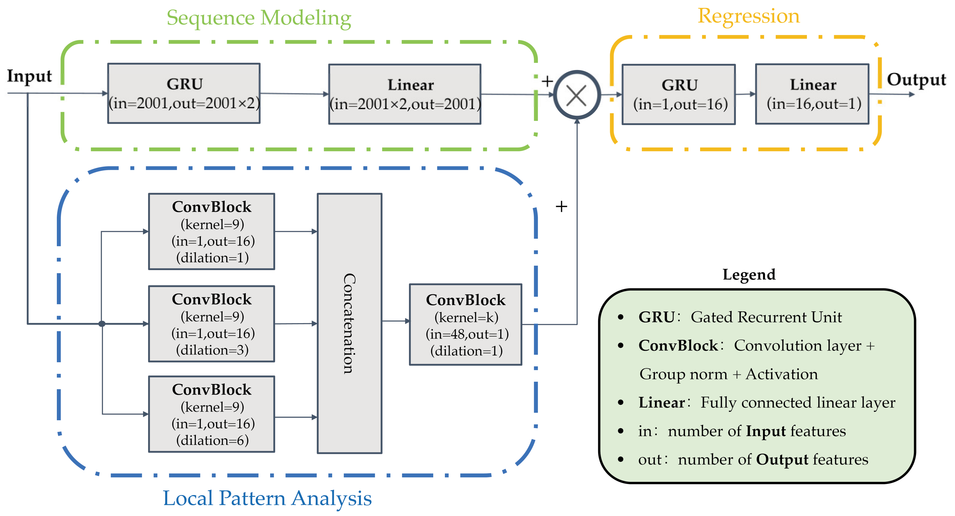
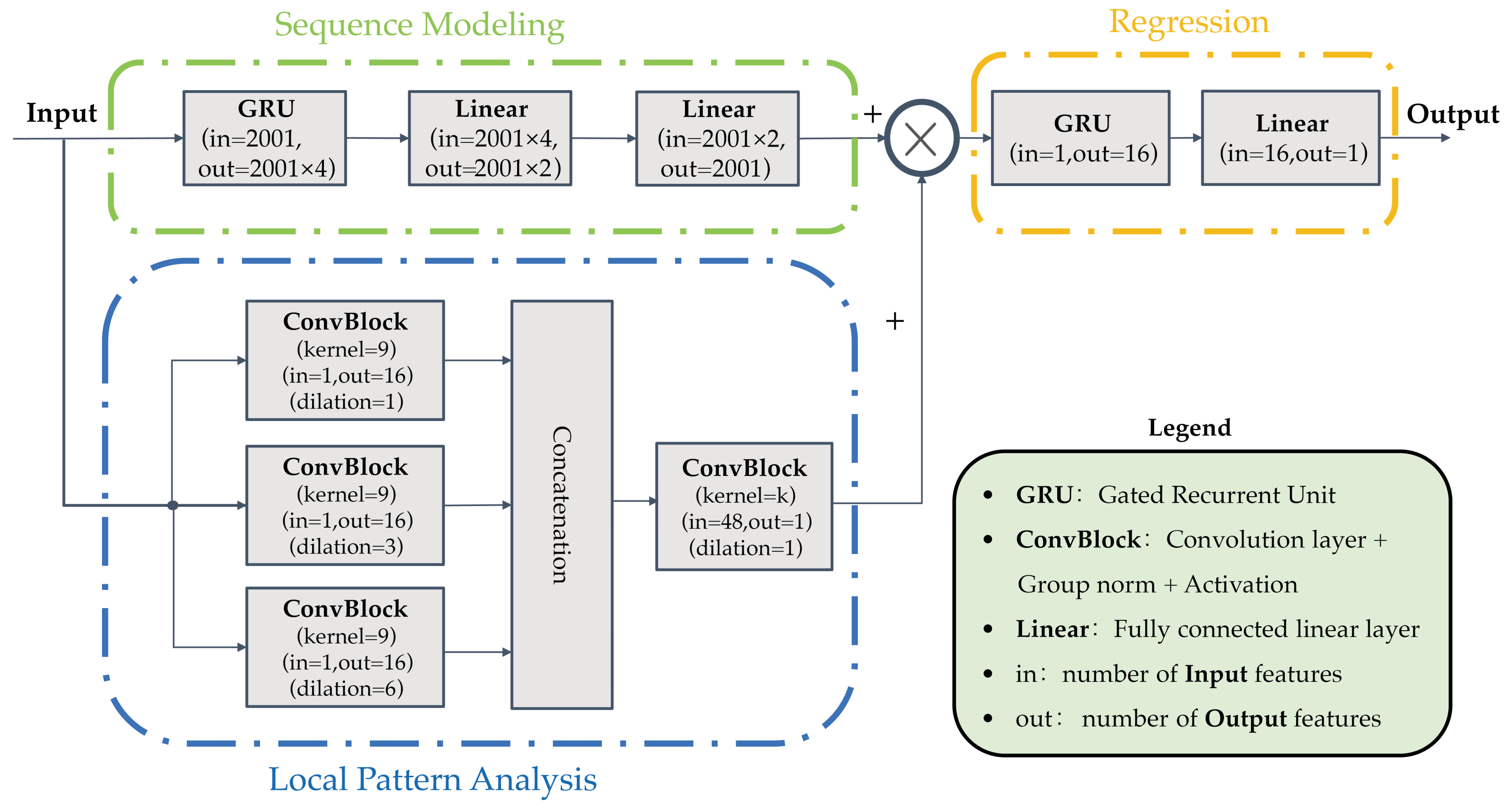
The architecture of the Inverse Model and Forward Model are similar to that used by Motaz Alfarraj [37], where the difference is the adjustment of local parameters and the removal of the upsampling submodule. Figure 2 shows the Inverse Model in the proposed workflow. The Inverse Model consists of three main submodules. These submodules are denoted as Sequence Modeling, Local Pattern Analysis, and Regression, and each have a different role in the overall model. Figure 3 shows the Forward Model architecture, which is similar to that of the Inverse Model in the proposed workflow. We noted that time-dispersion-free data need more complex mapping than time-dispersed data, so the differences are 2 times the GRU output data size and two fully-connected-layer modules in Forward Model. The fully-connected-layer modules are mainly used for compensation of resolution mismatch between input data and output data.
Sequence Modeling submodule comprises multiple Gated Recurrent Units (GRUs) [38]. The input traces of GRU are modeled as sequential data trace by trace, and temporal features are computed based on temporal variations of these data, so GRU can continually update the memory of the past and future moments and adjust its weights in the training process. Consider that more hidden layer neurons will have significantly better effects on capturing temporal features; therefore, one GRU module is set in the Sequence Modeling submodule, where we set the input data size to the number of hidden layer neurons. Then, one fully connected layer is used as a transition layer, which compensates for the dimensional mismatch between the outputs and the inputs.
Local Pattern Analysis submodule comprises three parallel 1D CNN modules, each parallel CNN module having the same convolutional kernel size and different dilation coefficients. Three outputs of these parallel CNN modules are stitched together into one output, which is then fed into another 1D CNN module with three layers and decreasing convolutional kernels. Dilation is defined as the intervals between convolution core points in the convolution layers [39]. The superposition of multiple dilated convolutions with different dilation rates expands the receptive field, and the different receptive fields lead to multi-scale temporal feature information. There is also a group normalization layer and an activation function layer between two adjacent CNN layers. The CNNs are used mainly to capture high-frequency trends in the data. The output of deep GRUs is regarded mainly as low-frequency trends in the data. To capture the frequency content of the full frequency band, the two outputs of the CNNs and GRUs are combined and fed into Regression.
The final submodule is Regression, which is used for mapping the extracted features from the other two submodules to the target data. Regression comprises a 1-layer GRU followed by a linear layer. In addition, the input layer of GRU and output layer in this submodule all use the transpose function. Hence, the output size is set to the same as the input size, i.e., one trace in and also one trace out.
In the end, we propose a transfer learning training method to extend from the trained model to another model, which helps the network adapt to new seismic data better. We consider that GRU is designed to capture the sequential relationship of input data when extracting features from the training set, and GRU continually adjusts the weights of the Local Pattern Analysis submodule. Thus, for the new seismic data, we fix the initialization of the Local Pattern Analysis submodule by using the trained model weights file and retraining the parts with the GRU. This training method can use a smaller number of training data rather than starting from scratch.

2.3. Loss Function

In this work, the input size and output size are both set to N × 1 . We denote the labeled single trace data of time-dispersed data as x, the unlabeled data as x_u, which is also the data for time-dispersion elimination. The corresponding time-dispersion-free data of x is denoted as y. The Inverse Model and Forward Model are denoted as f w I · with weights W I and f w F ( · ) with weights W F , respectively.
As shown in Figure 1, property loss 1 adds property loss 2 as property loss, which is calculated between predicted and target on traces and maps temporally dispersed data to time-dispersion-free data. Unlabeled loss is calculated between predicted and input unlabeled data. This kind of loss is adopted to constrain the prediction consistency on the dispersive time-series traces. In this part, we have modified the mean absolute error (L1) by calculating property loss and unlabeled loss separately to better fit our proposed workflow training loss function. Formally, the loss function takes the following form:
L p r o p e r t y W I , W F = 1 N L 1 f w I   x ,   y + 1 N L 1 f w F   y ,   x
L u n l a b e l e d W I , W F = 1 N L 1 ( f w F ( f w I   x u ) ,   x u )
L ( W I , W F ) = α L p r o p e r t y + β L u n l a b e l e d
The parameters of both the Inverse Model and the Forward Model are adjusted by combining both losses as in Equation (3). In this work, we choose α = 0.2 and β = 1, which are proposed by Motaz Alfarraj [37].

2.4. Training Procedure

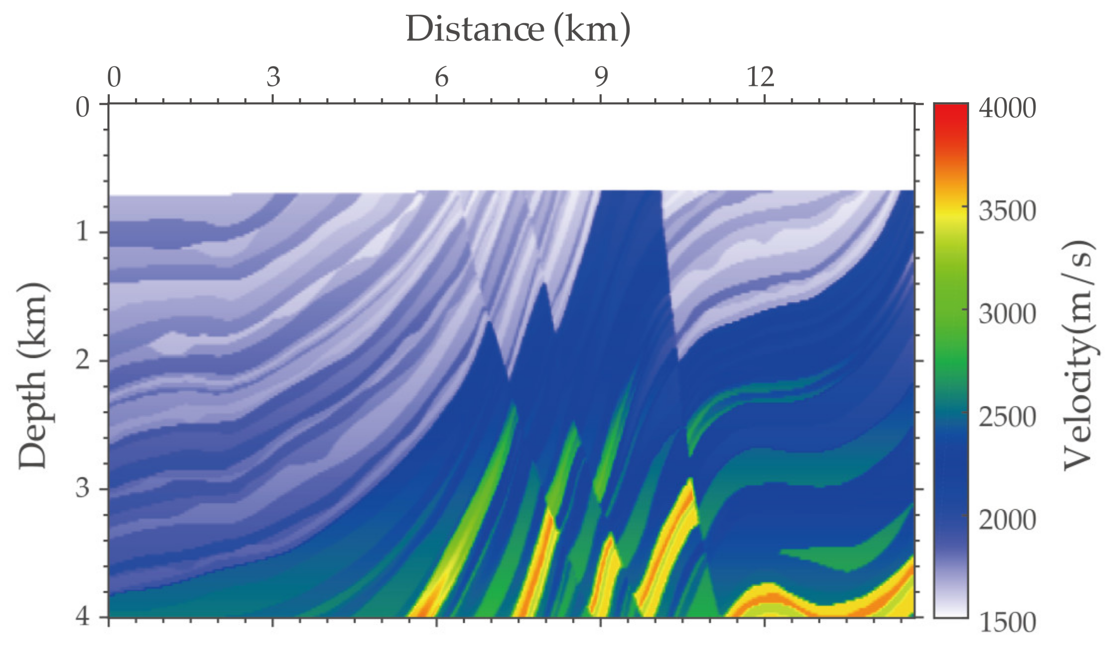
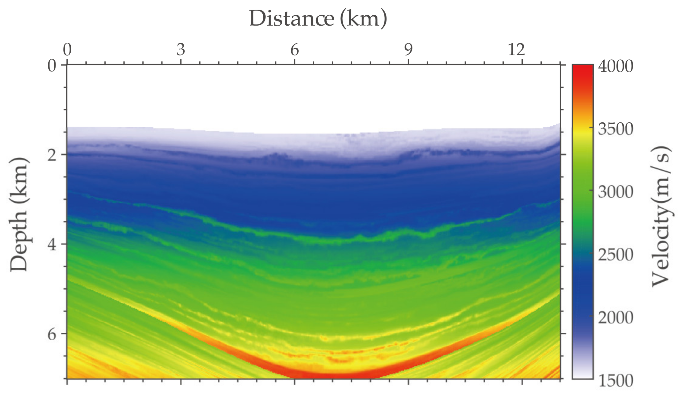
We generate the data set using a compiled wavefield modeling program, which uses the pseudo-spectral (PS) method, for simulating wavefields with large and small time steps. Firstly, the proposed strategy is tested on a partial modified Marmousi model. The corresponding velocity model is shown in Figure 4. The source wavelet is a Ricker wavelet with a dominant frequency of 15 Hz. The spatial location of the source is unequally spaced. A split-spread geometry is applied. The receiver array has a receiver spacing of 20 m. The minimum and maximum offsets are 0 m and 14,750 m, respectively. We choose the time intervals of 0.2 ms and 1.2 ms, assuming that the solution obtained with the 0.2 ms interval is time-dispersion-free data. We use approximately 90% of the shot recording data for the training set and the remainder for the test data set. The validation data are randomly picked from the test data set. Furthermore, the proposed strategy is tested on the SEAM model. The corresponding velocity model is shown in Figure 10. In the SEAM model test, we choose the time intervals of 0.4 ms and 2 ms, assuming that the solution obtained on the 0.4 ms intervals is time-dispersion-free data. Then, we apply transfer learning with the trained network from the Marmousi model and try the SEAM model with the training samples consisting of 40% of shot recording data for the training set. The training procedure for the proposed workflow is shown in Algorithm 1. The initial learning rate is 1 × 10⁻⁴, x     X represents the labeled time-dispersed data, x _ u     X _ U represents the unlabeled time-dispersed data, and y     Y represents time-dispersion-free data.
Algorithm 1 Algorithm for updating weights W I and W F .
Input: time-dispersed data sets X, X_U, time-dispersion-free data sets Y
Output: W I and W F
1: Randomly initialize parameters W I and W F
2: epoch = 500, α = 0.2, and β = 1
3: for epoch steps do
4:   for all of the labeled data sampled do
5:      X Y p r e d , Y X p r e d
6:     Calculate the Property Loss in Equation (1)
7:     Randomly sample the unlabeled data x _ u
8:      X _ U Y _ U p r e d , Y _ U p r e d X _ U p r e d
9:     Calculate the Unlabeled Loss in Equation (2)
10:    Calculate the Loss in Equation (3) using property loss, unlabeled loss, α and β
11:  end for
12:  Update W I and W F in order to minimize Loss
13: end for

3. Results

Our main goal is to eliminate time dispersion, and we apply our method to two data sets with Pytorch on a Nvidia RTX3090 GPU. Images below are mainly the results predicted on the test data sets, which are shown for evaluating the performance of the proposed workflow quantitatively.

3.1. The Data Test with the Marmousi Model

In this part, the data set is generated by using the modeling program with the velocity model of a partial modified Marmousi (Figure 4).
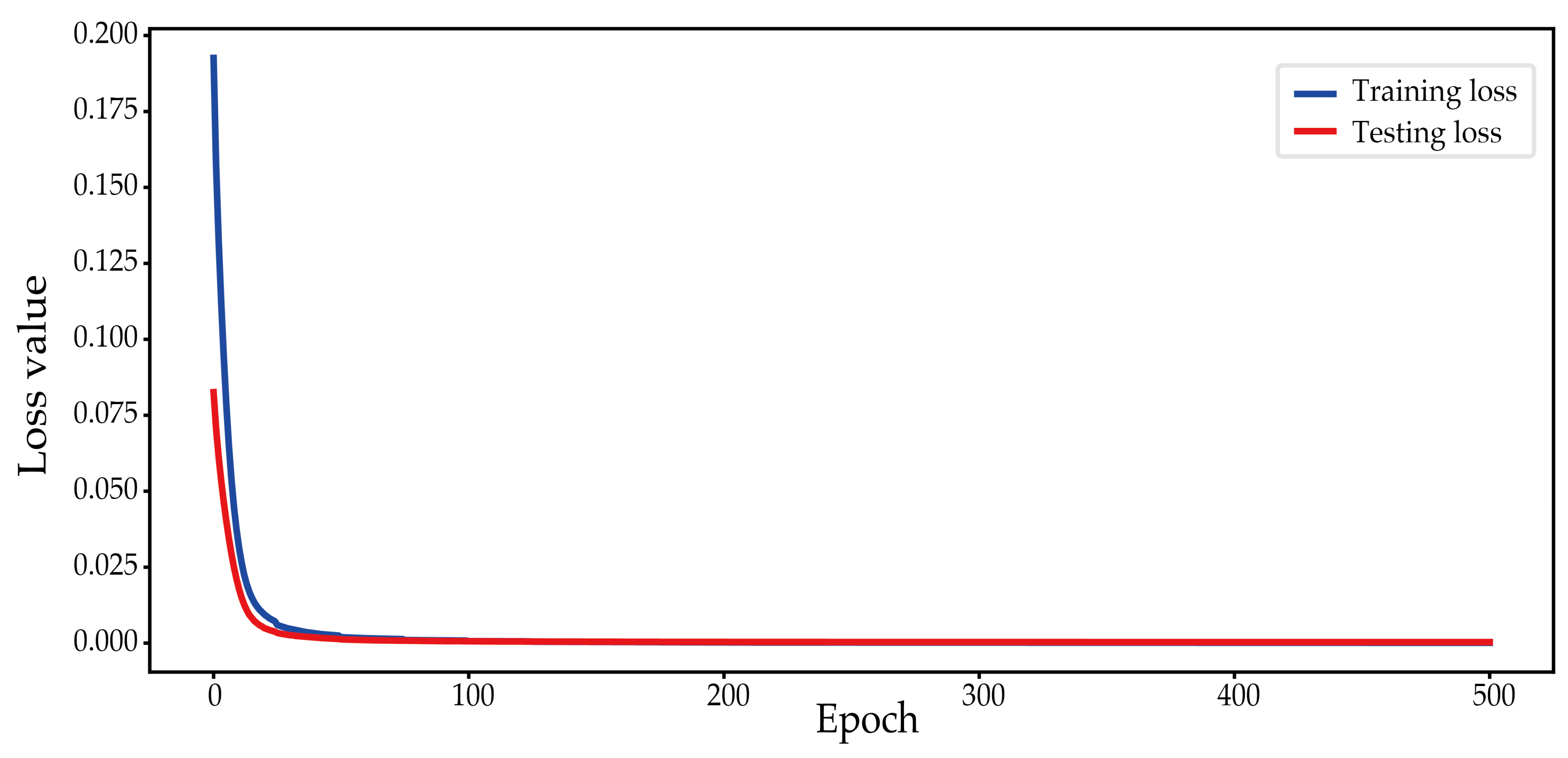
To create the data set, we choose the time intervals of 0.2 ms and 1.2 ms, assuming that the solution obtained with the 0.2 ms time intervals is approximated as time-dispersion-free data. The data set includes 32 shots, each of which contains 550 receivers with a receiver spacing of 20 m. Each trace has 2001 time sampling points by re-sampling at the time interval of 3.6 ms. We resample the data because the frequency of exploration seismic data including this example is usually less than 100 Hz. In addition, the resampling into a coarse interval can also save the computational and memory cost. In the training process, we use 30 shots, which are fed into the network sequentially trace by trace, and 2 shots for testing. Considering a sufficient amount of data and a large number of traces per shot, we set the batch size to 50. The Inverse Model and Forward Model are together trained for 500 epochs. Next, we follow the training procedure. Figure 5 shows that the loss function curve leveled off.
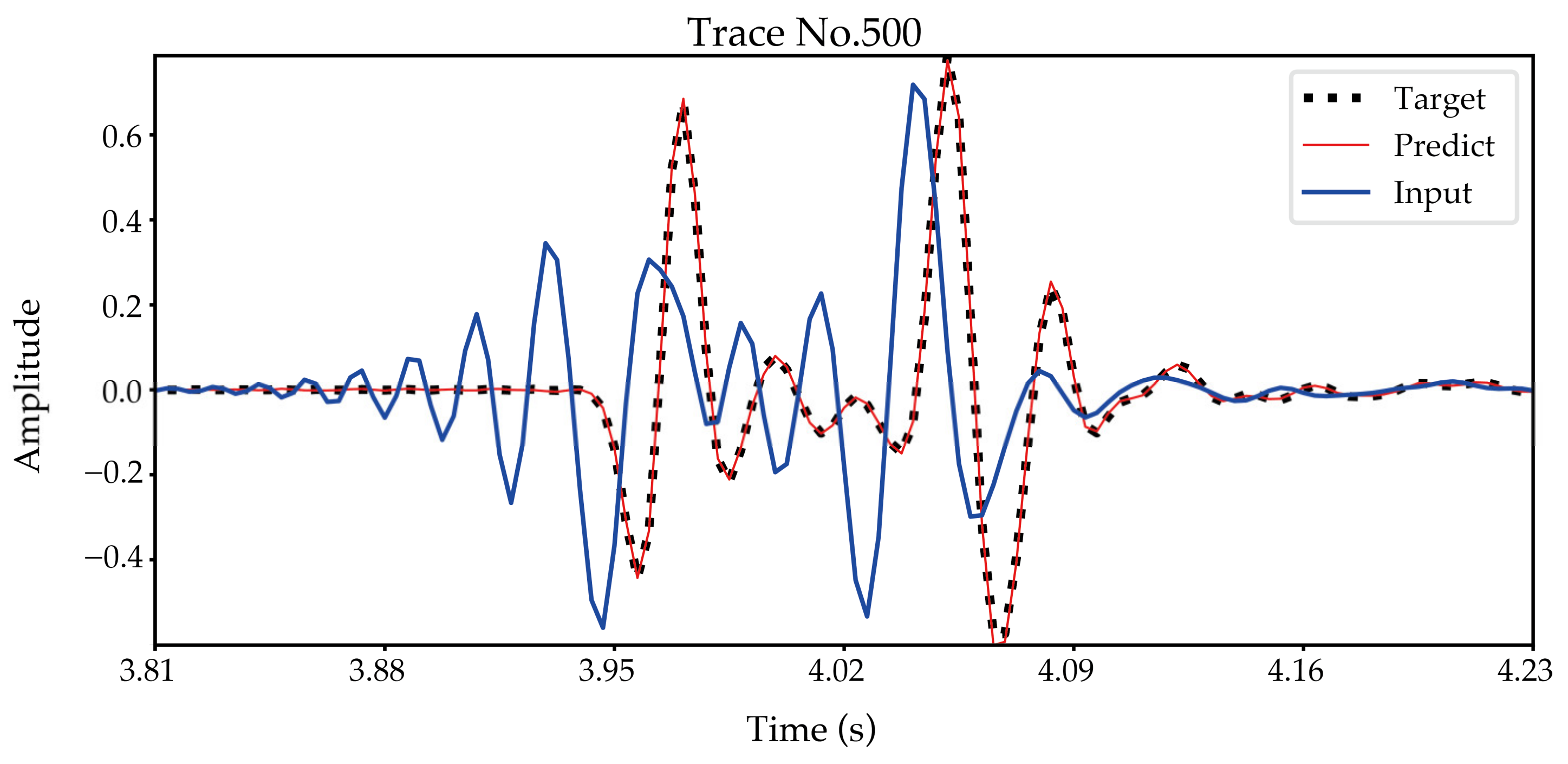
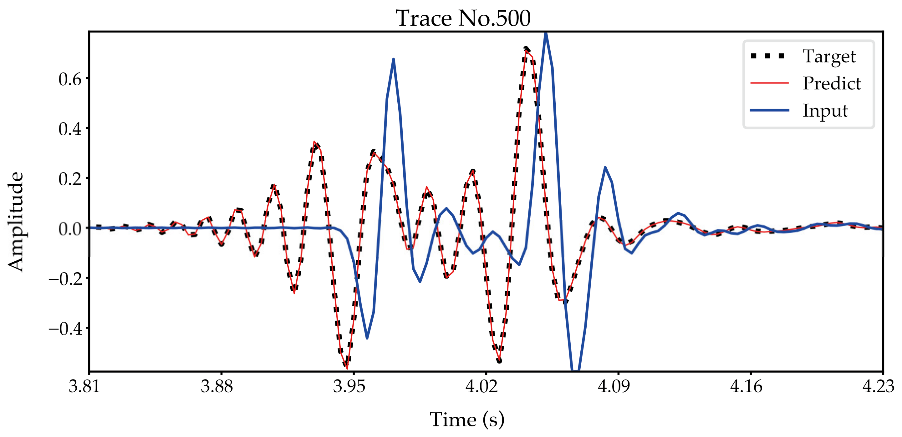
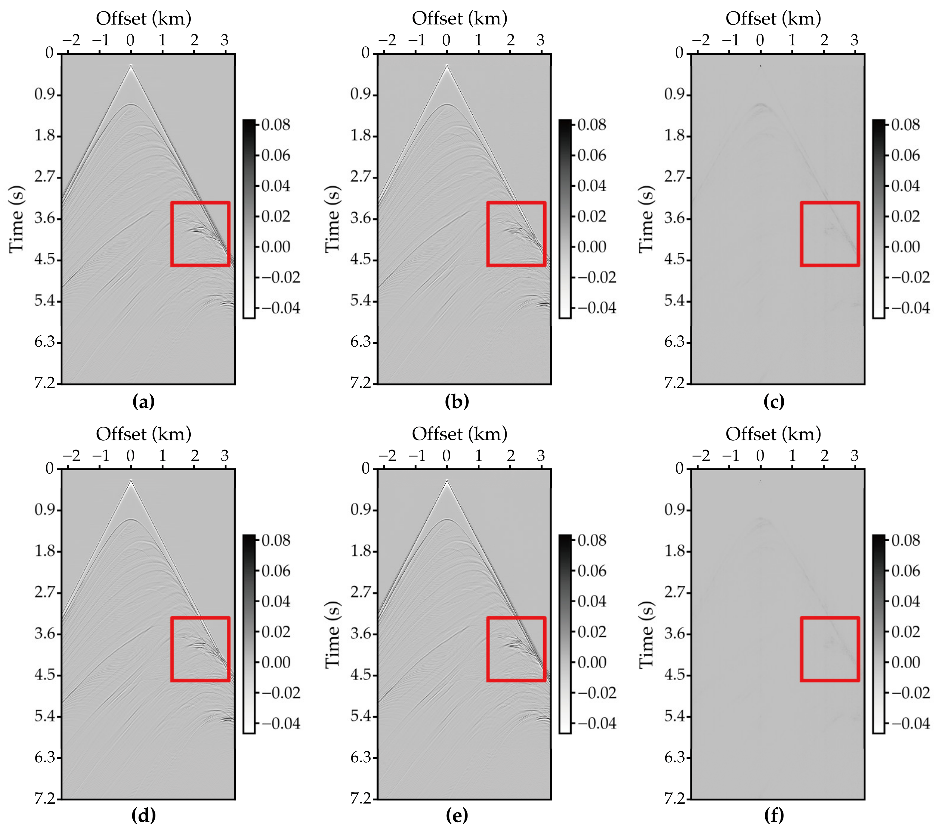
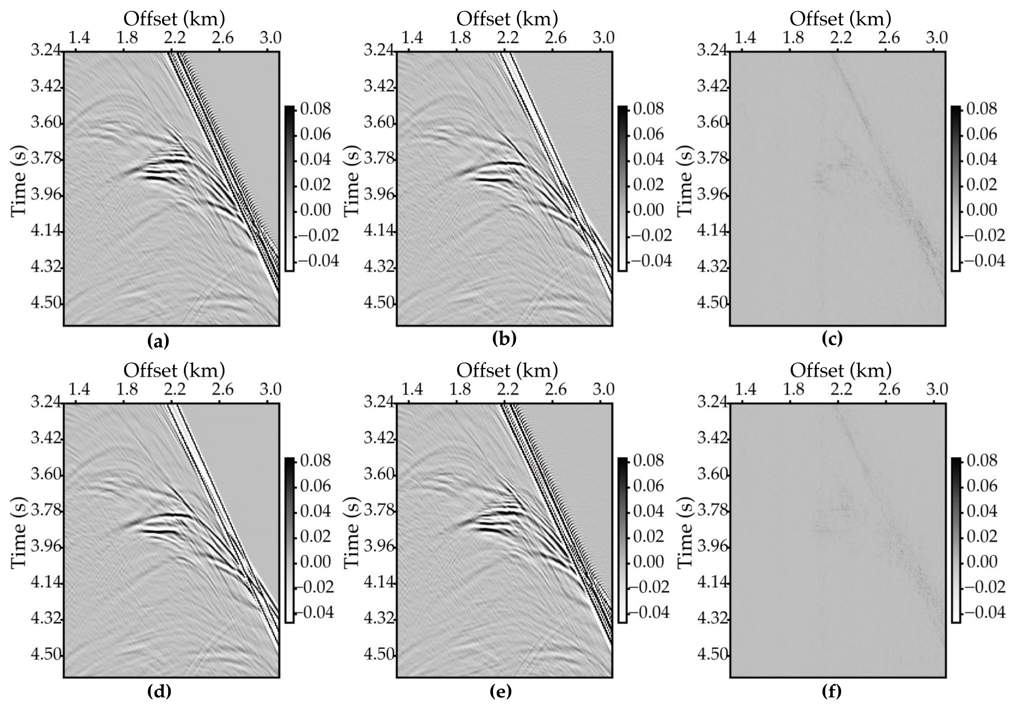
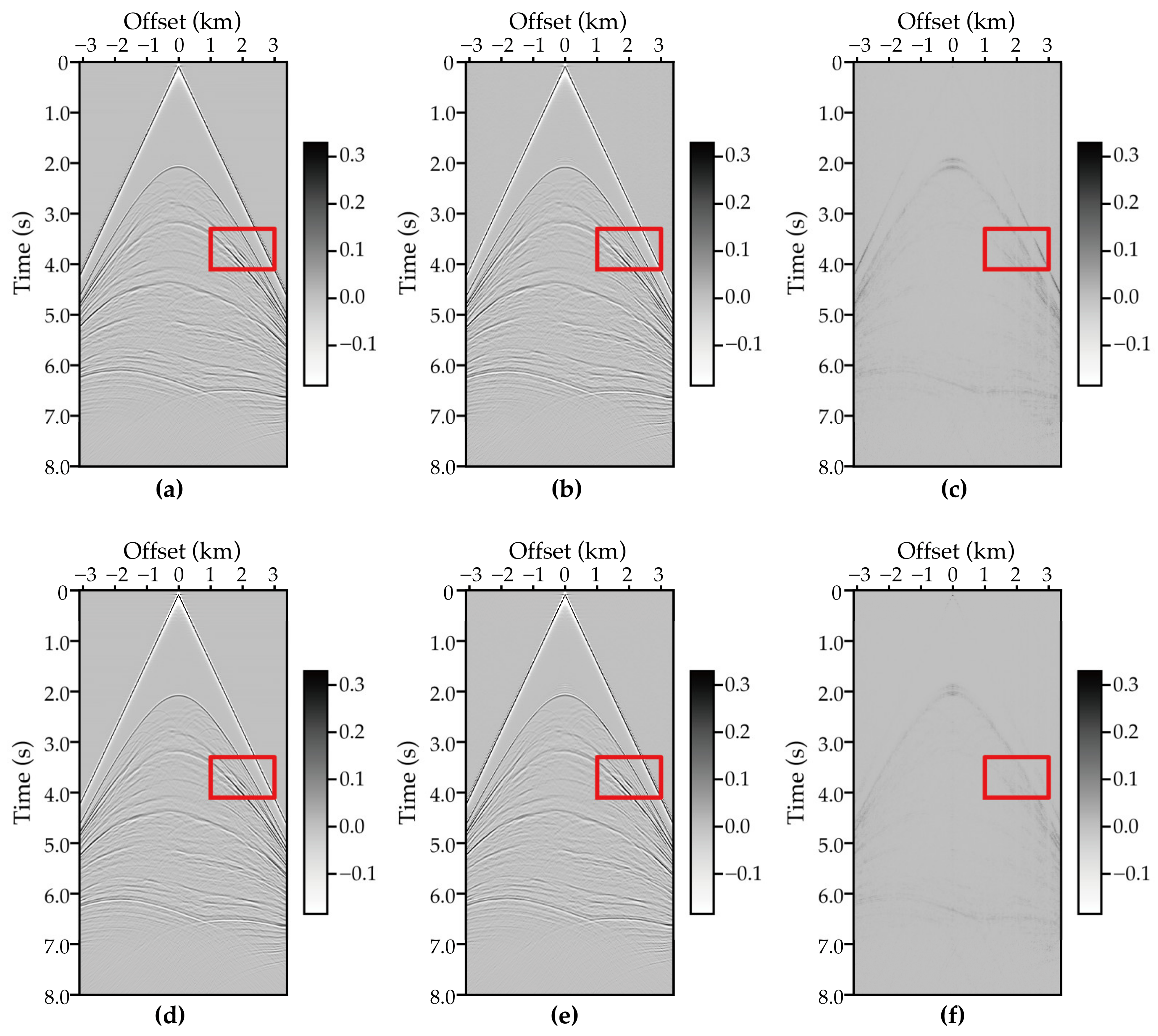
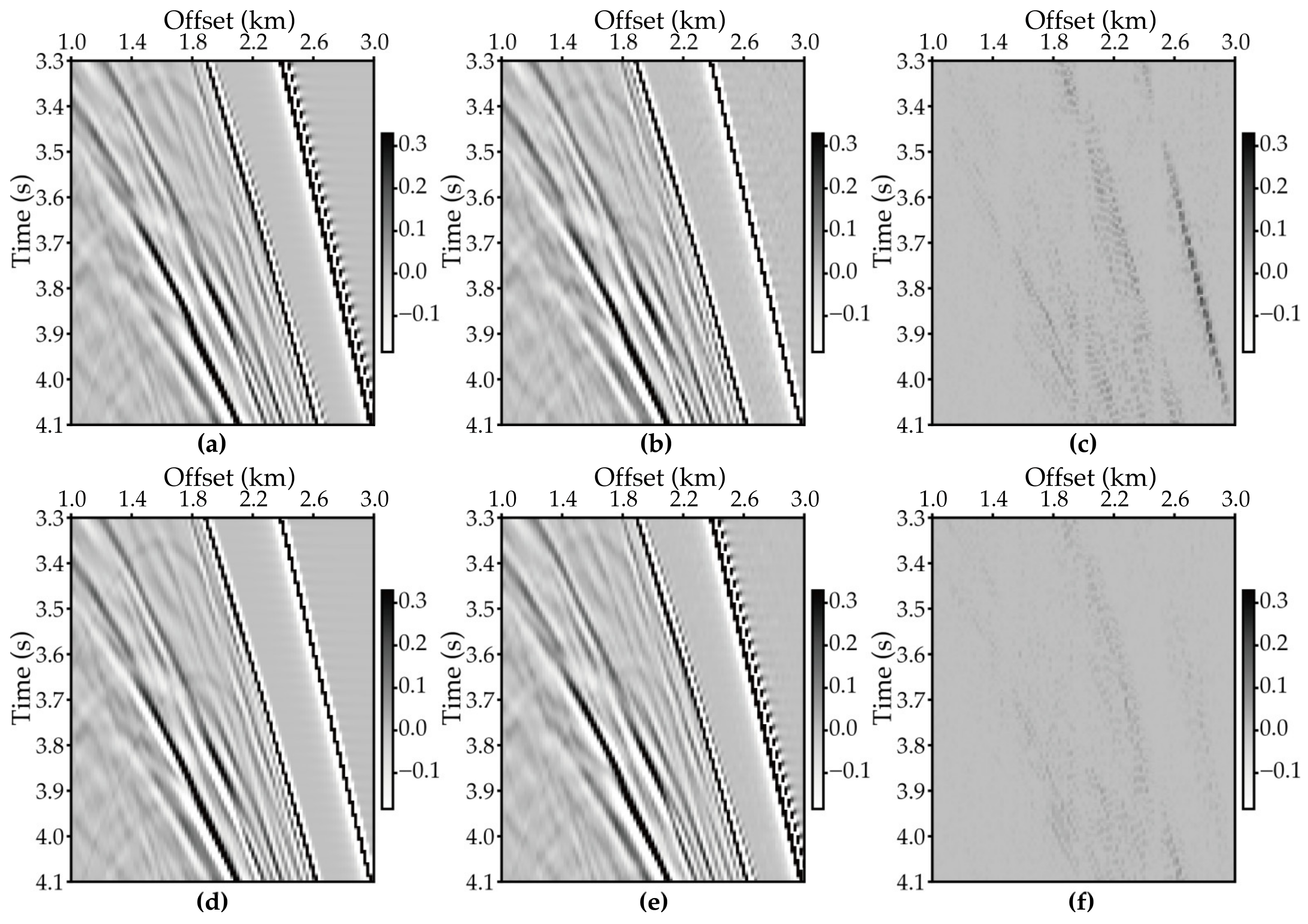
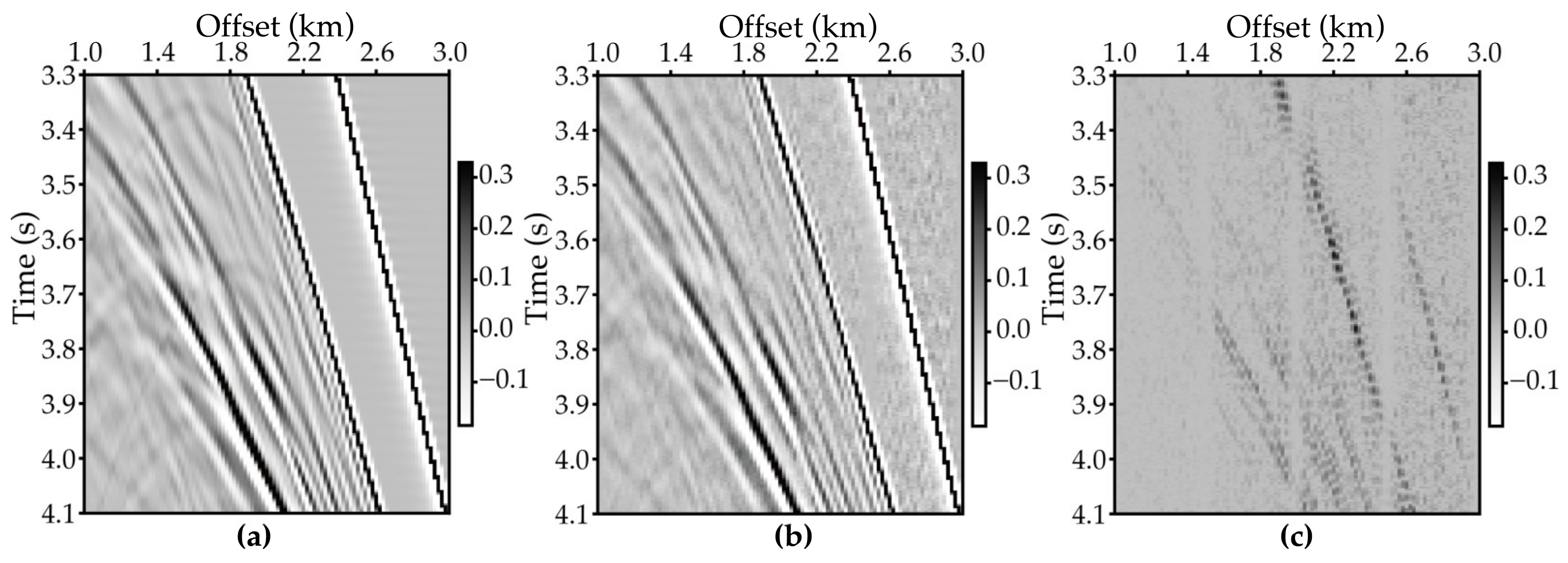
As shown in Figure 1 the workflow we proposed, the Inverse Model is trained to eliminate time dispersion of large time-step (i.e., 1.2 ms) unlabeled data set, and the Forward Model is used for regularizing the training by semi-supervised learning mapping small time-step data (i.e., 0.2 ms) to large time-step data (i.e., 1.2 ms). Figure 6 and Figure 7 show the results at the time from 3.81 s to 4.23 s of Trace No. 500 by the Inverse Model and the Forward Model, respectively. Results for the shot profiles are shown in Figure 8, and the enlarged views of the red box areas in the results are shown in Figure 9. It is evident that the dispersion artifacts in large time-step data, as seen in Figure 9a, are suppressed by the proposed Inverse Model as seen in Figure 9b, and the results are similar to the corresponding small time-step data in Figure 9d. Figure 9e shows the output of Forward Model, which has visible dispersion artifacts, are inputted by the small time-steps data as seen in Figure 9d, and the results in Figure 9e are similar to large time-steps data in Figure 9a. Figure 9c shows the difference between Figure 9b,d while Figure 9f displays the difference between Figure 9a,e.
We choose five different metrics to measure the performance of the proposed method: mean absolute error (L1 Loss), Pearson’s correlation coefficient (PCC), coefficient of determination (r2), peak signal-to-noise ratio (PSNR/dB), and structural similarity index (SSIM) between target and the prediction. PCC is a metric that measures the linear relationship between the estimated and target traces, and r2 is a goodness-of-fit metric that takes the mean squared error between the two traces; both metrics are often used to assess the overall fit of two traces. PSNR is used to compare the quality of output image and the original image, and SSIM measures the similarity between the two images. The quantitative outcomes are computed using the training and testing traces. In this, we have modified the L1 Loss (L1) to better fit our proposed workflow. Specifically, the L1 Loss is the sum of the squares of all corresponding location differences:
L = α N L 1 ( y p r e d ,   y ) + β N L 1 ( f w F ( f w I ( x u ) ) ,   x )
where N = 2001 is the number of one trace data points, L 1 represents the original L1 Loss, and the modified L1 Loss is set as L . The result is shown in Table 1.
The results in Table 1 demonstrate that the suggested workflow performs almost as well on validation data as it does on training data, demonstrating its generalizability beyond training data.

3.2. The Data Test with the SEAM Model

In this part, the data set is generated by using the compiled program with the velocity model of SEAM (Figure 10).
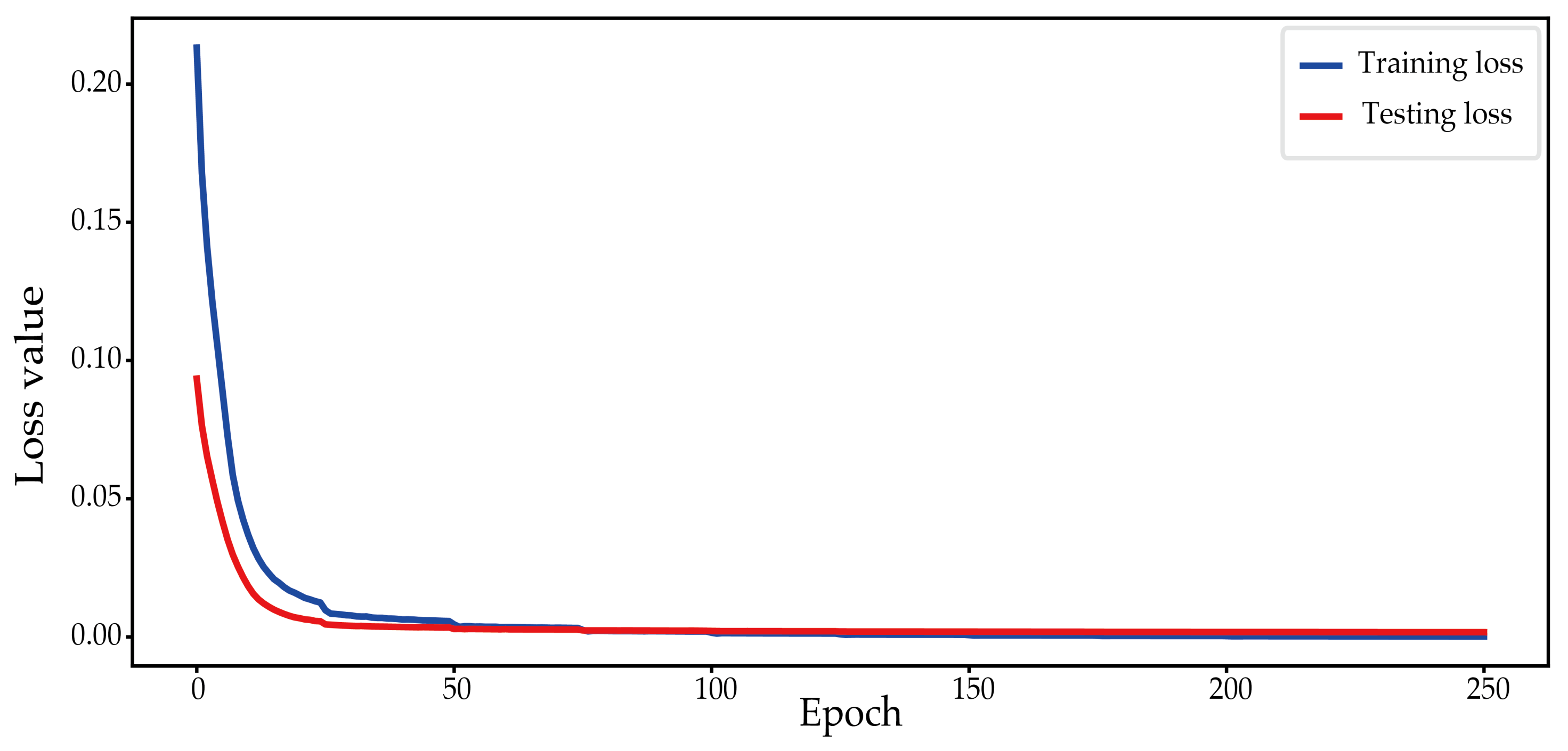
To create the data set, we choose the time step of 0.4 ms and 2 ms, assuming that the solution obtained on the 0.4 ms time step is approximated as time-dispersion-free data. The data set contains 12 shots, each of which contains a receiver spacing of 20 m between the receiver array, and each shot contains 325 traces, each trace with 2001 time sampling points by re-sampling to the time interval of 4 ms. In this training, we choose 5 shots for training and 7 shots for testing. Considering the small size of the SEAM data set, we adjust the batch size to 5, and the Inverse Model and Forward Model are together trained for 250 epochs. Next, we follow the training procedure. Figure 11 shows that the loss function curve leveled off.
Here, we adopt a new training approach—transfer learning—to evaluate the performance of the method. Considering that the Marmousi model has sufficient training data and performs well on the test data sets, we apply transfer learning with the trained Marmousi model, and we fix the initialization of the Local pattern analysis submodule by Marmousi model weights file, and then continue training the SEAM data set. The remainder of the steps are the same as the previous training process.
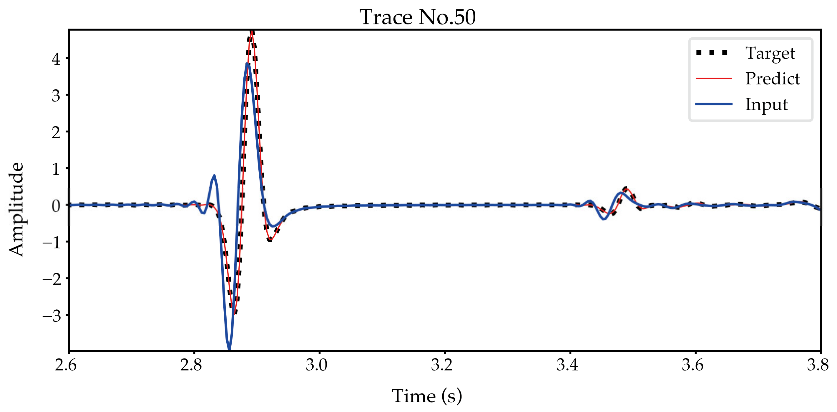
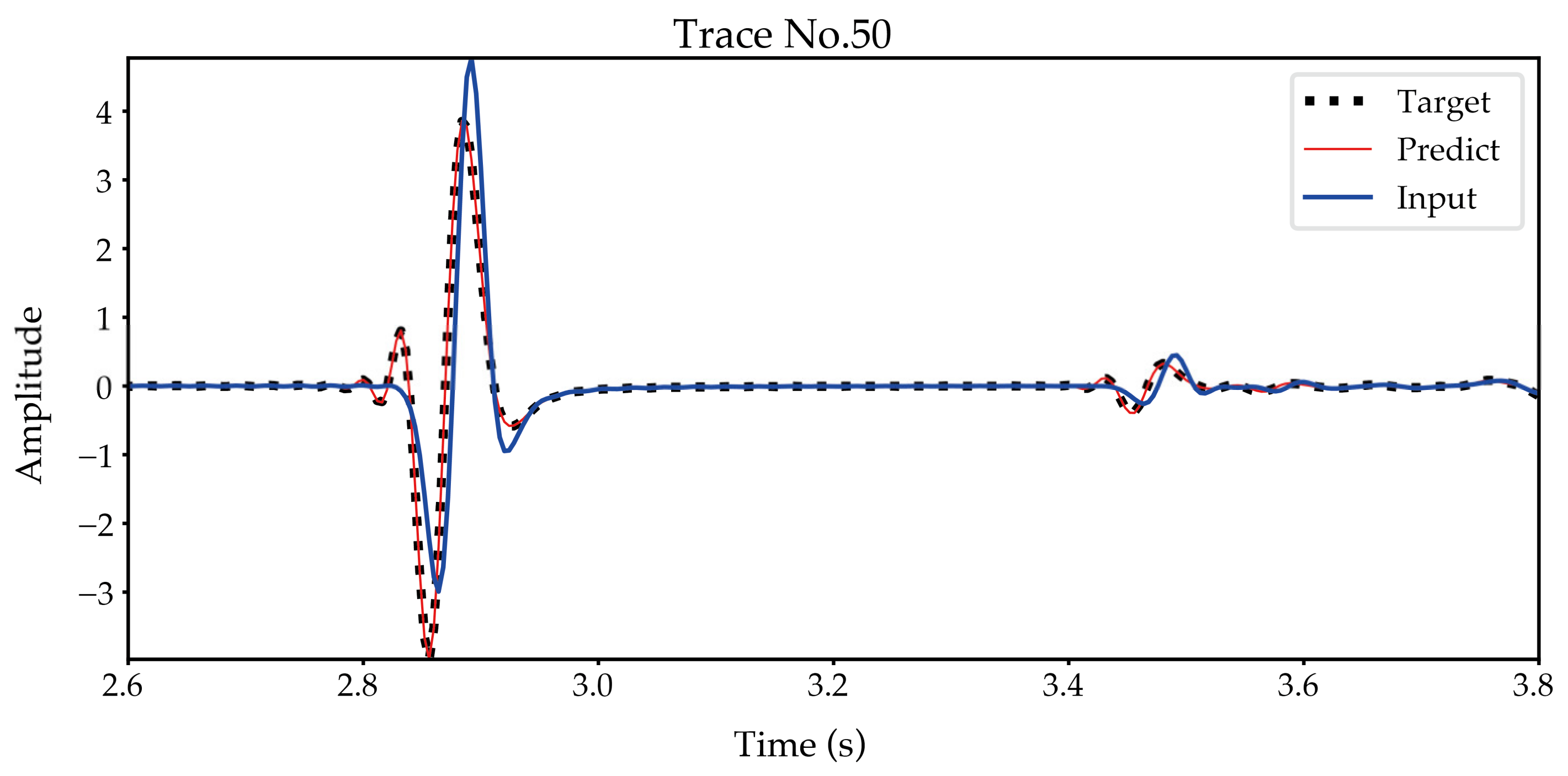
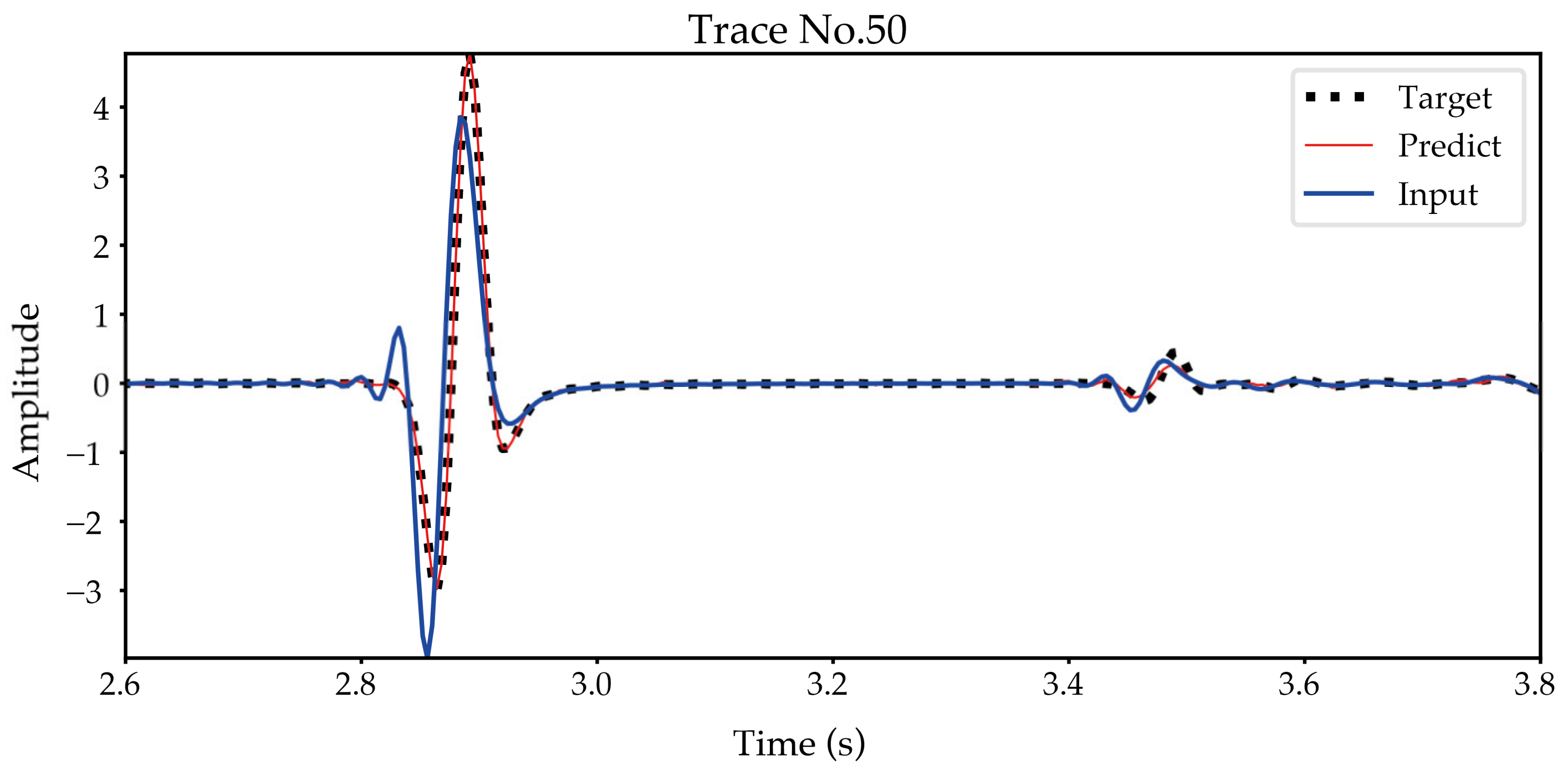
As shown in Figure 1 the workflow we proposed, the Inverse Model is trained to eliminate time dispersion of large time-step (i.e., 2 ms) unlabeled data set, and the Forward Model is used for regularizing the training by semi-supervised learning mapping small time-step data (i.e., 0.4 ms) to large time-step data (i.e., 2 ms). Figure 12 and Figure 13 show the result at the time from 2.6 s to 3.8 s of Trace No. 50 by the Inverse Model and the Forward Model, respectively. Results for the shot profiles are shown in Figure 14, and the enlarged views of the results are shown in Figure 15. It is evident that the dispersion artifacts in large time-step data, as seen in Figure 15a, are mitigated by the proposed Inverse Model as seen in Figure 15b, and the results are similar to small time-step data shown in Figure 15d. Figure 15e shows the output using Forward Model, which has visible dispersion artifacts, are inputted by the small time-step data as seen in Figure 15d, and the results in Figure 15e are similar to large time-step data in Figure 13a. Figure 13c shows the absolute difference between Figure 13b and d while Figure 13f displays the difference between Figure 13a,e.
Similar to the Marmousi model, we choose five different metrics to measure the performance of the proposed methods: Pearson’s correlation coefficient (PCC), coefficient of determination (r2), modified L1 Loss (L), peak signal-to-noise ratio (PSNR/dB), and structural similarity index (SSIM) between target and the mean prediction. The results are shown in Table 2.

4. Discussion

In this work, the given network is designed to map the data simulated by a compiled program using two designated time intervals. Hence, re-training is required whenever the modeling algorithm, time interval, or frequency band is changed. This is because, as in all deep learning methods, training a neural network on one data set and then applying it to another data set requires that both data sets have the same distribution; otherwise, the test data will be incorrect due to overfitting. Considering the computational effort associated with re-training, on the new seismic model, we propose transfer learning to overcome this problem. When we test the proposed strategy on the SEAM model using the transfer learning training approach, we regard Marmousi as a pre-training seismic model. However, the Marmousi model should have enough training data and perform well on the test data sets, otherwise, the SEAM model data set may not work well with small amounts of data.
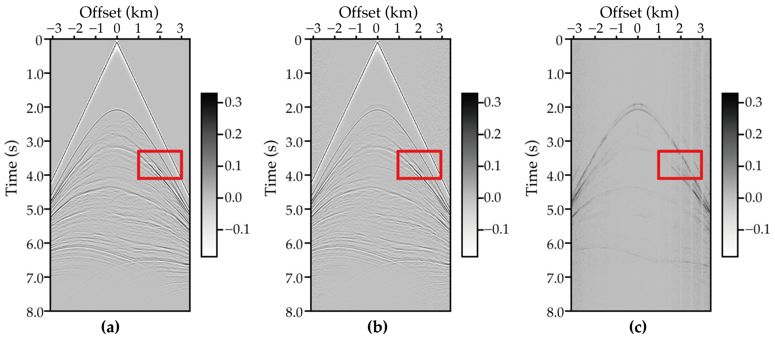
Additionally, as a comparison, we built a standard GRU network to eliminate time dispersion. This GRU network is from Pytorch machine learning library, and the size of input and output are the same as our proposed network. The data from the SEAM model are used for test. The results are shown in Figure 16, Figure 17 and Figure 18. As can be seen, the GRU deep-learning model can also eliminate the time dispersion but less effective than the proposed semi-supervised deep-learning model. This experiment demonstrates that many deep-learning models can achieve time-dispersion elimination but the performance may be different.

5. Conclusions

Seismic wavefield simulation is a key component of seismic data imaging and inversion. Finite-difference (FD) methods are the most widely used technique, but it suffers from time and spatial dispersion. In the case where only a pre-compiled software is available, the FD scheme/algorithm is unknown, and it becomes a black box to user. Therefore, it is hard to predict the time dispersion mathematically. Herein, we propose using deep learning methods to overcome this problem.
In this study, we use CNNs and GRUs with semi-supervised learning to eliminate time dispersion of seismic records. We estimate the proposed Inverse Model and Forward Model by training the network with a few shots generated by a compiled modeling program. The training data sets include labeled and unlabeled data sets. The labeled data set is a paired data set with large time-step data (with time dispersion) and their corresponding small time-steps data (without time dispersion). The unlabeled data set is the large time-step data that need time-dispersion elimination. We then apply this network to the unlabeled data sets. In addition, re-training is required whenever the modeling algorithm, time interval, or frequency band is changed, so we propose a transfer learning training method to extend from the trained model to another model, which reduces the computational load caused by re-training. Numerical tests on different models indicate that the proposed method is capable of sufficiently eliminating the time dispersion. The networks and examples presented in the paper can be accessed via https://github.com/wavetomo/Timedispersion (accessed on 10 October 2020).

Author Contributions

Conceptualization, G.Y. and D.W.; Data curation, B.W.; Formal analysis, Y.H.; Investigation, X.M.; Methodology, Y.H.; Supervision, D.W.; Validation, Y.H.; Writing—original draft, Y.H.; Writing—review & editing, Y.H. All authors have read and agreed to the published version of the manuscript.

Funding

This work is supported by National Key R&D Program of China (No. 2018YFA0702502), R&D Department of China National Petroleum Corporation (Investigations on fundamental experiments and advanced theoretical methods in geophysical prospecting applications, 2022DQ0604 -02), NSFC (Grant No. 41974142, 42074129), Science Foundation of China University of Petroleum (Beijing) (Grant No. 2462020YXZZ005), and State Key Laboratory of Petroleum Resources and Prospecting (Grant No. PRP/indep-4- 2012).

Conflicts of Interest

The authors declare no conflict of interest.

References

  1. Li, Z.-C.; Qu, Y.-M. Research progress on seismic imaging technology. Pet. Sci. 2022, 19, 128–146. [Google Scholar] [CrossRef]
  2. Baysal, E.; Dan, D.K.; Sherwood, J. Reverse-Time Migration. Geophysics 1983, 48, 1514–1524. [Google Scholar] [CrossRef] [Green Version]
  3. Wu, B.; Yao, G.; Cao, J.-J.; Wu, D.; Li, X.; Liu, N.-C. Huber inversion-based reverse-time migration with de-primary imaging condition and curvelet-domain sparse constraint. Pet. Sci. 2022, 19, 1542–1554. [Google Scholar] [CrossRef]
  4. Tarantola, A. Inversion of seismic reflection data in the acoustic approximation. Geophysics 1984, 49, 1259–1266. [Google Scholar] [CrossRef]
  5. Yao, G.; Wu, D. Reflection full waveform inversion. Sci. China Earth Sci. 2017, 60, 1783–1794. [Google Scholar] [CrossRef] [Green Version]
  6. Wang, Z.-Y.; Huang, J.-P.; Liu, D.-J.; Li, Z.-C.; Yong, P.; Yang, Z.-J. 3D variable-grid full-waveform inversion on GPU. Pet. Sci. 2019, 16, 1001–1014. [Google Scholar] [CrossRef] [Green Version]
  7. Etgen, J.T. High Order Finite-Difference Reverse Time Migration with the Two Way Nonreflecting Wave Equation; Stanford University: Stanford, CA, USA, 1986; pp. 133–146. [Google Scholar]
  8. Yang, L.; Sen, M.K. A new time–space domain high-order finite-difference method for the acoustic wave equation. J. Comput. Phys. 2009, 228, 8779–8806. [Google Scholar]
  9. Yao, G.; da Silva, N.V.; Debens, H.A.; Wu, D. Accurate seabed modeling using finite difference methods. Comput. Geosci. 2018, 22, 469–484. [Google Scholar] [CrossRef] [Green Version]
  10. Song, X.; Fomel, S.; Ying, L. Lowrank finite-differences and lowrank Fourier finite-differences for seismic wave extrapolation in the acoustic approximation. Geophys. J. Int. 2013, 193, 960–969. [Google Scholar] [CrossRef]
  11. Sun, J.; Fomel, S.; Ying, L. Low-rank one-step wave extrapolation for reverse time migration. Geophysics 2016, 81, S39–S54. [Google Scholar] [CrossRef]
  12. Zhang, J.-H.; Yao, Z.-X. Optimized finite-difference operator for broadband seismic wave modeling. Geophysics 2013, 78, A13–A18. [Google Scholar] [CrossRef]
  13. Liu, Y. Research progress on time-space domain finite-difference numerical solution and absorption boundary conditions of wave equation. Oil Geophys. Prospect. 2014, 49, 35–46. [Google Scholar]
  14. Yang, L.; Yan, H.; Liu, H. Optimal staggered-grid finite-difference schemes based on the minimax approximation method with the Remez algorithm. Geophysics 2017, 82, T27–T42. [Google Scholar] [CrossRef]
  15. Kosloff, D.; Pestana, R.C.; Tal-Ezer, H. Acoustic and elastic numerical wave simulations by recursive spatial derivative operators. Geophysics 2010, 75, T167–T174. [Google Scholar] [CrossRef]
  16. Yang, L. Optimal staggered-grid finite-difference schemes based on least-squares for wave equation modelling. Geophys. J. Int. 2014, 197, 1033–1047. [Google Scholar]
  17. Ren, Z.; Liu, Y. Acoustic and elastic modeling by optimal time-space-domain staggered-grid finite-difference. Geophysics 2015, 80, T17–T40. [Google Scholar] [CrossRef]
  18. Wang, E.; Liu, Y.; Sen, M.K. Effective finite-difference modelling methods with 2-D acoustic wave equation using a combination of cross and rhombus stencils. Geophys. J. Int. 2016, 206, 1933–1958. [Google Scholar] [CrossRef]
  19. Kosloff, D.D.; Baysal, E. Forward modeling by a Fourier method. Geophysics 1982, 47, 1402–1412. [Google Scholar] [CrossRef] [Green Version]
  20. Fornberg, B. The pseudospectral method; comparisons with finite differences for the elastic wave equation. Geophysics 1987, 52, 483–501. [Google Scholar] [CrossRef]
  21. Dablain, M. The application of high-order differencing to the scalar wave equation. Geophysics 1986, 51, 54–66. [Google Scholar] [CrossRef]
  22. Blanch, J.O.; Robertsson, J. A modified Lax-Wendroff correction for wave propagation in media described by Zener elements. Geophys. J. Int. 1997, 131, 381–386. [Google Scholar] [CrossRef] [Green Version]
  23. Soubaras, R.; Yu, Z. Two-step Explicit Marching Method for Reverse Time Migration. In SEG Technical Program Expanded Abstracts 2008; Society of Exploration Geophysicists: Huston, TX, USA, 2008. [Google Scholar]
  24. Amundsen, L.; Pedersen, Ø. Time step n-tupling for wave equations. Geophysics 2017, 82, T249–T254. [Google Scholar] [CrossRef]
  25. Liu, Y.; Sen, M.K. Time–space domain dispersion-relation-based finite-difference method with arbitrary even-order accuracy for the 2D acoustic wave equation. J. Comput. Phys. 2013, 232, 327–345. [Google Scholar] [CrossRef]
  26. Tan, S.; Huang, L. An efficient finite-difference method with high-order accuracy in both time and space domains for modelling scalar-wave propagation. Geophys. J. Int. 2014, 197, 1250–1267. [Google Scholar] [CrossRef]
  27. Ren, Z.; Li, Z.; Liu, Y.; Sen, M.K. Modeling of the Acoustic Wave Equation by Staggered-Grid Finite-Difference Schemes with High-Order Temporal and Spatial AccuracyTemporal High-Order Finite Difference. Bull. Seismol. Soc. Am. 2017, 107, 2160–2182. [Google Scholar] [CrossRef]
  28. Ren, Z.-M.; Dai, X.; Bao, Q.-Z. Source wavefield reconstruction based on an implicit staggered-grid finite-difference operator for seismic imaging. Pet. Sci. 2022. [Google Scholar] [CrossRef]
  29. Stork, C. Eliminating Nearly All Dispersion Error from FD Modeling and RTM with Minimal Cost Increase. In Proceedings of the 75th Eage Conference en Exhibition Incorporating SPE Europec, London, UK, 10–13 June 2013. [Google Scholar]
  30. Wang, M.; Xu, S. Finite-difference time dispersion transforms for wave propagation. Geophysics 2015, 80, WD19–WD25. [Google Scholar] [CrossRef]
  31. Li, Y.E.; Wong, M.; Clapp, R. Equivalent accuracy at a fraction of the cost: Overcoming temporal dispersion. Geophysics 2016, 81, T189–T196. [Google Scholar] [CrossRef] [Green Version]
  32. Koene, E.; Robertsson, J.; Broggini, F.; Andersson, F. Eliminating time dispersion from seismic wave modeling. Geophys. J. Int. 2018, 213, 169–180. [Google Scholar] [CrossRef]
  33. Wang, Y.-Q.; Wang, Q.; Lu, W.-K.; Ge, Q.; Yan, X.-F. Seismic impedance inversion based on cycle-consistent generative adversarial network. Pet. Sci. 2022, 19, 147–161. [Google Scholar] [CrossRef]
  34. Yuan, S.; Jiao, X.; Luo, Y.; Sang, W.; Wang, S. Double-scale supervised inversion with a data-driven forward model for low-frequency impedance recovery. Geophysics 2022, 87, R165–R181. [Google Scholar] [CrossRef]
  35. Gadylshin, K.; Vishnevsky, D.; Gadylshina, K.; Lisitsa, V. Numerical dispersion mitigation neural network for seismic modeling. Geophysics 2022, 87, T237–T249. [Google Scholar] [CrossRef]
  36. Yuan, S.; Wang, J.; Liu, T.; Xie, T.; Wang, S. 6D phase-difference attributes for wide-azimuth seismic data interpretation. Geophysics 2020, 85, IM37–IM49. [Google Scholar] [CrossRef]
  37. Alfarraj, M.; AlRegib, G. Semi-supervised learning for acoustic impedance inversion. In SEG Technical Program Expanded Abstracts 2019; Society of Exploration Geophysicists: Huston, TX, USA, 2019; pp. 2298–2302. [Google Scholar]
  38. Cho, K.; van Merriënboer, B.; Bahdanau, D.; Bengio, Y. On the properties of neural machine translation: Encoder–decoder approaches. In Proceedings of the 8th Workshop on Syntax, Semantics and Structure in Statistical Translation, SSST 2014, Doha, Qatar, 25 October 2014; pp. 103–111. [Google Scholar]
  39. Yu, F.; Koltun, V. Multi-Scale Context Aggregation by Dilated Convolutions. In Proceedings of the 4th International Conference on Learning Representations, ICLR 2016, San Juan, Puerto Rico, 2–4 May 2016. [Google Scholar]
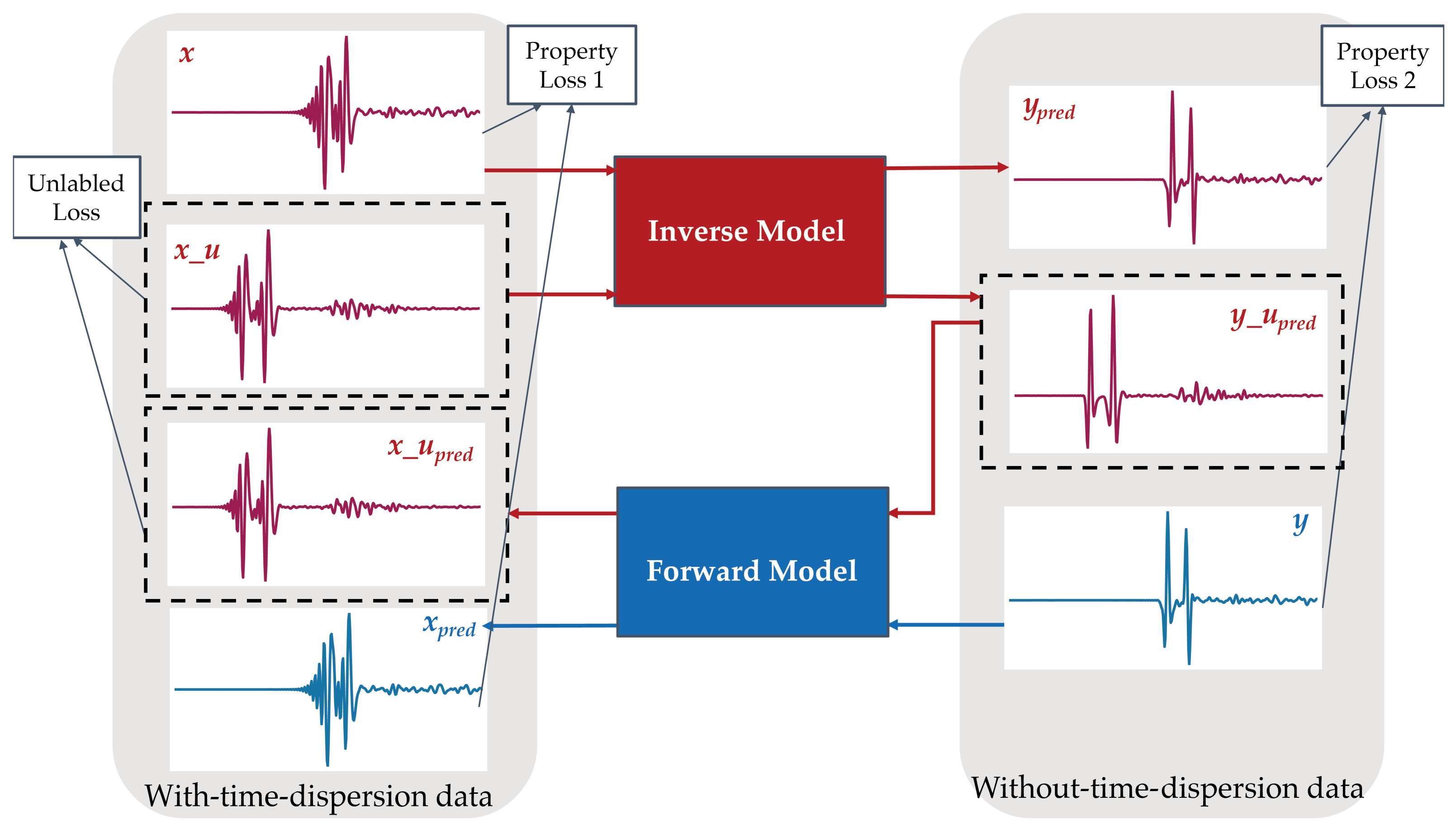
Figure 1. The proposed workflow. Here, x is the labeled single trace of time-dispersed data, its corresponding target time-dispersion-free data is labeled as y , and x _ u is the unlabeled single trace of time-dispersed data. x is mapped to y p r e d by the Inverse Model, and then y p r e d with y calculates property loss 1; unlabeled data (in the dashed black box) x_u is mapped to y _ u p r e d by the Inverse Model, then y _ u p r e d is mapped to x _ u p r e d by the Forward Model, and x _ u p r e d with x _ u calculate the unlabeled loss. y is mapped to x p r e d by the Forward Model, and then x p r e d with x calculate property loss 2. Specifically, property loss 1 adds property loss 2 as property loss; both property loss and unlabeled loss are used for updating the weights of the Inverse Model and Forward Model.
Energies 15 07701 g001
Figure 2. The architecture of the Inverse Model in the proposed workflow. Sequence Modeling submodule includes GRU, whose input traces are modeled as sequential data, and temporal features are computed based on these temporal variations. Local Pattern Analysis submodule includes three parallel 1D CNN modules, with each parallel 1D CNN module (ConvBlock) having the same convolutional kernel size but different dilation coefficients. The outputs of each parallel 1D CNN module (ConvBlock) are stitched together and fed into a 1D CNN module (ConvBlock) with three layers and decreasing convolutional kernels (kernel = k). Regression is used for mapping the extracted features from the other submodules to the target data.
Energies 15 07701 g002
Figure 3. The architecture of the Forward Model in the proposed workflow. This is similar to the Inverse Model, the differences are 2 times the GRU output data size and two fully connected-layer modules in the Sequence Modeling submodule.
Energies 15 07701 g003
Figure 4. The velocity model of a partial modified Marmousi.
Energies 15 07701 g004
Figure 5. The loss function curve during the prediction for the Marmousi model. The training error and testing error decrease fast and then converge to a small value.
Energies 15 07701 g005
Figure 6. The comparison at the time from 3.81 to 4.23 s between the predicted trace and the input trace of the Inverse Model. The black dotted line indicates the target trace without time dispersion (0.2 ms time step). The blue and red lines represent the input with time dispersion (1.2 ms time step) and output data after the time dispersion elimination, respectively.
Energies 15 07701 g006
Figure 7. The comparison at the time from 3.81 s to 4.23 s between the predicted trace and the input trace of the Forward Model. The black dotted line indicates the target trace with time dispersion (1.2 ms time step). The blue and red lines represent the input without time dispersion (0.2 ms time step) and predicted data with time dispersion, respectively.
Energies 15 07701 g007
Figure 8. The profiles of seismic forward modeling records. (a) The forward modeling result with a time step of 1.2 ms. (b) The result after time dispersion elimination using the network. (a,b) are the input and output of Inverse Model, respectively. (c) The absolute difference from (b,d). (d) The forward modeling result with a time step of 0.2 ms, which is the input of the Forward Model. (e) The output of Forward Model, which contains time dispersion. (f) The absolute difference from (a,e).
Energies 15 07701 g008
Figure 9. Enlarged view of the red box areas in (af) of Figure 8. The order of the plots is the same as that of Figure 8.
Energies 15 07701 g009
Figure 10. The velocity model of a part of SEAM.
Energies 15 07701 g010
Figure 11. The loss function curve during the training of the SEAM model. The training error and testing error decrease fast and then converge to a small value.
Energies 15 07701 g011
Figure 12. The comparison at the time from 2.6 s to 3.8 s between the predicted trace and the input trace by the Inverse Model. The black dotted line indicates the target trace without time dispersion (0.4 ms time step). The blue and red lines represent the input (2 ms time step) and predicted data after time-dispersion elimination, respectively.
Energies 15 07701 g012
Figure 13. The comparison at the time from 2.6 s to 3.8 s between the predicted trace and the input trace by the Forward Model. The black dotted line indicates the target trace with time dispersion (2 ms time step). The blue and red lines represent the input (0.4 ms time step) and predicted data with time dispersion, respectively.
Energies 15 07701 g013
Figure 14. The profiles of seismic forward modeling records. (a) The forward modeling result with a time step of 2 ms. (b) The result after time dispersion elimination using the network. (a,b) are the input and output of Inverse Model, respectively. (c) The absolute difference from (b,d). (d) The forward modeling result with a time step of 0.4 ms, which is the input of the Forward Model. (e) The output of Forward Model, which contains time dispersion. (f) The absolute difference from (a,e).
Energies 15 07701 g014
Figure 15. Enlarged view of the red box areas in (af) of Figure 14. The order of the plots is the same as that of Figure 14.
Energies 15 07701 g015
Figure 16. The comparison at the time from 2.6 s to 3.8 s between the predicted trace and the input trace for the GRU Model. The black dotted line indicates the target trace without time dispersion (0.4 ms time step). The blue and red lines represent the input (2 ms time step) and predicted data after time-dispersion elimination, respectively.
Energies 15 07701 g016
Figure 17. The profiles of seismic forward modeling records. (a) The forward modeling result with a time step of 0.4 ms. (b) The result after time dispersion elimination using the GRU Model. (c) The absolute difference between (a) and (b).
Energies 15 07701 g017
Figure 18. Enlarged view of the red box areas in (ac) of Figure 17. The order of the plots is the same as that of Figure 17.
Energies 15 07701 g018
Table 1. Performance metrics of the trained network on the Marmousi model.
MetricTrainingValidation
PCC0.99990.9997
r20.99990.9995
L7.19 × 10−52.67 × 10⁻⁴
PSNR91.220586.7756
SSIM1.00001.0000
Table 2. Performance metrics of the trained network on the SEAM model.
MetricTrainingValidation
PCC1.00000.9993
r21.00000.9984
L1.70 × 10−58.09 × 10⁻⁴
PSRN94.650179.9299
SSIM1.00001.0000
Publisher’s Note: MDPI stays neutral with regard to jurisdictional claims in published maps and institutional affiliations.