Abstract
Aiming at the problem of unbalanced data categories of UHV converter valve fault data, a method for UHV converter valve fault detection based on optimization cost-sensitive extreme random forest is proposed. The misclassification cost gain is integrated into the extreme random forest decision tree as a splitting index, and the inertia weight and learning factor are improved to construct an improved particle swarm optimization algorithm. First, feature extraction and data cleaning are carried out to solve the problems of local data loss, large computational load, and low real-time performance of the model. Then, the classifier training based on the optimization cost-sensitive extreme random forest is used to construct a fault detection model, and the improved particle swarm optimization algorithm is used to output the optimal model parameters, achieving fast response of the model and high classification accuracy, good robustness, and generalization under unbalanced data. Finally, in order to verify its effectiveness, this model is compared with the existing optimization algorithms. The running speed is faster and the fault detection performance is higher, which can meet the actual needs.
1. Introduction
The DC transmission system can run continuously for a long time [1], and the converter valve, as a powerful and stable core piece of equipment in the DC transmission system, plays a very crucial role. Only correct state assessment and fault detection of the core equipment in the system can reduce the failure rate to a minimum and make the power grid operate at a stable and safe level [2]. In the DC transmission systems currently under construction in the world, the increasing scale has placed higher demands on the reliability of power system fault detection [3,4].
In the early fault detection of the converter valve, the operation and maintenance personnel observe the equipment with the naked eye and then roughly judge the fault type, to determine which maintenance method to adopt. Using the naked eye to observe is prone to omissions and inaccurate judgments and is easily affected by weather. After that, the 39 state parameters of the three components are mainly provided by the “Guidelines for State Evaluation of HVDC Converter Valves” [5] (hereinafter referred to as “Guidelines”), and the state of each state parameter is first judged. Then, the form of scoring is taken and the total score is calculated to finally judge the operating status of the converter valve to take countermeasures. As this method uses a scoring method that requires manual scoring, it will result in lower evaluation efficiency and may not be able to complete the evaluation task in time. In addition, although the 39 state parameters provided by the “Guidelines” provide a comprehensive evaluation of the overall operating state of the converter valve, there are parameters that have little effect on the overall evaluation, and some of the parameters have too strong a commonality. When the flow valve is used for data collection, collecting these data will only increase the ineffective workload [6]. Under the influence of the precise structure and complex fault types of the converter valve, the complete fault detection system based on the converter valve is not mature enough.
With the continuous advancement of science and technology, various detection methods have emerged one after another, and the evaluation and detection methods have gradually transformed into intelligent, precise, stable, and high-efficiency methods, bringing new research ideas and technical strategies to the research on converter valve fault detection in order to obtain higher work efficiency, safer electricity consumption, and accelerated optimization of industrial upgrading, providing a strong guarantee. Fault detection methods can be divided into model-based methods [7], data-based methods [8], and signal-processing-based methods [9]. Reference [10] adopted an efficient machine learning method combining random forest (RF) and extreme gradient boosting (XGBoost). The proposed model has good robustness and has certain advantages over support vector machines in processing multi-dimensional data. In Reference [11], random forest (RF) and AdaBoost models were investigated for islanding detection techniques for synchronous power generation, the performance was quantified using parameters such as total harmonic distortion (THD), and the experiments showed that the proposed model has high accuracy and good robustness. In Reference [12], a typical correlation analysis (CCA) based on real-time-learning (JITL)-assisted monitoring and fault detection of multimode processes was proposed. To reduce the time to search for relevant data, K-means was integrated into JITL to construct a local CCA model, and the superiority of the proposed scheme was verified using an industrial benchmarking approach. Reference [13] combined the correlation statistical analysis with sliding windows and validated the effectiveness of the proposed method in thermal power plant processes using a recursive algorithm with low computational complexity based on the increased computational cost, and controlled the width of the sliding window by a stochastic algorithm. The above methods have limitations in terms of fault detection range, detection accuracy, and learning speed, and extreme random forest based on cost sensitivity has better performance in dealing with numerous complex data samples or unbalanced data, which is more suitable for the current needs of transducer valve fault detection.
In the context of increasingly common intelligent algorithms, the imbalance of data samples for converter valves is still a major challenge. Due to the high reliability of the commutation valves currently put into operation in China, there are much more normal operation data samples of the commutation valves than those of the nonnormal operation, resulting in an imbalance in data samples. Cost sensitivity is a relatively novel method in the field of machine learning, which assigns different costs to different types of errors, so the sum of the costs of misclassification is minimized when classifying, and a high accuracy of classification is achieved. Numerous scholars have conducted extensive research for this method. Reference [14] proposed a cost-sensitive deep neural network, and the proposed model does not change the original distribution of the data during the training process, reduces the computational cost, and has a more robust and superior performance compared with the existing mainstream sampling techniques. Reference [15] proposed a cost-sensitive multiset feature learning to construct multiple balanced subsets by random partitioning to construct a depth-metric-based UCML (DM-UCML) method with greater robustness when using highly unbalanced datasets. Reference [16] proposed a date-driven incremental interpolation model (DIM) that can efficiently fill in missing values for all available information in the dataset, and proposed a new scoring criterion by considering economic criteria and valid interpolation information to rank the missing features. The proposed method was validated on the UCI dataset with some improvement in accuracy. When the cost-sensitive strategy is used to optimize the classifier performance, there is still the problem that it is difficult to use the model hyperparameters to tune the parameters, which still has some impact on the overall performance of the model. Based on this, an optimization algorithm was used for optimal parameter selection to further improve the model performance [17]. The improved particle swarm optimization algorithm [18] was constructed by designing adaptive learning factors and inertia factors to find the optimal parameters of the cost-sensitive extreme random forest model and improve the model accuracy.
Through the above analysis, the UHV converter valve fault detection based on the optimization cost-sensitive extreme random forest (CS-ERF) is proposed for the complex fault types of the converter valve. First, the converter valve is introduced by 39 converter valve state quantities, and the initial state assessment of the converter valve is performed. Then, data cleaning and feature selection are performed on the source data to reduce the feature dimension of the data and remove the redundant features. Then, the sample dataset is divided into two categories, the training set and test set, and the training set is used to train the model and the test set is used to test and evaluate the model prediction accuracy. Finally, based on the optimization cost-sensitive extreme random forest algorithm, the parameter values of the optimal model are found using an improved particle swarm optimization algorithm, and the splitting indicator of the cost-sensitive decision tree is chosen as the misclassification cost gain. The results improve the classification accuracy and overall performance of the model while reducing the impact of unbalanced samples on branch nodes, and also avoid the problems of model bias toward the majority class caused by large normal sample data and very few fault data samples, and low accuracy in identifying data samples for fault states, with higher real-time performance, lower false alarm rate, and higher gMean value.
2. Particle Swarm Optimization Algorithm
Particle Swarm Optimization (PSO) originated in 1995 [19], inspired by the regularity of bird flock foraging, based on the research on flock foraging behavior; that is, through collective information sharing, the group can find the most optimal solution. The algorithm has the advantages of simplicity, easy implementation, fast convergence, and few parameters. For high-dimensional data processing problems, it converges to the optimal solution faster than the genetic algorithm does.
2.1. Basic Theory of PSO Algorithm
The process of a flock of birds going out to find food is very similar to the process of humans planning things together. When a flock of birds goes out to look for food, initially, all the birds do not know exactly which location or direction has the most food and each bird searches for food randomly, and as the number of times and the time increases, they gradually learn to share information and continue the next search based on the search experience of the other birds. Gradually, they form a flock, searching for the same goal.
Each particle in the PSO algorithm has an adaptation value, which is determined by the function being optimized. The two basic properties of the particles are velocity and position, which are also the two core elements of the PSO algorithm, and the direction and distance of the particles are determined by the velocity [19]. First, the PSO algorithm randomly initializes a group of particles and then finds the optimal solution by updating iterations. The optimal solution is divided into the local optimal solution and global optimal solution, and each particle can determine the location of the current best region based on the existing experience and information, which is the local optimal solution. Meanwhile the location of the best region obtained from the experience information of all particles is the global optimal solution. In each update iteration, each particle updates the velocity and position of the particle by comparing these two optimal solutions [20].
2.2. PSO Algorithm Formula Implementation
Suppose the target search space is a D-dimensional space, and the particle population has M particles, in which the position of the t-th particle can be represented by a D-dimensional vector as:
The velocity of the t-th particle is:
The local optimal solution searched by the t-th particle:
The global optimal solution searched by the entire particle swarm:
The fitness value of the optimal area searched by the t-th particle (also the value of the optimization objective function) is (the optimal fitness value in the search history of a single particle), and the fitness value of the optimal area searched by the particle swarm is (the particle swarm searches for the best fitness value in the history).
On the basis of obtaining the local optimal solution and the global optimal solution, in order to obtain the final result at the fastest speed [21], each particle can update its speed and position according to the following formulas:
- 1.
- Speed update formula:
- 2.
- Position update formula:
The velocity direction of each particle iteration is a vector sum of the inertial direction, the local optimum direction, and the global optimum direction, as shown in Figure 1.

Figure 1.
Schematic diagram of speed direction update.
2.3. Improved PSO Algorithm
Because the particle swarm algorithm has a fast convergence speed, the selection of parameters is very important. The setting of the number of particles, inertia factor, and constant largely determines the optimization performance of the PSO algorithm.
When the size of the particle swarm is larger, it means that the number of particles is larger, the search area for each iteration is larger, and the iterative calculation will be more complicated. The particles are initialized with an ideal local optimal solution. If the number of particles is large, the optimal solution may be found with very few iterations. Based on the above principles, the number of particles is generally selected to 25–40.
The learning factor acts on the proportion of individual experience and global experience in the allocation update iteration. When = 0, it is considered that there is no individual experience in the search process, and it is updated and iterated solely by the sharing of global social experience. The convergence speed is relatively fast, but it is easy to fall into the local optimum. When = 0, it is considered that when the particle is updating the velocity position, it only relies on individual experience and does not obtain global experience, and it is difficult to find the optimal solution at this time. In the usual case, there is = . If the former is larger, the individual tends to roam too much in its own optimal position; if the latter is larger, the particles are easily attracted to the current global optimal solution. This paper uses Equations (7) and (8) to improve the learning factor and adjust the size of and reasonably:
where are the initial value and final value of , respectively; and are the initial value and final value of , respectively; t is the corresponding iteration number; is the maximum iteration number.
The inertia factor has a great influence on the overall performance of the PSO algorithm and plays a significant role in updating the particle velocity and position. When the inertia factor is large, the particle velocity and position update will be more dependent on the particle’s own experience and history of the search, and the local search ability decreases, but the overall search ability is improved. When the inertia factor is small, the local search ability increases and the overall search ability decreases. Based on the interplay with other parameters, the inertia factor is adjusted appropriately to make the whole iterative process more inclined to the overall search, so it can complete convergence faster and improve the overall performance. In this paper, the inertia weights are adjusted and improved using a nonlinear function, as shown in Equation (9).
where and are the maximum and minimum values of ω, respectively.
In the implementation of the improved PSO (IPSO) algorithm, it mainly relies on the following procedures:
- Set the inertia factor, acceleration parameters, number of particles, and other parameters;
- Randomly initialize the velocity and position of each particle to obtain the optimal position and optimal adaptation value of the individual and the population;
- Perform n update iterations to update the velocity and position of each particle;
- Calculate and update the optimal position and optimal adaptation value of each particle, obtain the optimal position and optimal adaptation value of the population, and update the current parameters as necessary;
- Output the global optimal solution and the corresponding position variables.
3. Extreme Random Forests Based on Cost Sensitivity
3.1. Extreme Random Forest
Extremely random forest (ERF) is a derivative algorithm [10] obtained by further optimization on the basis of random forest, which is characterized by a high degree of randomness. The main difference between ERF and random forest (RF) models is that ERF does not use bagging to train each randomly selected base classifier; each of its trees is trained using the original complete training samples [22]. This approach minimizes bias. When the nodes of the decision tree are split, the general integration method obtains the optimal splitting feature and splitting threshold of the split data by calculating the evaluation criteria such as the Gini coefficient and entropy. However, when ERF calculates the score metric of each feature, it randomly selects eigenvalues. In the extreme decision tree splitting process, a feature k is selected in the sample dataset, and a value is randomly selected between the maximum and minimum value of feature k as the splitting threshold of this feature k. m split thresholds can be obtained by iterating over each feature on the dataset. The score metric of each feature is calculated, and the feature k and the threshold with the highest independent score are selected as the splitting feature and splitting threshold of the leaf node [23].
The final result of each decision tree is generated in parallel. Because the process of node splitting is relatively simple, the extreme random forest algorithm is superior to other algorithms in terms of space complexity, and the final result is determined by the voting of all decision trees. An extreme random forest is defined as follows:
where is the conditional probability, which represents the probability that the sample belongs to c in the case of vector ; D represents the tree of the decision tree. Equation (10) is the classification probability of the decision tree and Equation (11) is the principle of the final decision tree voting mechanism, using the above method for extreme random forest decision tree generation.
For the process of selected features selected as splitting features, using Equation (12) by means of a score metric, when the leaf node is split, the splitting feature is selected as the feature with the highest score, the samples smaller than the splitting threshold are put into the left leaf node after splitting, and the samples greater than or equal to the threshold are put into the right leaf node. The above steps are repeatedly recursed until the sample confusion level in the leaf node is 0 and the stop splitting condition is satisfied.
where denotes the score metric obtained by the features after calculation, and denotes the mutual information of two subsets of the node after splitting about the sample category based on the corresponding features and splitting threshold. denotes the splitting entropy of feature k. denotes the information entropy of the corresponding sample category.
3.2. Principle of Extreme Random Forest Algorithm Structure Based on Cost Sensitivity
The cost-sensitive extreme-random-forest-based algorithm is proposed for the problem of very small transducer valve fault data samples and large normal data samples, i.e., unbalanced data sample classes. First, the method introduces the misclassification cost in the evaluation criteria and changes the purpose of the fault detection decision tree from minimizing the node sample confusion and maximizing the detection accuracy to minimizing the misclassification cost. Secondly, the splitting metric is changed from the splitting feature with the highest score metric obtained by traversing all features to the misclassification cost, while the objective function of CS-ERF is set to minimize the misclassification cost. Finally, CS-ERF-based model detection results are established by a voting mechanism.
CS-ERF is a combination of cost-sensitive and extreme random forest, a derivative algorithm of ERF, and the introduction of cost sensitivity solves the problem of low detection accuracy caused by very few fault samples. The misclassification cost introduced above can be expressed here in the form of a matrix. Suppose the sample dataset contains n categories, and there are n misclassification cost parameters in each category; at this time, the misclassification cost matrix can be expressed as follows.
In this case, is a real number and represents the cost parameter of misclassifying the m class samples into n class samples. Based on the fact that there are many types of faults in the transducer fault detection, and the problem of low detection accuracy occurs when multiple faults occur at the same time, which leads to poor model performance, this paper views the transducer fault detection problem as a dichotomous problem, and therefore, the confusion matrix for the dichotomous problem of transducer fault detection is introduced here [24].
In Table 1, the four covariates , , , and are the misclassification cost parameters corresponding to correctly predicted as normal category, correctly predicted as fault category, incorrectly predicted as normal category, and incorrectly predicted as fault category, respectively, and the larger the parameter value, the higher the importance of that sample category. According to the fault detection of the commutator valve, the cost parameter corresponding to the two cases of correct prediction is zero, while the negative impact on the result caused by incorrect prediction as correct category () is greater than that caused by incorrect prediction as fault category () in the two cases of incorrect prediction, which is obtained according to the above: 0 = =< < .

Table 1.
Confusion matrix for binary classification problems.
Figure 2 above shows a schematic diagram of the cost-sensitive extreme random forest structure brought to this paper. The basic structure is to first generate a subset of samples, then establish the number of CS-ERF faults, and finally make voting decisions on multiple fault trees. The specific implementation is to first divide the sample data in dataset D into training data and test data, generate n sample subsets that are the same as the training set based on the characteristics of extreme random forests, and then use the complete training set to train CS-ERF. Each fault number of, based on the classification results of all base classifiers, the final result is generated by voting, that is, the minority obeys the majority.
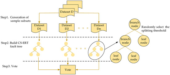
Figure 2.
Schematic diagram of the structure of a cost-sensitive extreme random forest.
In step2 in Figure 2, the fault tree node splitting process is shown. As CS-ERF is derived from ERF, it has the same randomness in the node splitting process and still consists of root, leaf, and branch nodes. If a node belongs to a branch node, a value is randomly selected in its sample as the splitting threshold for that node splitting, and the splitting of the node as above is performed. If it is a leaf node, then this node split ends and all values in it are categorized into the same sample class.
CS-ERF differs from ERF by changing the idea of entropy gradient descent to cost gradient descent, while the cost function of CS-ERF is designed as misclassification cost gain. When the node is split, analogous to extreme random forest, the misclassification cost of the node is defined in this paper, and the feature with the largest misclassification cost gain is specified as the splitting feature. For node misclassification, cost is defined as:
where C denotes the misclassification cost of a node, and and represent the cost of a node being in the fault and normal classes, respectively. and are calculated as in Equations (16) and (17), respectively.
where , , , and represent the number of samples incorrectly predicted as fault category, correctly predicted as fault category, incorrectly predicted as normal category, and correctly predicted as normal category, respectively, and according to the conclusion of Table 1, the values of and are 0, so Equations (18) and (19) can be obtained.
where and represent the total number of faulty and normal samples, respectively. A weighting factor is added to Equations (16) and (17), and the cost of correct categorization is 0, making the formula more concise.
For the cost function of CS-ERF, Equation (20) is the definition of the misclassification cost gain for feature m.
where is the misclassification cost of the parent node before splitting, is the misclassification cost of the left child node after splitting, is the misclassification cost of the right child node after splitting, and and are the number of samples in the left and right child nodes after splitting, respectively. It is easy to see that the coefficient before the misclassification cost of the child node is the weighting factor of the cost of the child node, and the misclassification cost of the parent node and its difference can obtain the misclassification cost gain of this node.
Due to the imbalance of samples in the transducer valve fault detection, the integrated algorithm used in the past tends to bias the results toward the sample class with a large number of samples when training the model, while the CS-ERF algorithm introduces a class distribution in the misclassification cost gain, thus allowing the model to care more about the fault class data with a very small number of samples, improving the accuracy of the algorithm and improving the detection performance of the model.
Combining the above studies, based on Bayes’ theorem, this paper determines that the class with the smallest misclassification cost function is the class of the corresponding leaf node, which is defined as follows:
where represents the posterior probability that sample x belongs to category . The CS-ERF in this paper solves the problems such as inaccurate results due to sample imbalance by adding the misclassification cost to the criterion at node splitting, thus achieving cost sensitivity.
Equation (22) is the construction of the objective function of the extreme random forest algorithm based on cost sensitivity.
where represents the misclassification cost, represents the canonical term, and N represents the total number of nodes.
When all base classifiers are finished running, the final sample class is decided using a minority–majority approach, as in Equation (23):
where represents the base classifier model, k represents the classification result of the base classifier, and I(∙) represents the exponential function. The final fault detection result of CS-ERF is obtained from the above equation.
4. Optimized CS-ERF Converter Valve Fault Detection
There are two common types of faults in the detection of converter valve faults: missing alarm rate (MAR) and false alarm rate (FAR). In the field of practical application, the impact of missed fault detection on production and life is far greater than that of the false detection of faults. When the CS-ERF algorithm in this paper is applied to the fault detection of the converter valve, the MAR can be well controlled at a lower level. Considering the complexity of the state parameters of the converter valve, operations such as data cleaning and feature selection should be performed on the data in the SCADA system before training the model.
4.1. Data Preprocessing
Due to the complex operation of the converter valve, the state quantities generated are also complex and there are more redundant variables, which will increase the complexity of model training and affect the prediction performance of the model. As shown in Figure 3, the data collected from the SCADA dataset are first cleaned, subjected to Pearson correlation analysis to remove redundant feature values, and then ranked by the importance of the feature values and feature selection. The Pearson correlation coefficient is calculated as the quotient of the covariance and standard deviation between two variables, as shown in Equation (24); through Pearson correlation analysis, some of the redundant features with low correlation are removed, making the model training more efficient and the prediction results more accurate.
where represents the correlation coefficient between features in the sample, represents the standard deviation of the corresponding features, and represents the covariance between features.
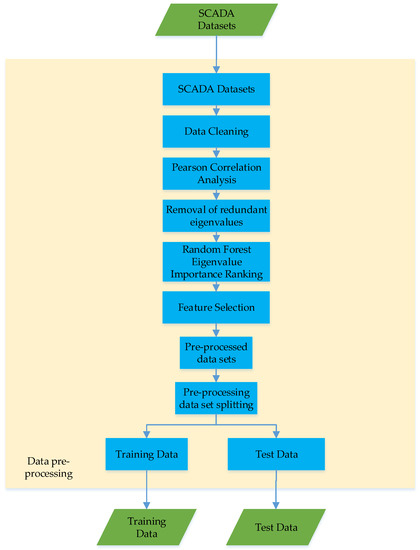
Figure 3.
Data preprocessing process.
Further, as the dataset often contains a large number of features, using random forest ranking, the features that contribute more to the results can be filtered out and the complexity of model training can be reduced. In this paper, the Gini index and variable importance (VI) are used as evaluation indicators to measure the contribution of each feature to the results, and the larger the contribution, the higher the importance. The Gini is calculated as:
The VI score of feature j is calculated as Equation (26):
where is the Gini coefficient, T represents the number of categories, represents the proportion of category t in node m, and represent the Gini index of two new nodes after node branching, n represents the tree, and M represents the set of features j appearing in decision tree i. In simple terms, it is the probability that two samples are arbitrarily drawn from node m and their categories do not agree.
After Pearson analysis and feature importance ranking, the dataset is divided into a training set and a test set. The training set is the data sample used for model fitting and training the classification model; the test set is used for model prediction, measuring the performance and classification ability of the model, and performing model prediction performance evaluation.
After data preprocessing, the CS-ERF fault detection model generation process is shown in Figure 4. The CS-ERF model parameters are obtained through the PSO optimization algorithm, and the fault detection model is jointly generated with the training data. Finally, the average misclassification cost (AMC) is selected; gMean, computing time, and missing alarm rate (MAR) are used as evaluation indicators. The performance of the test model is tested by using the real class labels of the test dataset and the predicted class labels generated by the model.
where TP, TN, FP, and FN represent the number of corresponding detected samples, and , , , and represent the corresponding misclassification cost parameters.
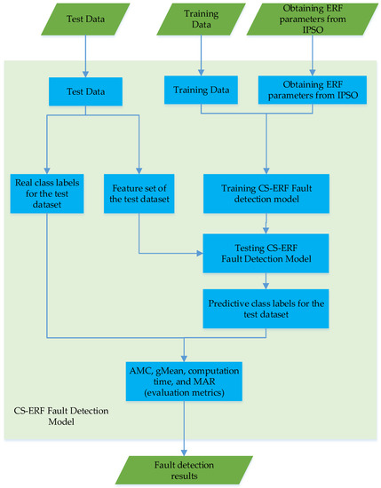
Figure 4.
CS-ERF fault detection model generation process.
4.2. Model Building Process
The fault detection flow chart of the CS-ERF converter valve based on the IPSO optimization algorithm is shown in Figure 5. After initializing the position and velocity of each particle to obtain the historical optimal position and historical optimal fitness value of individuals and groups, if the iterative conditions are satisfied, the parameters of the minimum misclassification cost of the CS-ERF model are output to obtain the best parameters needed for the fault diagnosis model to make the model work best [25,26]. If they are not satisfied, the speed and position of each particle, the historical optimal value, and the historical optimal fitness value of the group are updated until the iterative conditions are satisfied.
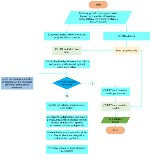
Figure 5.
Flow chart of CS-ERF converter valve fault detection based on IPSO.
The CS-ERF model has five hyperparameters, which are the two misclassification cost parameters , the maximum number of features, the minimum number of leaf nodes, and the number of decision trees M. Due to the large number of hyperparameters in the model, it is difficult to manually set the model. The best results are obtained, so the PSO algorithm is used to calculate the optimal hyperparameters.
In order to verify the superiority of the CS-ERF model under the PSO algorithm, after the data preprocessing of the dataset, this paper compares it with Moth-flame Optimization (MFO) [27], Multi-Verse Optimization (MVO) [28], Bat Optimization Algorithm, (BA) [29], Sparrow Search Algorithm (SSA) [30], and Particle Swarm Optimization (PSO). The model performance is evaluated and compared. The missed detection rate refers to the proportion of missed detection samples to the total samples during fault detection, and the gMean value refers to the square root of the product of the probability of correctly detecting faulty samples and the probability of correctly detecting normal samples. The lower the rate, the better the model performance and the shorter the running time. In order to prevent over-fitting and improve the accuracy of the model, each model is trained using ten-level cross-validation during comparative experiments.
5. Experimental Analysis
5.1. Data Description
This experiment selects the actual operation data of the converter valve in a converter station in China from June to December 2020. The converter valve is one of the most important devices in the DC transmission system, which determines the stability of the regional power grid to a certain extent. Its relatively complex fabrication process and critical role make its operation process very complex. The dataset collected in this paper includes a series of operational data in the thyristor assembly, valve cooling assembly, valve arrester, and external environment. The most important converter valve faults are IGBT device drive faults, IGBT device breakdown, communication faults, sub-module energy extraction power faults, and sub-module central control board faults.
As shown in Table 2, the dataset includes 1431 groups of data, among which 809 cases are in the normal state, 398 cases are in the attention state, 165 cases are in the abnormal state, and 59 cases are in the serious state. The above states are divided according to the number or severity of faults, and then the training set and test set are divided proportionally.
Table 2.
Data distribution.
5.2. Sample Feature Selection
Data pre-processing is performed on the above collected data, data cleaning is conducted to remove duplicate and redundant data screening, and the features whose state amount is always 0 are deleted. Pearson data analysis is used to delete the features with low correlation by calculating the correlation coefficient, and to keep the features with high correlation with the state of the converter valve. Based on the data samples at this time, the random forest importance ranking is used to calculate the comprehensive importance of the features, and the features with low importance ranking are deleted. Based on this data sample, the features with low importance ranking are deleted, and the remaining features are used as the main influencing factors of the state of the converter valve. The optimal feature set obtained after data pre-processing is shown in Table 3.
Table 3.
Data Optimum Solicitation.
5.3. Experimental Results
The MFO, MVO, BA, SSA, PSO, and IPSO optimization-seeking algorithms are brought into the flow chart of the converter valve failure model for the purpose of comparative analysis. By repeatedly testing different particle numbers, the number of particles that perform optimally at the moment of the results is recorded. The number of particles in the improved particle swarm optimization algorithm is set to 35, and ten trials are performed for all six optimization algorithms. After data pre-processing, the comprehensive performance of the six algorithms is evaluated using the missed detection rate (MAR), average misclassification cost (AMC), gMean, and running time as indicators, as shown in Figure 6.
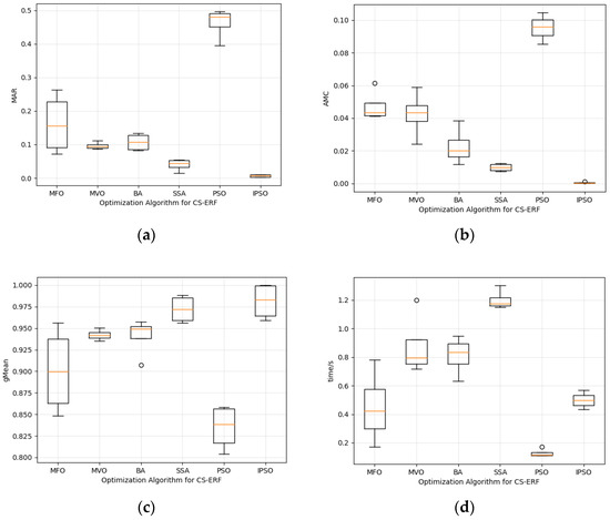
Figure 6.
(a) Comparison of the MAR of the six algorithms; (b) comparison of the AMC of the six algorithms; (c) comparison of the gMean values of the six algorithms; (d) comparison of the time used to run the six algorithms.
In Figure 6a, it is obvious that the model using the IPSO algorithm has the lowest miss detection rate, and the average miss detection rate of the IPSO is 0.68%, while the average miss detection rate of the other four algorithms is higher than 0.05, and the average MAR of PSO is 0.46 higher than that of IPSO. In Figure 6b, IPSO shows good parameter search performance, which makes CS-ERT have the lowest AMC of 0.04%, which is 0.0086 lower than that of the SSA algorithm that follows closely, and PSO is still worse than IPSO in this evaluation criterion. In Figure 6c, the IPSO algorithm achieves the highest gMean value, which represents the highest correct detection rate of the IPSO algorithm and the best performance, better than the first five algorithms. The average gMean value is 0.009 higher than that of the SSA algorithm, which is second to IPSO. In Figure 6d, it is clear that the IPSO algorithm outperforms the other four algorithms with an average runtime control of 0.49 s, while the slowest-running SSA algorithm has an average runtime of up to 1.2 s, indicating that the combination of IPSO and CS-ERF greatly improves the running speed of the model. Although IPSO does not take the fastest time, it stays within an acceptable range, and PSO, which takes the shortest time, takes an average of 0.12 s. Overall, IPSO has the best overall performance. Compared with the other five algorithms, the IPSO algorithm is less susceptible to noise, has the strongest integration performance and generalization ability, and can minimize model bias and improve fault detection performance by considering the misclassification cost of detection samples.
5.4. Limitations Discussion
For the model proposed in this paper, there are several limitations. First, although it outperforms the other five algorithms in MAR, AMC, and gMean, it is worse than the particle swarm optimization algorithm before improvement in terms of running time. When dealing with a large amount of high-dimensional complex data, the long running time will lead to excessive memory consumption, and the real-time performance of the model is not guaranteed and the computational cost is high. Second, the model proposed in this paper is more dependent on the data type, and data pre-processing must be performed in the early stage; otherwise, the detection accuracy of the model will be greatly reduced. Again, for unsupervised samples in the training dataset, cost-sensitive learning will encounter difficulties when the label information is unknown. Finally, in the gMean metric, the performance is optimal, but the performance of the results is not stable enough compared to the MVO algorithm, and the model stability needs to be improved.
6. Conclusions
To address the problems of unbalanced converter valve state data, difficult parameter selection, and poor performance of fault detection models, an UHV converter valve fault detection method based on optimization cost-sensitive extreme random forest is proposed.
The contributions of this paper are mainly fourfold. First, the adaptive inertia factor as well as the learning factor, which can be dynamically adjusted during the iterative process, are proposed to be incorporated into the position and velocity update formulas to construct an IPSO to find the optimal hyperparameters of the model. The IPSO is less likely to fall into the local optimum, the search efficiency is improved, the convergence speed is fast, and the overall optimization-seeking capability is improved. Second, Pearson correlation analysis and random forest feature importance ranking are used in data preprocessing for data cleaning to remove redundant features and retain the most helpful features for detection results. Again, the misclassification cost gain is introduced into the extreme random forest as the classification index of the fault tree to solve the influence of unbalanced data on the detection results, and the cost-sensitive extreme random forest is constructed to improve the comprehensive performance of the model fault detection. Finally, an IPSO is used to find the optimal hyperparameters of the model to achieve fast response of the model and high classification accuracy, good robustness, and generalization under unbalanced data.
In this paper, four metrics are introduced to optimize the CS-ERF using six optimization algorithms, MFO, MVO, BA, SSA, PSO, and IPSO, and the results show that the model has a more excellent detection performance when optimized using IPSO. Based on the proposed UHV converter valve fault diagnosis based on improved optimization cost-sensitive extreme random forest, the following shows suggestions for future research:
- With the technical upgrade of the transmission system, the dimensionality and complexity of the features contained in the original dataset grow rapidly, different data pre-processing methods of model evaluation will have a large impact, and the data pre-processing methods that are more suitable for this paper can be further studied.
- The particle swarm optimization algorithm can be combined with other optimization algorithms to build a new location iteration method, which makes the model optimal hyperparameters more accurate and improves the accuracy of model detection.
- The proposed method can be applied to other fault detection fields.
Author Contributions
Supervision, F.X.; writing—original draft, C.C.; formal analysis, M.T.; investigation, Z.W.; data curation, J.T.; conceptualization, J.Y. All authors have read and agreed to the published version of the manuscript.
Funding
This work was supported in part by the Science and Technology Project of State Grid Hunan Electric Power Co., Ltd. (grant no. 5216A3210013), the National Natural Science Foundation of China (grant no. 62173050), the Energy Conservation and Emission Reduction Hunan University Student Innovation and Entrepreneurship Education Center, and the Graduate Scientific Research Innovation Project of Changsha University of Science and Technology (grant no. CXCLY2022094).
Data Availability Statement
The data that support the findings of this study are available from the corresponding author upon reasonable request.
Conflicts of Interest
The funder had the following involvement with the study: supervision, formal analysis, and investigation. The authors declare no conflict of interest.
References
- Alassi, A.; Bañales, S.; Ellabban, O.; Adam, G.; MacIver, C. HVDC Transmission: Technology Review, Market Trends and Future Outlook. Renew. Sustain. Energy Rev. 2019, 112, 530–554. [Google Scholar] [CrossRef]
- Lu, J.; Yuan, X.; Zhang, M.; Hu, J. Supplementary Control for Mitigation of Successive Commutation Failures Considering the Influence of PLL Dynamics in LCC-HVDC Systems. CSEE J. Power Energy Syst. 2022, 8, 872–879. [Google Scholar]
- Jiang, T.; Yu, Y.; Jahanger, A.; Balsalobre-Lorente, D. Structural emissions reduction of China’s power and heating industry under the goal of “double carbon”: A perspective from input-output analysis. Sustain. Prod. Consum. 2022, 31, 346–356. [Google Scholar] [CrossRef]
- Mehdi, A.; Kim, C.-H.; Hussain, A.; Kim, J.-S.; Hassan, S.J.U. A Comprehensive Review of Auto-Reclosing Schemes in AC, DC, and Hybrid (AC/DC) Transmission Lines. IEEE Access 2021, 9, 74325–74342. [Google Scholar] [CrossRef]
- National Grid Co. Guidelines for Condition Evaluation of High Voltage DC Transmission Converter Valves; China Electric Power Publishing House: Beijing, China, 2011. [Google Scholar]
- Mei, F.; Li, X.; Zheng, J.; Sha, H.; Li, D. A data-driven approach to state assessment of the converter valve based on oversampling and Shapley additive explanations. IET Gener. Transm. Distrib. 2022, 16, 1607–1619. [Google Scholar] [CrossRef]
- Li, F.; Shi, P.; Lim, C.-C.; Wu, L. Fault Detection Filtering for Nonhomogeneous Markovian Jump Systems via a Fuzzy Approach. IEEE Trans. Fuzzy Syst. 2016, 26, 131–141. [Google Scholar] [CrossRef]
- Zhang, S.; Lang, Z.-Q. SCADA-data-based wind turbine fault detection: A dynamic model sensor method. Control Eng. Pract. 2020, 102, 104546. [Google Scholar] [CrossRef]
- Badihi, H.; Zhang, Y.; Jiang, B.; Pillay, P.; Rakheja, S. A Comprehensive Review on Signal-Based and Model-Based Condition Monitoring of Wind Turbines: Fault Diagnosis and Lifetime Prognosis. Proc. IEEE 2022, 110, 754–806. [Google Scholar] [CrossRef]
- Zhang, D.; Qian, L.; Mao, B.; Huang, C.; Huang, B.; Si, Y. A Data-Driven Design for Fault Detection of Wind Turbines Using Random Forests and XGboost. IEEE Access 2018, 6, 21020–21031. [Google Scholar] [CrossRef]
- Hussain, A.; Kim, C.; Admasie, S. An intelligent islanding detection of distribution networks with synchronous machine DG using ensemble learning and canonical methods. IET Gener. Transm. Distrib. 2021, 15, 3242–3255. [Google Scholar] [CrossRef]
- Chen, Z.; Liu, C.; Ding, S.X.; Peng, T.; Yang, C.; Gui, W.; Shardt, Y.A.W. A Just-In-Time-Learning-Aided Canonical Correlation Analysis Method for Multimode Process Monitoring and Fault Detection. IEEE Trans. Ind. Electron. 2020, 68, 5259–5270. [Google Scholar] [CrossRef]
- Qin, Y.; Yan, Y.; Ji, H.; Wang, Y. Recursive Correlative Statistical Analysis Method With Sliding Windows for Incipient Fault Detection. IEEE Trans. Ind. Electron. 2021, 69, 4185–4194. [Google Scholar] [CrossRef]
- Khan, S.H.; Hayat, M.; Bennamoun, M.; Sohel, F.A.; Togneri, R. Cost-Sensitive Learning of Deep Feature Representations From Imbalanced Data. IEEE Trans. Neural Netw. Learn. Syst. 2018, 29, 3573–3587. [Google Scholar] [CrossRef]
- Jing, X.-Y.; Zhang, X.; Zhu, X.; Wu, F.; You, X.; Gao, Y.; Shan, S.; Yang, J.-Y. Multiset Feature Learning for Highly Imbalanced Data Classification. IEEE Trans. Pattern Anal. Mach. Intell. 2019, 43, 139–156. [Google Scholar] [CrossRef]
- Zhu, X.; Yang, J.; Zhang, C.; Zhang, S. Efficient Utilization of Missing Data in Cost-Sensitive Learning. IEEE Trans. Knowl. Data Eng. 2019, 33, 2425–2436. [Google Scholar] [CrossRef]
- Li, W.; Wang, G.-G.; Gandomi, A.H. A Survey of Learning-Based Intelligent Optimization Algorithms. Arch. Comput. Methods Eng. 2021, 28, 3781–3799. [Google Scholar] [CrossRef]
- Wang, D.; Tan, D.; Liu, L. Particle swarm optimization algorithm: An overview. Soft Comput. 2018, 22, 387–408. [Google Scholar] [CrossRef]
- Wang, Z.-J.; Zhan, Z.-H.; Kwong, S.; Jin, H.; Zhang, J. Adaptive Granularity Learning Distributed Particle Swarm Optimization for Large-Scale Optimization. IEEE Trans. Cybern. 2020, 51, 1175–1188. [Google Scholar] [CrossRef]
- Liu, W.; Wang, Z.; Yuan, Y.; Zeng, N.; Hone, K.; Liu, X. A Novel Sigmoid-Function-Based Adaptive Weighted Particle Swarm Optimizer. IEEE Trans. Cybern. 2019, 51, 1085–1093. [Google Scholar] [CrossRef]
- Wen, L.; Xu, M.; Jiao, J.; Wu, T.; Tang, M.; Cai, S. A velocity-based butterfly optimization algorithm for high-dimensional optimization and feature selection. Expert Syst. Appl. 2022, 201, 117217. [Google Scholar]
- Tang, M.; Yi, J.; Wu, H.; Wang, Z. Fault Detection of Wind Turbine Electric Pitch System Based on IGWO-ERF. Sensors 2021, 21, 6215. [Google Scholar] [CrossRef] [PubMed]
- Tang, M.; Cao, C.; Wu, H.; Zhu, H.; Tang, J.; Peng, Z. Fault Detection of Wind Turbine Gearboxes Based on IBOA-ERF. Sensors 2022, 22, 6826. [Google Scholar] [CrossRef] [PubMed]
- Chicco, D.; Jurman, G. The advantages of the Matthews correlation coefficient (MCC) over F1 score and accuracy in binary classification evaluation. BMC Genom. 2020, 21, 6. [Google Scholar] [CrossRef] [PubMed]
- Long, W.; Jiao, J.; Liang, X.; Wu, T.; Xu, M.; Cai, S. Pinhole-imaging-based learning butterfly optimization algorithm for global optimization and feature selection. Appl. Soft Comput. 2021, 103, 107146. [Google Scholar] [CrossRef]
- Long, W.; Jiao, J.; Liang, X.; Xu, M.; Tang, M.; Cai, S. Parameters estimation of photovoltaic models using a novel hybrid seagull optimization algorithm. Energy 2022, 249, 123760. [Google Scholar] [CrossRef]
- Khan, M.; Sharif, M.; Akram, T.; Damaševičius, R.; Maskeliūnas, R. Skin Lesion Segmentation and Multiclass Classification Using Deep Learning Features and Improved Moth Flame Optimization. Diagnostics 2021, 11, 811. [Google Scholar] [CrossRef]
- Abualigah, L. Multi-verse optimizer algorithm: A comprehensive survey of its results, variants, and applications. Neural Comput. Appl. 2020, 32, 12381–12401. [Google Scholar] [CrossRef]
- Yu, H.; Zhao, N.; Wang, P.; Chen, H.; Li, C. Chaos-enhanced synchronized bat optimizer. Appl. Math. Model. 2019, 77, 1201–1215. [Google Scholar] [CrossRef]
- Zhang, C.; Ding, S. A stochastic configuration network based on chaotic sparrow search algorithm. Knowl.-Based Syst. 2021, 220, 106924. [Google Scholar] [CrossRef]


Publisher’s Note: MDPI stays neutral with regard to jurisdictional claims in published maps and institutional affiliations. |
© 2022 by the authors. Licensee MDPI, Basel, Switzerland. This article is an open access article distributed under the terms and conditions of the Creative Commons Attribution (CC BY) license (https://creativecommons.org/licenses/by/4.0/).