Optimizing Operation Strategy in a Simulated High-Proportion Wind Power Wind–Coal Combined Base Load Power Generation System under Multiple Scenes

Abstract

In order to accommodate more intermittent renewable energy in coal-dominated power systems, conventional thermal power plants need to improve their operational flexibility to balance the energy system at all times. However, flexible operation of coal-fired power plants could reduce energy efficiency and increase CO₂ and pollutant emission, so it is important to consider environmental implications and optimize the dispatch of wind and coal power units in the system. In this paper, based on the output profile of wind power, a wind power peak (T, H) simulation model based on Gaussian distribution was established. Using a high-proportion wind power wind–coal combined base load power generation system as an example, the economical and environmentally friendly unit operation based on different wind power penetration was studied by simulation, and the decision strategy was established. Wind energy curtailment boundary was determined with power generation cost, energy consumption, CO₂ and pollutant emissions as decision targets, respectively. Weekly scale results indicate that incorporating energy consumption and pollutant emissions into consideration will lead to different decision-making strategies compared with only targeting minimizing wind curtailment. This paper established a decision-making model of wind–coal system operation strategy based on economy and environmental criteria. This work directly contributes to real system operation and is of great significance for future scheduling/dispatch studies of actual power systems.

1. Introduction

1.1. Background

China has proposed an ambitious plan for renewable energy development [1,2,3,4]. The goal is to achieve 20% of non-fossil energy production by 2030. This target will be mainly achieved by increasing utilization of wind and solar energy [5,6,7]. With strong support from the government, renewable power generation has developed rapidly in the past decade. By the end of 2016, China has become the world’s largest country in wind power and solar power installed capacity. Due to the intermittency of wind and solar power generation, large-scale integration of wind and solar power onto the grid requires conventional thermal power plants to balance the load.

China’s power supply structure is still dominated by coal-fired power with only a very small share from flexible sources, such as natural gas and pumped-storage hydropower. In the three northern regions of China (North China, Northwest China, Northeast China), wind power and solar power generation account for a large share, and the task of load balancing is mainly performed by coal-fired power units. Although wind and solar power can be considered as zero emissions, their intermittent and uncertain outputs could increase the economic costs and pollutant emissions from coal power units in the system. As wind power capacity increases, the thermal power units in the network need to operate with more flexibility (including frequent deep cycling, frequent start-up and shutdown), which would increase coal consumption and emissions accordingly [8,9,10,11,12,13,14]. Recently, researchers have been focusing on system dispatch and scheduling models of power systems with high wind power penetration. Yang et al. [15] used a simulation method to build a dispatch model that could strengthen wind power absorption, ensure secure operation, and improve the robustness of the dispatch strategy. Li et al. [16] also purposed a scheduling model that could reduce the operation costs and impact of wind power uncertainty for a district integrated natural gas and power system.

Some studies have examined the economic and environmental impacts of renewable power integration with thermal power generation, but most have focused on U.S. power systems [9,17]. Frade et al. [18] studied the wind balancing cost in a power system with high wind penetration in Portugal. Study [19] used operational data from two typical coal power plants in China (300 MW and 600 MW) to analyze coal consumption and emission characteristics at different output levels and during the start-up process. There are some studies on energy efficiency and emission characteristics of energy systems with renewable penetration [10,12], but they are mainly focused on energy systems of specific regions. The literature [20] modeled and analyzed the energy efficiency, CO₂ and pollutant emission characteristics of typical wind–coal combined systems in Northeast China, but it did not include a dispatch strategy for the system.

1.2. Literature Review

At present, the research on high-penetration wind–coal combination power generation systems mainly focus on how to improve the wind power accommodation through the flexible operation of coal-fired units. For example, the study [21] gives a method to improve the flexibility of coal-fired units through flexible fuel switching, and literature [22] studies the method of improving the flexibility of the unit through fast start–stop technology. The studies [23,24,25] research the technology for improving the operational flexibility of coal-fired units through optimizing control systems, and the method of improving the flexibility of the unit through thermal energy storage and chemical energy storage is listed in [26,27,28].

In wind–coal combined power generation system dispatching, the current research focuses on the combined economic emission dispatch (CEED) problem, which takes both economic and environmental protection into consideration. The report [29] gives a detailed review of this issue. The research on CEED problem mainly focuses on optimization algorithms, which can be divided into three categories, which are traditional methods, non-traditional methods and hybrid methods. Traditional methods include goal programming [30], linear programming [31], Newton-Raphson [32], evolutionary programming [33], stochastic search techniques [34]. Non-traditional methods include the genetic algorithm [35], particle swarm optimization [36], simulated annealing [37], firefly algorithm [38], artificial bee colony [39], bat algorithm [40], etc. Mixing methods are the DE-CRO [41], DE-SA [42], FFA-GA [43], DE-HS [44], BF-NM [45], PSO-GA [46], PSO-GSA [47], metaheuristic [48], etc. These works usually only use the energy consumption and pollutant emission functions in the normal peak shaving range of the generators in the system and establish a comprehensive single-objective or multi-objective optimization function to solve the problem. However, the optimal unit input problem and the implication of flexibility operation (ultra-low load, load ramping, and startup-shutdown) on energy consumption and pollutant emission are rarely considered. The study [49] considers the influence of unit flexibility and determines the optimal wind power consumption level through optimization calculations, but does not give a clear wind power curtailment boundary.

To the best of our knowledge, the literature on the optimization of the operation strategy of the wind–coal combined power generation system mainly focuses on the optimization objective function, such as the least wind power abandonment, the lowest power generation cost, the lowest pollutant emission, etc., and uses advanced and efficient solution algorithm to optimize the unit combination or scheduling. Then, the optimal unit start–stop strategy and optimal unit load distribution at each time period are determined.

However, this paper focuses on the research concerning the wind curtailment boundary and the operation strategy of a high-proportion wind power wind-coal combined base load power generation system, with the premise of a flexible operation of coal-fired power units. The wind curtailment boundary (T, H) under different decision goals (net profit, net coal consumption reduction, net emission reduction of CO₂ and net emission reduction of NO_x) were obtained using a simulation method. The optimal unit operation strategy of each decision point was determined through the operation decision of the power generation system with the actual wind power curve.

Accurate power generation cost models, pollutant emission models and reasonable unit input decision are the basis of optimal dispatch of wind–coal power generation system. Therefore, based on wind power peak simulations using Gaussian distribution, a unit operation strategy decision model was established, and the research on decision-making of the wind power curtailment boundary and optimal unit input combination under different decision-making objections was subsequently carried out.

1.3. Research Contribution

The power transmission of large-scale wind power bases requires a certain proportion of coal-fired power units as support. When a wind–coal combined power system operation with high-proportion wind power, the intermittency and fluctuation of wind power requires coal-fired units to operate more flexibly. The flexible operation of coal-fired units (including low minimum load, fast start-up and shutdown, high ramp rates) usually leads to the unwanted increase in costs and emissions of carbon and other pollutants. Therefore, it is necessary to investigate the optimization investment and wind energy curtailment boundary decisions of wind–coal combined systems, taking the economic and environmental impact of coal-fired power units in flexible operation conditions into consideration.

The contributions of this paper are summarized as below:

(1)

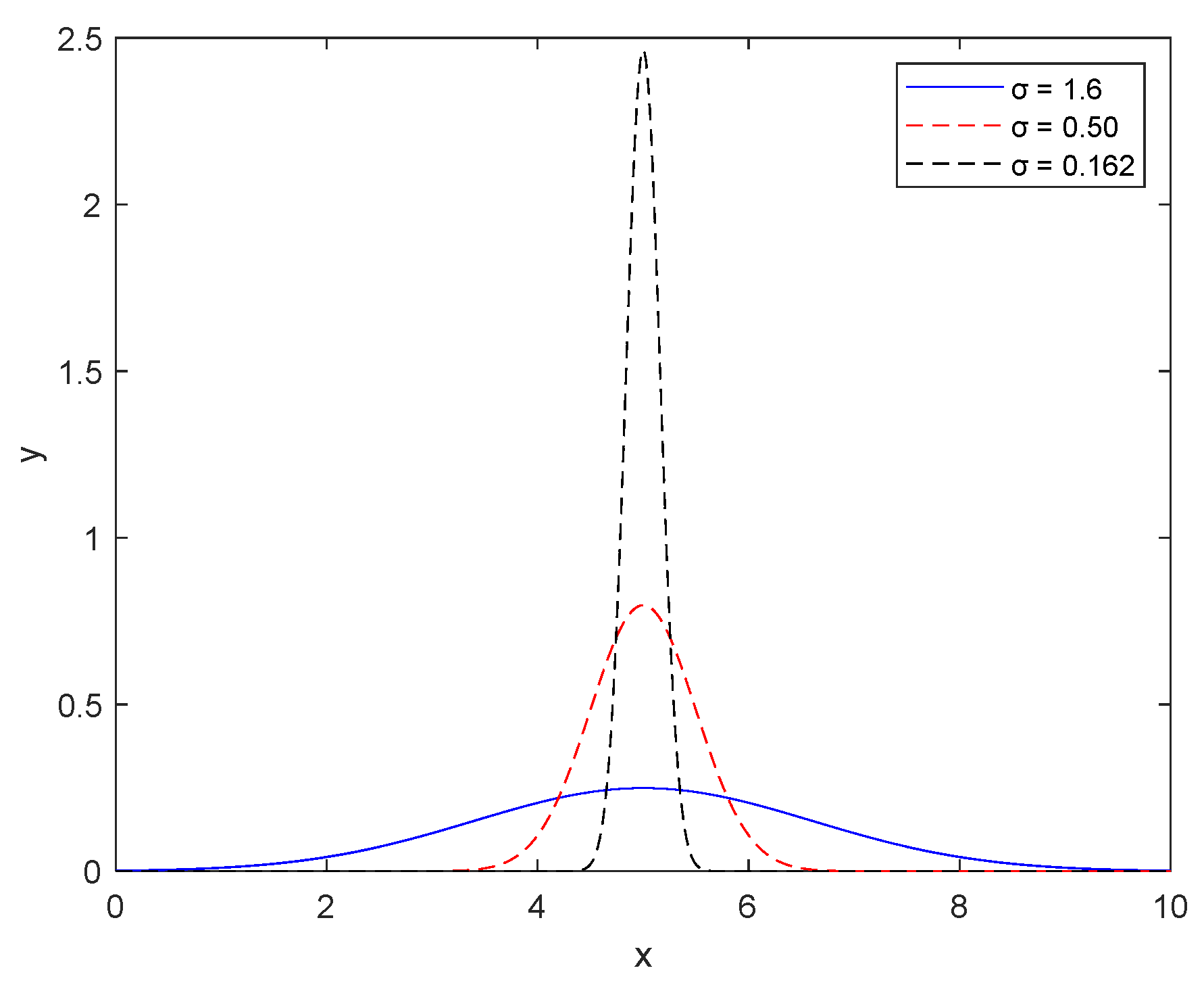
A simulation model of the peak of the wind power curve was established based on the Gaussian distribution, which can simulate the peaks of different shapes, aiming at the peak characteristics of the power curve of the wind farm;

(2)

A decision-making model for unit operation strategy based on economic and environmental considerations was established, by researching the base load wind–coal combined power generation system with a high-proportion of wind power;

(3)

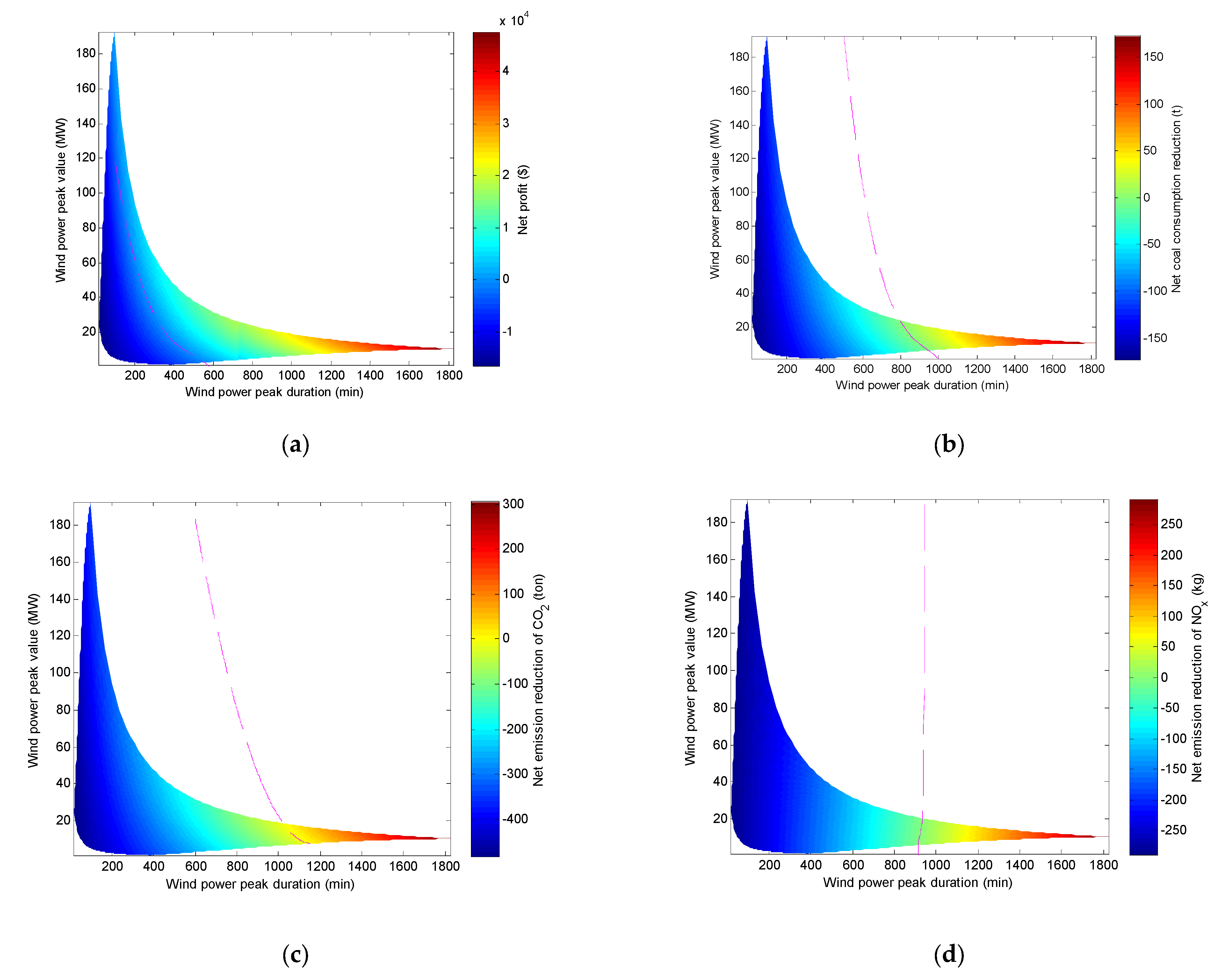
The wind energy curtailment boundary with power generation costs, energy consumption, CO₂ and pollutant emissions as the decision-making targets was determined based on simulations of wind power peaks on the base load wind–coal combined power generation system;

(4)

For the wind–coal combined base load power generation system based on the actual wind power curve, the optimal investment combination decision on the weekly scale unit was studied, and the optimal combination decision of the unit was achieved.

2. Wind Power Peak Curve Simulation Model

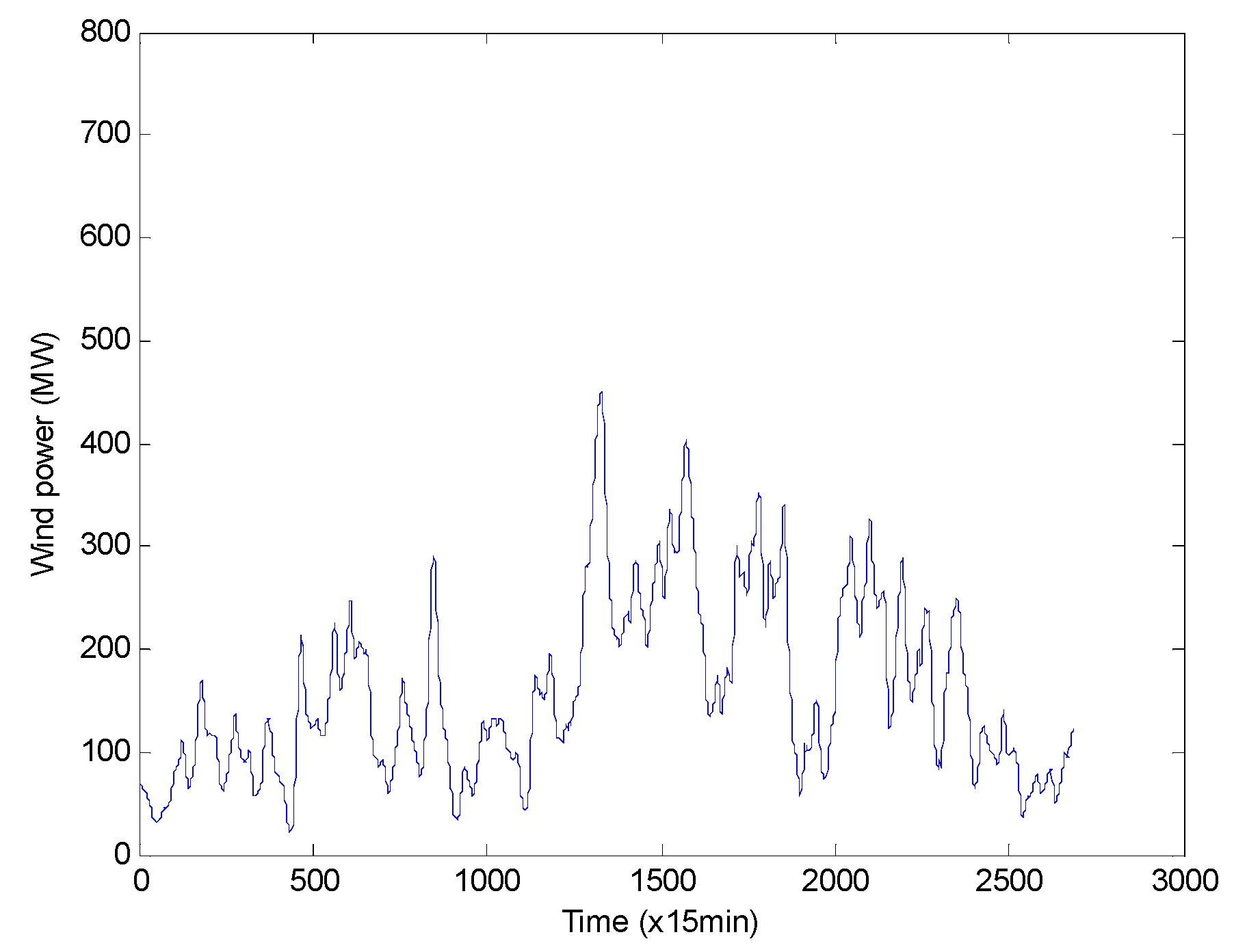
2.1. Analysis of Wind Power Peak Characteristics

Taking a regional wind farm (17 × 49.5 MW) as an example, the theoretical wind power curve for one month is shown in Figure 1, and for one week in Figure 2.

It can be seen from Figure 1 that the total wind power of the month varies greatly (between 40 MW and 450 MW), but the power change rate is relatively small, which is mainly due to the complementary action of different regional wind power units and wind farms [2]. The entire wind power curve can be seen as consisting of a series of peaks and valleys, and the shape parameters of the peaks and valleys directly affects the operating strategy of the entire wind–coal combined power generation system.

The wind power data of the second week of the month is shown in Figure 2 of the paper. It can be seen that the shape of the curve peak can be roughly divided into three categories: “steep”, “smooth” and “flat”, as shown in peak ①, ② and ③, respectively. The “steep” wind power peaks indicates that the average wind power change rate is large during this period. Under the operation strategy of not abandoning wind power, the coal-fired power unit needs to be complemented by a rapid load change or rapid start–stop, which may bring additional cost. The “flat” wind power peaks means that the average wind power change rate is small during this period, usually complementary coal-fired power units can meet the system load requirements through normal output adjustment. The “smooth” wind power peaks mean the internal average wind power change rate in this period is between the former two. The shape of the wave crest can be described by two parameters, the width T and height H of the wave peak. A large H/T corresponds to a “steep” wind power peak; a small H/T corresponds to a “flat” wind power peak. Using the statistical analysis of the power data of the wind power system in this region throughout a year, it is found that the average wind power change rate (slope) of the peak is within 3 MW/min.

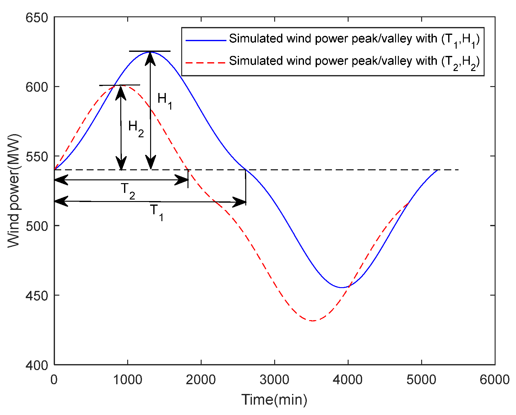
2.2. Simulation of Power Peak Curve of Wind Farm Based on Gaussian Distribution

Based on the above analysis, this paper used Gaussian distribution to simulate the wind power peak curve of a wind power system. The single parameter Gaussian distribution function is as follow [50]:

$$f\left(x\right)=\frac{1}{\sqrt{2\pi }\sigma }{e}^{-\frac{{\left(x-\mu \right)}^2}{2{\sigma }^2}},x\in \left(-\infty ,+\infty \right)$$

(1)

where μ and σ are parameters, μ determines the position of the function curve, and σ determines the shape of the curve (short/slim). Different wind power curve peaks can be simulated using different σ values, as shown in Figure 3.

According to the Gaussian distribution 3σ principle, the area between the curve and horizontal axis is 99.74% in interval (μ − 3σ, μ + 3σ), so interval (μ − 3σ, μ + 3σ) can be regarded as the effective range of x. Value range. Within this interval, the average slope of peak curve can be approximated by the following equation.

$$k=\frac{1}{3\sqrt{2\pi }{\sigma }^2}$$

(2)

Generally, 1 min of active power change and 10 min of active power change are counted. In the process of grid-connection and wind speed growth, the active power change of the wind farm should meet the requirements of safe and stable operation of the power grid. The active power change limit should be determined by the power system dispatching institution according to the frequency modulation characteristics of the connected power grid.

The recommended values for the active power variation limit of the wind farm are shown in

Table 1. Wind farm active power change limit recommended value [51].

Wind Farm Installed Capacity (MW)	10 min Active Power Variation Upper Limit (MW)	1 min Active Power Variation Upper Limit (MW)
<30	10	3
30~150	Installed capacity/3	Installed capacity/10
>150	50	15

. This requirement can also be applied to normal shutdown of a wind farm. However, in special situations, such as wind speed decreasing or exceeding the cut-out speed, it is allowed to operate beyond the recommended values.

Using Formula (2), the Gaussian distribution function parameter σ can be taken as 1.6, 0.5, and 0.162, and the corresponding slopes of the curves are 0.052, 0.532, and 5.067, respectively. If power (MW) is represented by the y-axis and time (min) is represented by the x-axis, and the y-axis and x-axis are simultaneously expanded by the same multiple, different wind power peak curves can be simulated. Taking σ = 1.62 as an example, the simulated wind power peak curve is shown as Figure 4. It can be seen that the simulated wind power peak curve can be described by two characteristic parameters of width T and height H.

The capacity of wind power during the time period T₁ (the area under the wind power curve) can be calculated by the following formula:

$$P_{wind}=P\left(0\le T\le 2T_1\right)={\displaystyle {\int }_0^{2T_1}f\left(T\right)dT}$$

(3)

3. Operation Strategy Decision Model of Wind–Coal Combined Power Generation System

3.1. Brief Introduction of Wind–Coal Combined Power Generation System

The high-proportion wind power wind–coal combined base load power generation system consists of two types of power sources: wind power and coal-fired power. The wind power comprises 17 wind farms. The installed capacity of a single wind farm is 49.5 MW (1.5 MW × 33 units). The coal-fired power includes one sub-critical 300 MW unit and one sub-critical 600 MW unit, which are main peak shaving units in China. The power system has a basic load of 840 MW and is supplied by wind turbines (using wind farm theoretical wind power as wind power output) and coal-fired units. The upper limit of coal power output is 840 MW, and the lower limit is 105 MW. We chose this arrangement as the typical system being studied because according to the “14th Five-Year Plan” of the Chinese government, renewable power generation in most of the energy bases in Western China will account for more than 50% of the total installed capacity. Therefore, it is of great significance to study optimal operation strategies of power systems with a high proportion of renewable energy to ensure the safety and economic operation. According to this requirement, this paper selected a medium-sized wind power base (840 MW) and a coal-fired power unit (900 MW) with similar capacities to build a regional power system, and conducted research on the optimized operation strategy of a wind–coal combined system under different wind power output characteristic scenarios.

3.2. Operational Strategy

In a wind–coal combined base load power generation system; the operating strategy of coal-fired units needs to be considered under certain operating conditions. Taking the 840 MW wind–coal combined base load power generation system as an example, Figure 5 show the wind power curve and the complementary coal-fired power curve for a certain week. The operational strategy decision problem can be roughly divided into the following two scenarios. One is the combined economic and emission decision of optimal coal-fired unit commitment at a certain load when met with wind power peak, point “a” in Figure 5. The other is wind power curtailment (reduce some wind turbine’s power output or shutdown some wind turbines) or coal-fired unit shutdown decision when the predicted wind power peak occurs and complementary coal-fired power load is lower than the minimum safe power output, point “d” in Figure 5.

Operation strategies of the 840 MW wind–coal combined base load power system are listed in

Table 2. Operation strategies of the 840 MW wind–coal combined base load power generation system.

No.	Theory Wind Power (MW)	Coal-Fired Power (MW)	Coal-Fired Units Input Strategy 1	Coal-Fired Units Input Strategy 2
1	0~240	600~840	600 MW + 300 MW
2	240~540	300~600	600 MW + 300 MW	600 MW
3	540~630	210–300	300 MW	600 MW
4	630~735	105~210	300 MW

.

3.3. Unit Operation Strategy Decision Model

3.3.1. Wind Power Simulation of Wind Power Curve

According to Section 3.2, in the range of 0.162~1.6, σ can meet the requirements of the recommended value of the active power variation limit of the wind farm (Table 1). Here, the interval of 0.162–1.6 is divided into 99 parts, the interval point values are assigned to ${\sigma }_1,{\sigma }_2,\cdots ,{\sigma }_{100}$ in sequence, and different Gaussian distribution curves can be generated using different σ. For each independent Gaussian distribution curve, the interval [0.5σ, 3σ] is equally divided into 99 points, and the value of each interval point is twice the width of the peak curve, as shown by T₁ and T₂ in Figure 4. Hence, we simulated a matrix of 100 × 100, as shown in Formula (4).

$$\left[\begin{array}{ccc}0.5{\sigma }_1& \cdots & 0.5{\sigma }_{100}\\ ⋮& \ddots & ⋮\\ 3{\sigma }_1& \cdots & 3{\sigma }_{100}\end{array}\right]$$

(4)

Each element in the matrix represents the width of the peak, and the peak corresponding to each column element has approximately the same shape (slope). Finally, by multiplying the horizontal and vertical coordinates of different shapes and different widths by the same multiple, different wind power peaks can be simulated.

3.3.2. Unit Operation Decision Model

Unit Operation Decision Criterion

Under base load, when the wind power changes with time, the complementary coal-fired power should change accordingly. In low-load conditions, the coal consumption and air emission characteristics of the coal-fired power units will change greatly, and even the safe operation of the units will be jeopardized. Therefore, it is necessary to make a decision on the input unit combination, to obtain the optimal unit input. Under the premise of safe operation of the system, the decision criteria for the unit operation combination method can be divided into economic criteria, environmental protection criteria and economic environmental protection criteria.

(1)

Economic criteria

The variation of unit input operation combination would cause changes in power generation costs, including fuel costs and start-up costs.

The power generation cost characteristics of the unit are usually based on the secondary coal consumption characteristics (b-P_el curve) of the previously obtained unit, i.e., for calculating the fuel cost, the previously obtained coal consumption characteristics [16] are used, which is

$$b_n^s=a+b\times P_{el}+c\times P_{el}{}^2$$

(5)

where, $b_n^s$ is the standard coal consumption rate, kg/(kW·h); $P_{el}$ is active power, kW; and a, b and c are coefficients.

Then, the fuel cost characteristic (F-P curve) can be determined based on fuel price.

During start-up, steam turbine pipe warming, boiler temperature and pressure rising will consume energy, and increase power generation costs as a result.

There are two types of unit start-up cost models. One is cold state start cost model [52]:

$$F_s\left(\tau \right)=F_0\left(1-e^{-\tau /\alpha }\right)+F_i$$

(6)

where, the cold state start cost is determined by the initial cost of the boiler thermal inertia; $\alpha$ is the thermal time constant of the unit; $\tau$ is the number of hours of downtime for the unit; and $F_i$ is the fixed cost, mainly determined by the energy consumed by the turbine start-up and the operating personnel costs.

The other cost model corresponds to the hot start, expressed by the linear function, i.e.,

$$F_s\left(\tau \right)=F_0^{\prime }\tau +F_i$$

(7)

In the formula, $F_0^{\prime }$ is the starting cost required after one hour’s banked fire.

Operation strategy: Wind energy curtailment, and no coal-fired units are shutdown.

$$F_{\mathrm{mod}e1}=C_{\mathit{coal}}(T\cdot b_n^s\cdot P_{\mathit{el}}+\lambda {\displaystyle \sum _{i=1}^T{P}_{\mathit{eli}}})$$

(8)

In which, λ is the cost coefficient of wind energy curtailment, also called the penalty factor, 0.344 t/MW·h.

Operation strategy 2: No wind energy curtailment and only one coal-fired unit is shutdown.

$$F_{\mathrm{mod}e2}=C_{\mathit{coal}}\cdot {\displaystyle \sum _{i=1}^T(b_{ni}^s\cdot P_{\mathit{eli}}})+F_s$$

(9)

The net profit of strategy 2 relative to strategy 1 can be calculated as follows:

$$\Delta N_{\mathrm{net}2-1}=F_{\mathrm{mod}e1}-F_{\mathrm{mod}e2}$$

(10)

(2)

Environmental criteria

Operation strategy 1: Wind energy curtailment, and no coal-fired units are shutdown.

$$E_{\mathrm{mod}e1}={\displaystyle \sum _{i=1}^T{e}_i}{P}_{\mathit{eli}}$$

(11)

Operation strategy 2: No wind energy curtailment and only one coal-fired unit is shutdown.

$$E_{\mathrm{mod}e2}={\displaystyle \sum _{i=1}^T(e_i\cdot P_{\mathit{eli}}})+E_s$$

(12)

where, $E_{\mathrm{mod}e1}$ is the total air pollutant emissions under operation strategy 1, kg; $E_{\mathrm{mod}e2}$ is the total air pollutant emissions under operation strategy 2, kg; $e_i$ is the emission intensity of the ith air pollutant emission at active power $P_{\mathrm{el}i}$, g/(kW·h); $P_{\mathrm{el}i}$ is the active power of the coal-fired unit, kW; E_s is the starting emission of certain air pollutant emissions from the unit, kg.

The net air pollutant emission reduction of operational strategy 2 relative to strategy 1 is

$$\Delta E_{\mathrm{net}2-1}=E_{\mathrm{mod}e1}-E_{\mathrm{mod}e2}$$

(13)

Coal-Fired Unit Operation Decision against a Wind Power Peak above 540 MW

For a wind power peak above 540 MW, the operation strategies of a coal-fired unit can be

(1)

Wind energy curtailment: a 300 MW and 600 MW unit operate together;

(2)

Without wind energy curtailment: a 300 MW unit undergoes shutdown and a 600 MW unit remains operational;

(3)

Without wind energy curtailment: a 600 MW unit undergoes shutdown and a 300 MW unit remains operational.

For the three operation strategies, the decision criteria are as follows:

Decision criterion a: if ΔN_net2-1 < 0 then wind energy is curtailed or if ΔE_net2-1 < 0 then wind energy is curtailed;

Decision criterion b: if ΔN_net3-1 < 0 then wind energy is curtailed or if ΔE_net3-1 < 0 then wind energy is curtailed.

In which, $\Delta N_{\mathrm{net}3-1}$ and $\Delta E_{\mathrm{net}3-1}$ are the net profit and the net air pollutant emission reduction of operational strategy (3) relative to strategy (1) separately.

Coal-Fired Unit Operation Decisions against a Wind Power Peak above 240 MW

For wind power peak above 240 MW, the operation strategies of coal-fired unit can be:

(1)

Wind energy curtailment: a 300 MW and 600 MW unit operate together;

(2)

Without wind energy curtailment: a 300 MW and 600 MW unit operate at a reduced load;

(3)

Without wind energy curtailment: a 300 MW unit undergoes shutdown and a 600 MW unit remains operational.

For the three operation strategies, the decision criteria are as follows:

Decision criterion a: if ΔN_net2-1 < 0 then wind energy is curtailed or if ΔE_net2-1 < 0 then wind energy is curtailed;

Decision criterion b: if ΔN_net3-1 < 0 then wind energy is curtailed or if ΔE_net3-1 < 0 then wind energy is curtailed.

Similarly, $\Delta N_{\mathrm{net}3-1}$ and $\Delta E_{\mathrm{net}3-1}$ are also the net profit and the net air pollutant emission reduction of operational strategy (3) relative to strategy (1) separately.

4. Results and Analysis

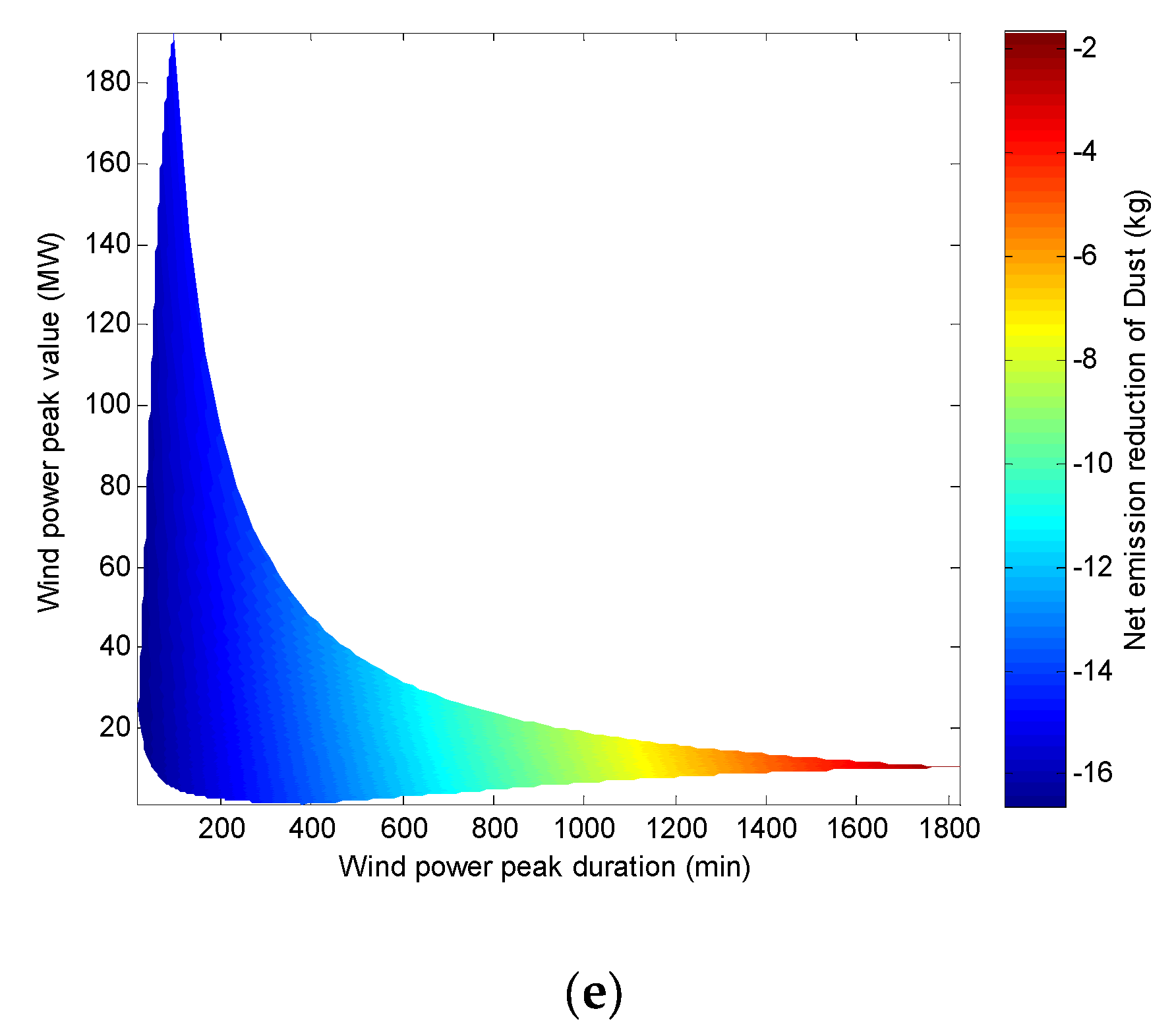
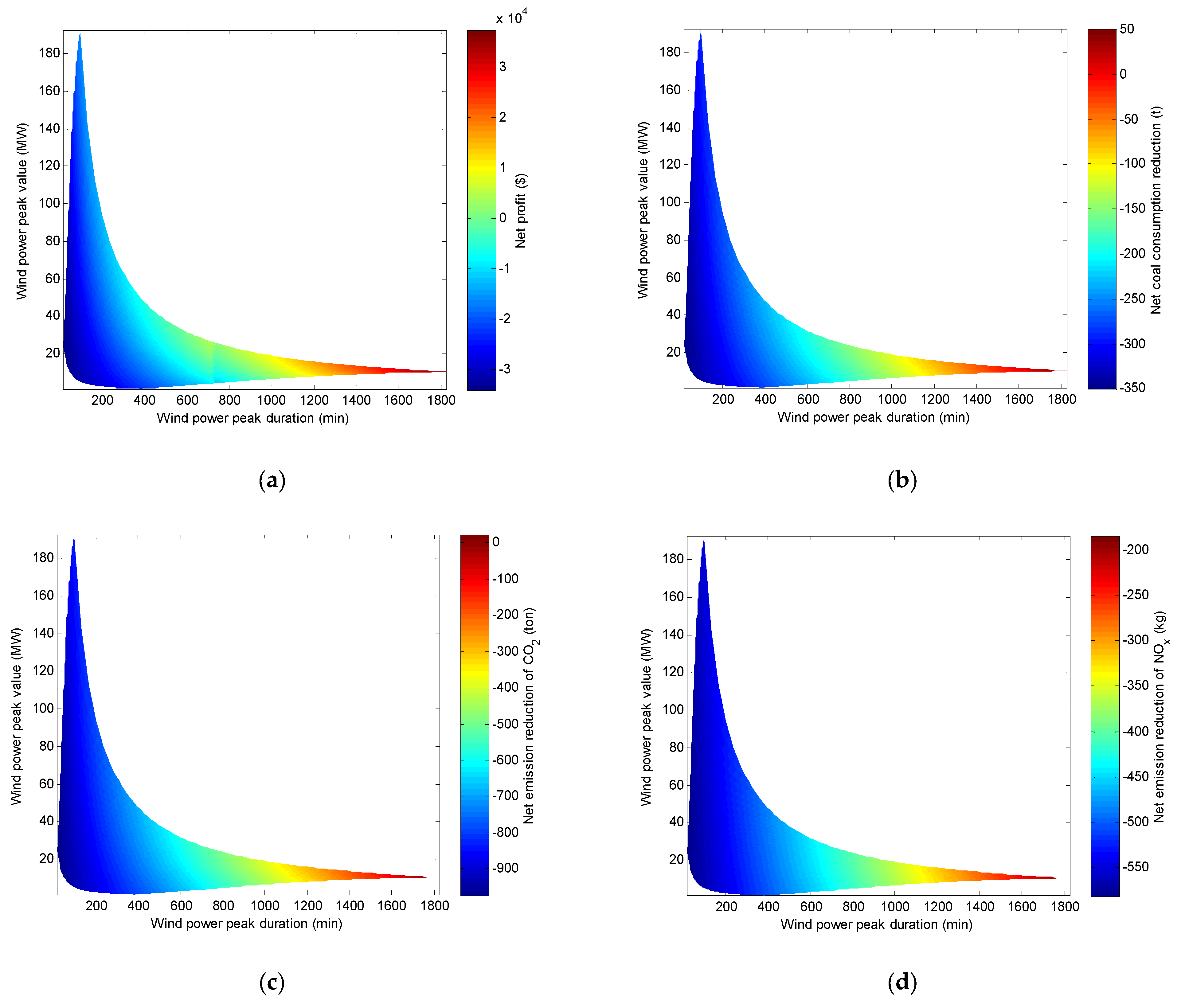
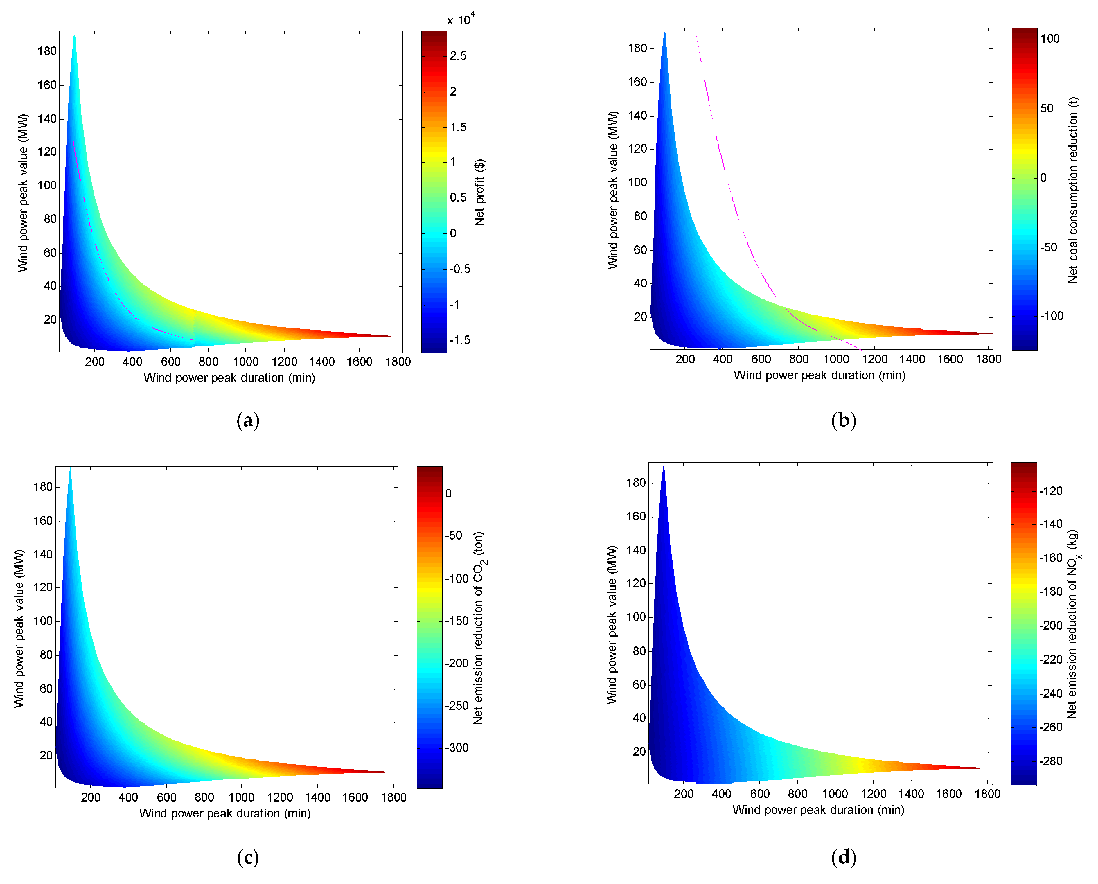
4.1. Wind Power Peaks above 540 MW

(1)

No wind energy curtailment mode 1 (300 MW unit start–stop peaking regulation)

Compared with the wind energy curtailment strategy, the relationships between the net profit/net reduction of the wind–coal combined base load power generation system and the wind power peak height H and peak width T are shown in Figure 6.

In Figure 6a, the dotted line is the wind energy curtailment boundary, in which the net benefit is the decision indicator. The boundary line is generated by fitting some (T, H) points with approximately zero net profit, and wind energy of wind power peak should be curtailed in the lower left of the boundary line. Four representative points on the boundary line were selected, and the corresponding wind power peak duration, peak height, power generation, and the power generation costs with different strategies are shown in

Table 3. Wind energy curtailment boundary with net income as the decision target.

Boundary Points	Duration (min)	Height (MW)	Power Quantity (MW·h)	Cost for Wind Energy Curtailment (×105 $)	Cost for Mode 1 (×105 $)
1	563	2.9	17.58	1.7934	1.7933
2	440	11.16	50.63	1.4230	1.4227
3	331	24.42	79.63	1.0937	1.0933
4	194	65.18	115.53	0.6815	0.6811

.

The dotted line in Figure 6b is the wind energy curtailment boundary line with the net coal saving amount as the decision index. The boundary line is generated by the fitting of some (T, H) points corresponding to the net coal saving amount at approximately zero. The wind power peaks (T, H) corresponding to the points in the lower left area of the corresponding boundary line should be abandoned. Four representative points on the boundary line were selected, and the corresponding wind power peak duration, peak height, power generation, and the system power generation coal consumption corresponding to two different strategies are shown in

Table 4. Wind energy curtailment boundary with net coal saving as the decision target.

Boundary Points	Duration (min)	Height (MW)	Power Generation Quantity (MW·h)	Coal Consumption for Wind Power Curtailment Mode (×103 t)	Coal Consumption for Mode 1 (×103 t)
1	948	6.24	60.14	1.7978	1.7969
2	899	10.25	89.24	1.7052	1.7046
3	856	14.80	115.53	1.6231	1.6228
4	823	19.44	136.01	1.5595	1.5594

.

The dotted line in Figure 6c is the wind energy curtailment boundary line with the CO₂ net emission reduction as the decision indicator. The boundary line is generated by the fitting of some (T, H) points when the CO₂ net emission reduction is approximately zero. The wind power peaks (T, H) corresponding to the points in the lower left area of the boundary line should be abandoned. Four representative points on the boundary line were selected, and the corresponding wind power peak duration, peak height, power generation quantity, system CO₂ emissions corresponding to two different strategies are shown in

Table 5. Wind energy curtailment boundary with CO₂ net emission reduction as the decision target.

Boundary Points	Duration (min)	Height (MW)	Power Generation Quantity (MW·h)	Emitted CO2 for Wind Energy Curtailment (×103 t)	Emitted CO2 for Mode 1 (×103 t)
1	1141	7.88	87.34	5.0557	5.0573
2	1075	10.48	107.31	4.8731	4.8724
3	1063	14.02	129.92	4.7111	4.7120
4	1022	18.66	149.99	4.5301	4.5290

.

The dotted line in Figure 6d is the wind energy curtailment boundary line with the NO_x net emission reduction as the decision indicator. The boundary line is generated by the fitting of some (T, H) points when the NO_x net emission reduction is approximately zero. The wind power peaks (T, H) corresponding to the points in the lower left area of the boundary line should be abandoned. Four representative points on the boundary line were selected, the corresponding wind power peak duration, peak height, power quantity generation, and the system NO_x emissions corresponding to two different strategies are shown in

Table 6. Wind energy curtailment boundary with NO_x net emission reduction as the decision target.

Boundary Points	Duration (min)	Height (MW)	Power Quantity (MW·h)	Emitted NOx for Wind Energy Curtailment Mode (kg)	Emitted NOx for Mode 1 (kg)
1	916	6.24	58.21	750.3547	750.3201
2	922	10.00	89.24	754.6157	755.2209
3	929	16.00	136.01	761.4154	762.4493
4	931	19.42	146.01	761.8848	762.9060

.

In Figure 6e, the wind energy curtailment boundary line is beyond the simulation range of this example and therefore fails to fit.

Overall, from the perspective of net profit, net coal savings, net CO₂ emission reduction and net NO_x reduction, the wind energy curtailment boundary line (dashed line in the figures) is closer to the lower left, that is, only the wind power peak with small T and H is suitable for the wind energy curtailment strategy. This is because the 300 MW unit has small start-up cost, coal consumption, CO₂ emissions and NO_x emissions in the no wind energy curtailment mode 1. From the perspective of dust emission reduction, the wind energy curtailment boundary line is at the upper right, that is to say, the wind energy curtailment strategy is required in the ranges with larger T and H.

(2)

No wind energy curtailment mode 2 (600 MW unit start and stop peaking regulation)

Compared with wind energy curtailment mode, the relationship between net profit/net reduction and wind power peak height H and peak width T is shown in Figure 7.

It can be seen in Figure 7 that from the perspective of net profit, net coal saving, net CO₂ reduction and net NO_x reduction, the wind energy curtailment boundary line is offset to the upper right side compared to no wind energy curtailment mode 1, that is, the abandoned wind range (T and H) has expanded. This is because the 600 MW unit has larger start-up cost, coal consumption, CO₂ emissions and NO_x emissions in the no wind energy curtailment mode 2. From the perspective of dust emission reduction, the wind energy curtailment boundary line moves to the lower left side compared with the no wind energy curtailment mode 1. That is to say, it is suitable to adopt the wind energy curtailment strategy in the smaller T and H range, which is mainly initiated by the different dust emission characteristics of the two units.

In general, on the decision-making line of the wind power 540 MW, the decision-making rules of net profit, net coal savings, net CO₂ reduction and net NO_x reduction are basically the same. The decision made using net dust emission reduction as the decision-making goal presents the opposite law. However, since the units use advanced dust precipitation technology and the overall dust emission is small, the dust emission can be ignored when making an operation decision.

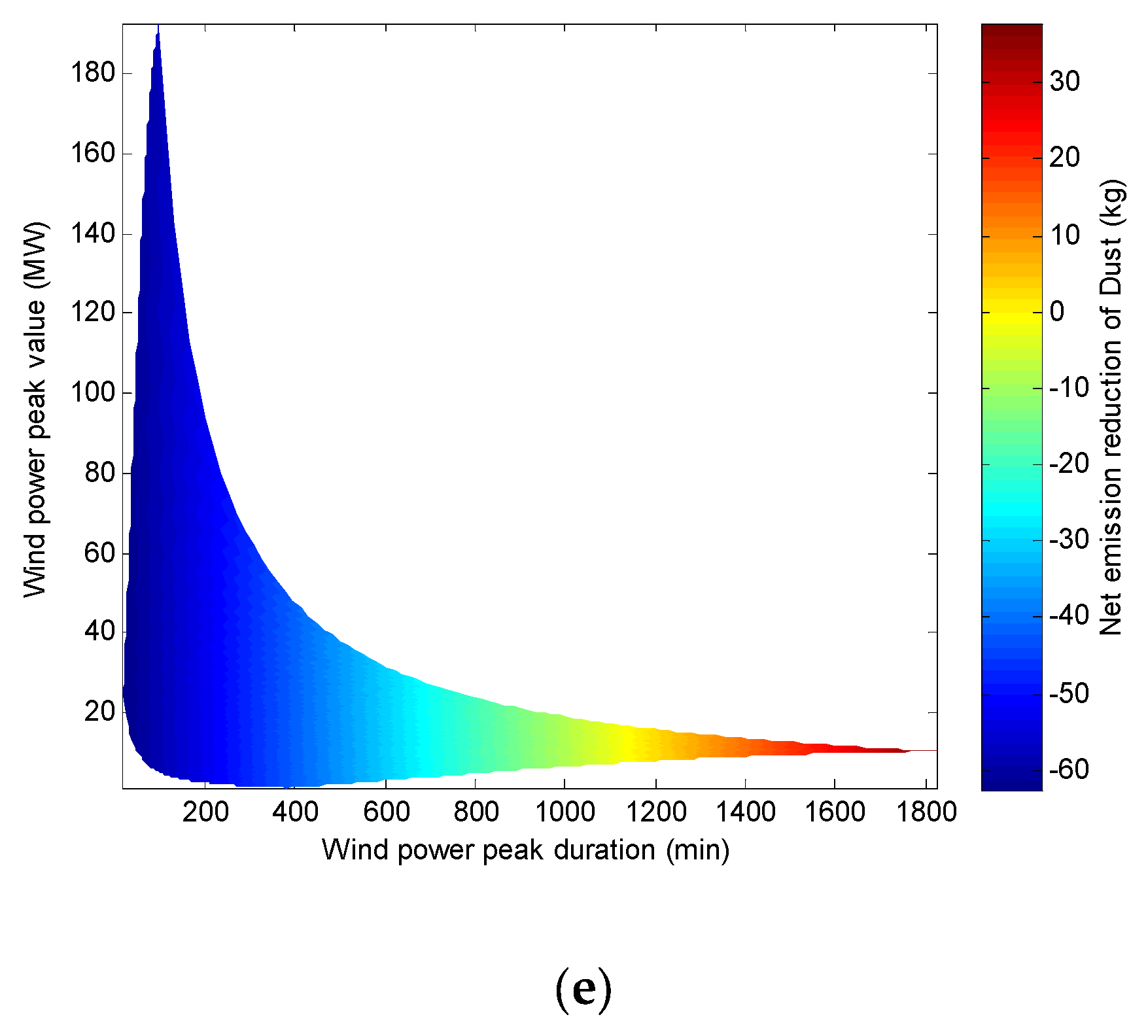
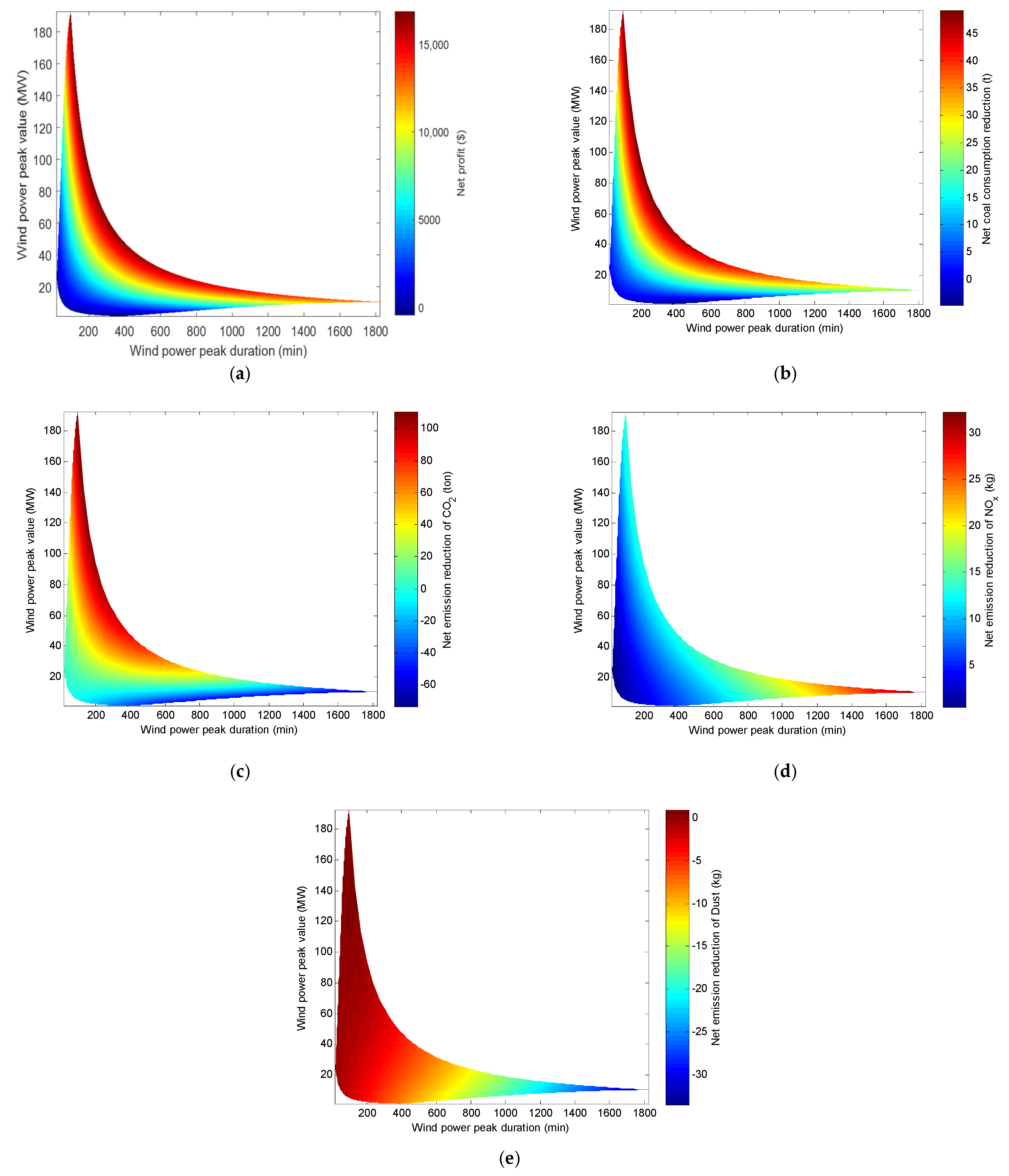
4.2. Wind Power Peaks above 240 MW

(1)

No wind energy curtailment (300 MW unit operates at 33% load, 600 MW unit operates for peak shaving)

Compared to the wind energy curtailment strategy (300 MW and 600 MW unit work together with a load 600 MW), the relationship between net profit/net reduction and wind power peak height H and peak width T is shown in Figure 8.

It can be seen that from the perspective of net profit, net coal saving, net CO₂ reduction and net NO_x reduction, the wind energy curtailment boundary line is closer to the lower left, that is, the wind energy curtailment strategy should be adopted only when wind power peak duration T and peak height H are very small. This is because the 300 MW unit has a fixed load, and the 600 MW unit has a variable peak load peaking in the no wind energy curtailment mode 1. There is no additional coal consumption, CO₂ emissions and NO_x emissions caused by the start-up and shutdown of the unit. From the perspective of dust emission reduction, the wind energy curtailment boundary line is close to the left side line, that is to say, when the peak width T is larger than a small value, the wind energy curtailment strategy should be adopted.

(2)

No wind energy curtailment (300 MW unit undergoes shutdown, 600 MW unit operates for peak shaving)

Compared to the wind energy curtailment strategy, the relationship between net profit/net emission reduction and wind power peak height H and peak width T is shown in Figure 9.

It can be seen that due to the use of 300 MW units to start and stop peaking, from the perspective of net profit, net coal savings, net CO₂ reduction and net emission reduction NO_x, the wind energy curtailment boundary line moves to the upper right, that is to say, the wind energy curtailment range (T and H) has expanded, especially for the net reduction of CO₂ and NO_x. From the perspective of dust emission reduction, the wind energy curtailment boundary line is closer to the left side line, and the wind energy curtailment range is further expanded.

That is to say, on the decision line of 240 MW wind power, the decision rules of net profit, net coal saving, net emission reduction CO₂, net emission reduction NO_x and net dust emission reduction decision targets are basically the same. The wind energy curtailment range (T, H) of mode 2 is expanded compared with mode 1.

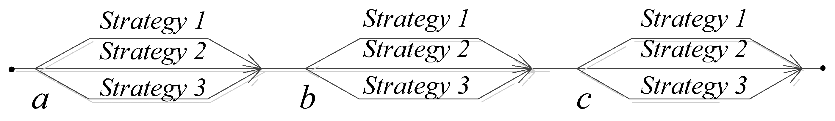
4.3. Operational Strategy Decision of Weekly Scale Wind–Coal Power Generation System

The operation decision of the weekly scale coal-fired power generation system refers to the process of rolling decision-making on a weekly basis. The decision-making target can be the cost of the whole week, the consumption of standard coal, the emission of CO₂, and the discharge of pollutants. Taking a wind–coal combined power generation system in an area as an example, the electric load is 840 MW, and the wind power output is the theoretical wind power of the wind power system in the region. Taking a representative week as an example, the wind power curve and the complementary coal power curve are shown in Figure 5.

It can be seen from Figure 5 that there are five points a, b, c, d, and e that need to be determined by the unit during the week. The time T and height H of the wind power peak curve corresponding to the two points d and e are small, and the utilization is small. The respective T and H are compared with those of Figure 8 and Figure 9. They are suitable for adopting the abandonment strategy and thus are no longer used as decision points in the subsequent decision-making process. A week’s operational decision can be represented by the decision tree in the figure below (Figure 10).

Strategy 1—wind energy curtailment; strategy 2—300 MW (100 MW) + 600 MW (peak shaving); strategy 3—600 MW (peak shaving)

The cost, standard coal consumption, CO₂ emissions, NO_x emissions, and dust emissions can be calculated under different operational strategies for three decision points a, b, and c, respectively, and obtain a net increase of strategy 2 and strategy 3 compared with strategy 1. Revenue, net coal consumption and net emission reduction are shown in

Table 7. The net revenue/coal saving and emission reduction corresponding to the wind energy curtailment strategy.

Decision Strategy		Net Revenue (×104 $)	Standard Coal (t)	CO2 (t)	NOx (kg)	Dust (kg)
Decision point a	Strategy 2	9.534	252.4	574.4	95.1	3.6
	Strategy 3	9.265	175.1	283.1	−155.7	−18.5
Decision point b	Strategy 2	112.207	2967.2	6967.0	268.7	57.9
	Strategy 3	120.92	3427.7	7929.0	566.9	58.9
Decision point c	Strategy 2	52.074	1436.3	3358.7	207.9	27.1
	Strategy 3	54.246	1505.1	3398.5	217.2	13.1

.

It can be seen that the net revenue, net coal saving and net emission reduction of strategy 2 at decision point a are greater than strategy 3, so strategy 2 should be used; at decision point b, the net revenue, net coal saving and net emission reduction of strategy 3 are greater than strategy 2, so strategy 3 should be used; strategy 3 is better than strategy 2 except for dust net reduction at decision point c, and strategy 3 should also be used for comprehensive consideration.

In order to verify the decision results above, the standard coal consumption, CO₂ emissions, NO_x emissions, and dust emissions corresponding to the 27 combined operation strategies for the week were calculated, as shown in

Table 8. Weekly coal consumption and atmospheric emissions from the combined decision.

Strategies	a	b	c	Coal Consumption (t)	CO2 (t)	NOx (kg)	Dust (kg)
1	a1	b1	c1	16,226.2	38,033.0	4417.8	591.0
2	a1	b1	c2	14,789.9	34,674.3	4209.9	563.7
3	a1	b1	c3	14,721.1	34,634.5	4200.6	577.7
4	a1	b2	c1	13,259.0	31,066.0	4149.1	533.1
5	a1	b2	c2	11,822.7	27,707.3	3941.2	505.8
6	a1	b2	c3	11,753.9	27,667.5	3931.9	519.8
7	a1	b3	c1	12,798.5	30,104.0	3850.9	532.2
8	a1	b3	c2	11,362.2	26,745.3	3643.0	504.8
9	a1	b3	c3	11,293.4	26,705.5	3633.7	518.8
10	a2	b1	c1	15,973.8	37,458.6	4322.7	587.4
11	a2	b1	c2	14,537.5	34,099.9	4114.8	560.1
12	a2	b1	c3	14,468.7	34,060.1	4105.5	574.1
13	a2	b2	c1	13,006.6	30,491.6	4054.0	529.5
14	a2	b2	c2	11,570.3	27,132.9	3846.1	502.2
15	a2	b2	c3	11,501.5	27,093.1	3836.8	516.2
16	a2	b3	c1	12,546.1	29,529.6	3755.8	528.5
17	a2	b3	c2	11,109.8	26,170.9	3547.9	501.2
18	a2	b3	c3	11,041.0	26,131.1	3538.6	515.2
19	a3	b1	c1	16,051.1	37,749.9	4573.5	609.6
20	a3	b1	c2	14,614.8	34,391.2	4365.6	582.3
21	a3	b1	c3	14,546.0	34,351.4	4356.3	596.3
22	a3	b2	c1	13,083.9	30,782.9	4304.8	551.7
23	a3	b2	c2	11,647.6	27,424.2	4096.9	524.4
24	a3	b2	c3	11,578.8	27,384.4	4087.6	538.4
25	a3	b3	c1	12,623.4	29,820.9	4006.6	550.7
26	a3	b3	c2	11,187.1	26,462.2	3798.7	523.4
27	a3	b3	c3	11,118.3	26,422.4	3789.4	537.4

. It can be seen that the optimal combination is the 18th combination (a2, b3, c3), with smallest weekly coal consumption, CO₂ emission and NO_x emission of 11041.0 t, 26131.1 t and 3538.6 kg, respectively. Additionally, wind energy curtailment strategy is not always the worst operation strategy. For example, the emissions of NO_x and dust in the 19th combination are greater than the wind energy curtailment strategy (1st combination).

5. Conclusions

For wind–coal combined power generation systems, as the wind power penetration rate increases, the coal-fired power units in the network need to operate more flexibly (including frequent deep peak shaving, and frequent start-up and shutdown). Flexible operation of coal-fired units has different energy consumption and emission characteristics, so the impact of flexible operations should be considered when making optimal unit decisions (including wind curtailment). According to the output profile of wind power, a wind power peak simulation model based on Gaussian distribution is established to simulate peaks with different shapes (T, H). For the wind-fired combined base load (840 MW) power generation system, the decision criteria of maximum wind power output at 540 MW and 240 MW were given, respectively, and the wind energy curtailment boundary line of different decision targets was determined through simulation calculation.

The simulation results show that when the wind power is above 540 MW, the wind energy curtailment range of mode 2 is enlarged compared to mode 1 from the aspect of the net profit, the net coal saving, the net CO₂ reduction and the net NO_x reduction. The decision-making rules of net profit, net coal saving, net CO₂ reduction and net emission reduction NO_x are basically the same. The decision to use the net emission reduction of dust as the decision-making goal is opposite, because the dust emission is relatively small and can be ignored. When the wind power is above 240 MW, the wind energy curtailment range (T and H) of mode 2 is larger than mode 1 from the aspect of net profit, net coal saving, net CO₂ emission reduction and net NO_x emission reduction, especially for net CO₂ reduction and net NO_x reduction, indicating that shutdown and then start-up coal units for accommodating wind power is not an efficient operation strategy. At the same time, the decision-making rules for different decision objectives, such as net profit, net coal saving, net emission reduction CO₂, net emission reduction NO_x and net emission reduction dust are basically the same. The decision-making analysis of the wind–coal combined base load 840 MW power generation system with actual wind power was carried out. Among all combinations, the 18th decision-making combination (a2, b3, c3) was optimal, with smallest weekly coal consumption, CO₂ emission and NO_x emission of 11,041.0 t, 26,131.1 t and 3538.6 kg, respectively; the 1st decision combination (a1, b1, c1) was the worst, with largest weekly coal consumption and CO₂ emission of 16,226.2 t, 38,033.0 t and second largest weekly NO_x emission of 4417.8 kg. Compared with 1st combination, the weekly coal consumption and CO₂ emission of 18th combination can be reduced by 32.0%, and the weekly NO_x emission can be reduced by 19.9%.

Our study can be applied in the operation decision-making of real wind–coal dominated generation systems. On the base of load forecasting and wind power forecasting, the unit commitment and wind curtailment (if necessary) decision can be made according to predicted wind power profiles (T and H) and wind curtailment ranges. Our study has shown that in the decision-making of the unit input in the power system is important not simply to reduce wind curtailment rate, but also to take factors such as energy consumption, CO₂ emissions and air pollutant emissions into consideration. The study also revealed the importance of unit commitment/dispatch research for a real wind–coal combined power system. This paper highlights two points below:

(1)

According to the peak characteristics of the power curve of the wind farm, a simulation model of the peak of the wind power curve was established based on the Gaussian distribution, and the simulation of the peaks of different shapes was achieved by changing the parameter σ of the Gaussian distribution function;

(2)

Based on the research of a base load wind–coal combined power generation system with high-proportion wind power, a decision-making model of the unit operation strategy was established based on economic and environmental criteria. The decision objective function considered the costs and pollutant emissions increase caused by deep peak regulation and fast start-up and shutdown.

Future studies should focus on the optimal operation strategy of wind power and coal power under the fluctuating load in actual operating conditions, and the coordinated optimal operation strategy of the entire power system equipped with the energy storage power module.

References

1. NDRC; SERC. Notification of The Renewable Energy Tariff Subsidy and Quota Trading Scheme. 2011. Available online: http://www.ndrc.gov.cn/fzgggz/jggl/zcfg/201102/t20110215_748295.html (accessed on 5 March 2020).
2. NDRC; NEA. The 13th FYP Power Development Planning. 2016. Available online: https://zfxxgk.ndrc.gov.cn/web/fileread.jsp?id=240 (accessed on 5 March 2020).
3. NEA; NDRC. Guidance on The Implementation of the 13th Five-Year Plan for Renewable Energy Development. 2017. Available online: http://zfxxgk.nea.gov.cn/auto87/201707/t20170728_2835.htm (accessed on 5 March 2020).
4. Yuan, J.H. Wind energy in China: Estimating the potential. Nat. Energy 2016, 1, 16095. [Google Scholar] [CrossRef]
5. Yuan, J.H.; Xu, Y. Peak energy consumption and CO2 emissions in China. Energy Policy 2014, 68, 508–523. [Google Scholar] [CrossRef]
6. Yuan, J.H.; Xu, Y. China’s 2020 clean energy target: Consistency, pathways and policy implications. Energy Policy 2014, 65, 692–700. [Google Scholar] [CrossRef]
7. Yuan, J.; Lei, Q.; Xiong, M.; Guo, J.S.; Hu, Z. The prospective of coal power in China: Will it reach a plateau in the coming decade. Energy Policy 2016, 98, 495–504. [Google Scholar] [CrossRef]
8. Denny, E.; O’Malley, M. Wind generation, power system operation, and emissions reduction. IEEE Trans. Power Syst. 2006, 21, 341–347. [Google Scholar] [CrossRef]
9. Katzenstein, W.; Jay, A. Air emissions due to wind and solar power. Environ. Sci. Technol. 2009, 43, 253–258. [Google Scholar] [CrossRef] [Green Version]
10. Valentino, L.; Valenzuela, V.; Botterud, A. System-wide emissions implications of increased wind power penetration. Environ. Sci. Technol. 2012, 46, 4200–4206. [Google Scholar] [CrossRef]
11. Zhao, X.L.; Liu, S.W.; Yan, F.G.; Yuan, Z.Q.; Liu, Z.W. Energy conservation, environmental and economic value of the wind power priority dispatch in China. Renew. Energy 2017, 111, 666–675. [Google Scholar] [CrossRef]
12. Oates, D.L.; Jaramillo, P. Production cost and air emissions impacts of coal cycling in power systems with large-scale wind penetration. Environ. Res. Lett. 2013, 8, 024022–024028. [Google Scholar]
13. Lu, X.; McElroy, M.B.; Chen, X. Opportunity for offshore wind to reduce future demand for coal-fired power plants in China with consequent savings in emissions of CO2. Environ. Sci. Technol. 2014, 48, 14764–14771. [Google Scholar] [CrossRef] [Green Version]
14. Gonzalez-Salazara, M.A.; Kirsten, T.; Prchlik, L. Review of the operational flexibility and emissions of gas- and coal-fired power plants in a future with growing renewables. Renew. Sustain. Energy Rev. 2018, 82, 1497–1513. [Google Scholar] [CrossRef]
15. Yang, H.; Liang, R.; Yuan, Y.; Chen, B.; Xiang, S.; Liu, J.; Ackom, E. Distributionally robust optimal dispatch in the power system with high penetration of wind power based on net load fluctuation data. Appl. Energy 2022, 313, 118813–118828. [Google Scholar] [CrossRef]
16. Li, Y.; Wang, J.; Han, Y.; Zhao, Q.; Fang, X.; Cao, Z. Robust and opportunistic scheduling of district integrated natural gas and power system with high wind power penetration considering demand flexibility and compressed air energy storage. J. Clean. Prod. 2020, 256, 120456–120474. [Google Scholar] [CrossRef]
17. NREL. The Western Wind and Solar Integration Study 2; NREL/TP-5500-55888; National Renewable Energy Laboratory: Golden, CO, USA, 2013. [Google Scholar]
18. Frade, P.M.; Pereira, J.P.; Santana, J.J.E.; Catalão, J.P.S. Wind balancing costs in a power system with high wind penetration—Evidence from Portugal. Energy Policy 2019, 132, 702–713. [Google Scholar] [CrossRef]
19. Dong, Y.; Jiang, X.; Liang, Z.; Yuan, J. Coal power flexibility, energy efficiency and pollutant emissions implications in China: A plant-level analysis based on case units. Resour. Conserv. Recycl. 2018, 134, 184–195. [Google Scholar] [CrossRef]
20. Dong, Y.; Jiang, X.; Ren, M.; Yuan, J. Environmental implications of China’s wind-coal combined power generation system. Resour. Conserv. Recycl. 2019, 142, 24–33. [Google Scholar] [CrossRef]
21. Kubik, M.L.; Coker, P.J.; Barlow, J.F. Increasing thermal plant flexibility in a high renewables power system. Appl. Energy 2015, 154, 102–111. [Google Scholar] [CrossRef] [Green Version]
22. Hübel, M.; Meinke, S.; Andrén, M.T.; Wedding, C.; Nocke, J.; Gierow, C.; Funkquist, J. Modelling and simulation of a coal-fired power plant for start-up optimization. Appl. Energy 2017, 208, 319–331. [Google Scholar] [CrossRef]
23. Wang, W.; Liu, J.; Zeng, D.; Niu, Y.; Cui, C. Modeling for condensate throttling and its application on the flexible load control of power plants. Appl. Therm. Eng. 2016, 95, 303–310. [Google Scholar] [CrossRef]
24. Wang, W.; Li, L.; Long, D.; Liu, J.; Zeng, D.; Cui, C. Improved boiler-turbine coordinated control of 1000 MW power units by introducing condensate throttling. J. Process Control. 2017, 50, 11–18. [Google Scholar] [CrossRef]
25. Zhou, Y.; Wang, D. An improved coordinated control technology for coal-fired boiler-turbine plant based on flexible steam extraction system. Appl. Therm. Eng. 2017, 125, 1047–1060. [Google Scholar] [CrossRef]
26. Garbrecht, O.; Bieber, M.; Kneer, R. Increasing fossil power plant flexibility by integrating molten-salt thermal storage. Energy 2017, 118, 876–883. [Google Scholar] [CrossRef]
27. Richter, M.; Oeljeklaus, G.; Görner, K. Improving the load flexibility of coal-fired power plants by theintegration of a thermal energy storage. Appl. Energy 2019, 236, 607–621. [Google Scholar] [CrossRef]
28. Wolfersdorf, C.; Boblenz, K.; Pardemann, R.; Meyer, B. Syngas-based annex concepts for chemical energy storage and improving flexibility of pulverized coal combustion power plants. Appl. Energy 2015, 156, 618–627. [Google Scholar] [CrossRef]
29. Mahdia, F.P.; Vasanta, P.; Kallimanib, V. A holistic review on optimization strategies for combined economic emission dispatch problem. Renew. Sustain. Energy Rev. 2018, 81, 3006–3020. [Google Scholar] [CrossRef]
30. Zhao, X.L.; Wu, L.L.; Zhang, S.F. Joint environmental and economic power dispatch considering wind power integration: Empirical analysis from Liaoning Province of China. Renew. Energy 2013, 52, 260–265. [Google Scholar] [CrossRef]
31. El-Keib, A.; Ding, H. Environmentally constrained economic dispatch using linear programming. Electr. Power Syst. Res. 1994, 29, 155–159. [Google Scholar] [CrossRef]
32. Chen, J.F.; Chen, S.D. Multi-objective power dispatch with line flow constraints using the fast Newton-raphson method. IEEE Trans. Energy Convers. 1997, 12, 86–93. [Google Scholar] [CrossRef]
33. Wang, K.P.; Yuryevich, J. Evolutionary-programming-based algorithm for environmentally-constrained economic dispatch. IEEE Trans. Power Syst. 1998, 13, 301–306. [Google Scholar] [CrossRef]
34. Das, D.B.; Patvardhan, C. New multi-objective stochastic search technique for economic load dispatch. IEEE Proc. Gener. Transm. Distrib. 1998, 145, 747–752. [Google Scholar] [CrossRef]
35. Song, Y.H.; Wang, G.S.; Wang, P.Y.; Johns, A.T. Environmental/economic dispatch using fuzzy logic controlled genetic algorithms. IEEE Proc. Gener. Transm. Distrib. 1997, 144, 377–382. [Google Scholar] [CrossRef]
36. Kumar AI, S.; Dhanushkodi, K.; Kumar, J.J.; Paul, C.K.C. Particle swarm optimization solution to emission and economic dispatch problem. In Proceedings of the TENCON 2003 Conference on Convergent Technologies for the Asia-Pacific Region, Bangalore, India, 15–17 October 2003; pp. 435–439. [Google Scholar]
37. Basu, M. A simulated annealing-based goal-attainment method for economic emission load dispatch of fixed head hydrothermal power systems. Int. J. Electr. Power Energy Syst. 2005, 27, 147–153. [Google Scholar] [CrossRef]
38. Apostolopoulos, T.; Vlachos, A. Application of the firefly algorithm for solving the economic emissions load dispatch problem. Int. J. Comb. 2011, 2011, 523806. [Google Scholar] [CrossRef] [Green Version]
39. Dixit, G.P.; Dubey, H.M.; Pandit, M.; Panigrahi, B.K. Artificial bee colony optimization for combined economic load and emission dispatch. In Proceedings of the Sustainable Energy and Intelligent Systems, International Conference on: IET, Chennai, India, 20–22 July 2011; pp. 340–345. [Google Scholar]
40. Ramesh, B.; Chandra Jagan Mohan, V.; Veera Reddy, V.C. Application of bat algorithm for combined economic load and emission dispatch. J. Electr. Eng. 2013, 13, 214–219. [Google Scholar]
41. Roy, P.K.; Bhui, S. A multi-objective hybrid evolutionary algorithm for dynamic economic emission load dispatch. Int. Trans. Electr. Energy Syst. 2016, 26, 49–78. [Google Scholar] [CrossRef]
42. Zhang, H.; Yue, D.; Xie, X.; Hu, S.; Weng, S. Multi-elite guide hybrid differential evolution with simulated annealing technique for dynamic economic emission dispatch. Appl. Soft Comput. 2015, 34, 312–323. [Google Scholar] [CrossRef]
43. Younes, M.; Khodja, F.; Kherfane, R.L. Multi-objective economic emission dispatch solution using hybrid FFA (firefly algorithm) and considering wind power penetration. Energy 2014, 67, 595–606. [Google Scholar] [CrossRef]
44. Sayah, S.; Hamouda, A.; Bekrar, A. Efficient hybrid optimization approach for emission constrained economic dispatch with nonsmooth cost curves. Int. J. Electr. Power Energy Syst. 2014, 56, 127–139. [Google Scholar] [CrossRef]
45. Hooshmand, R.A.; Parastegari, M.; Morshed, M.J. Emission, reserve and economic load dispatch problem with non-smooth and non-convex cost functions using the hybrid bacterial foraging-Nelder-Mead algorithm. Appl. Energy 2012, 89, 443–453. [Google Scholar] [CrossRef]
46. Roselyn, J.P.; Devaraj, D.; Dash, S.S. Economic Emission OPF Using Hybrid GA-Particle Swarm Optimization. In International Conference on Swarm, Evolutionary, and Memetic Computing; Springer: Berlin/Heidelberg, Germany, 2011; pp. 167–175. [Google Scholar]
47. Hota, P.; Barisal, A.; Chakrabarti, R. Economic emission load dispatch through fuzzy based bacterial foraging algorithm. Int. J. Electr. Power Energy Syst. 2010, 32, 794–803. [Google Scholar] [CrossRef]
48. Ramadan, A.; Ebeed, M.; Kamel, S.; Agwa, A.M.; Tostado-Véliz, M. The Probabilistic Optimal Integration of Renewable Distributed Generators Considering the Time-Varying Load Based on an Artificial Gorilla Troops Optimizer. Energies 2022, 15, 1302. [Google Scholar] [CrossRef]
49. Kuo, C.C. Wind energy dispatch considering environmental and economic factors. Renew. Energy 2010, 35, 2217–2227. [Google Scholar] [CrossRef]
50. Bishop, C. Pattern Recognition and Machine Learning; Springer: Berlin/Heidelberg, Germany, 2007. [Google Scholar]
51. NB/T 31110-2017; Technical Rule for Active Power Regulation and Control of Wind Farm. National Energy Administration: Beijing, China, 2017.
52. Soliman, S.A.H.; Mantawy, A.A.H. Modern Optimization Techniques with Applications in Electric Power Systems; Springer: Berlin/Heidelberg, Germany, 2018. [Google Scholar]
Figure 1. Wind power output curve for one month.
Energies 15 08004 g001
Figure 2. Wind power output curve for one week.
Energies 15 08004 g002
Figure 3. Gaussian distribution function.
Energies 15 08004 g003
Figure 4. Simulated wind power peak curve using Gaussian distribution.
Energies 15 08004 g004
Figure 5. Wind power curve and complementary coal power curve.
Energies 15 08004 g005
Figure 6. Net profit and net emission reduction of the wind–coal combined power generation system of strategy (2) against wind energy curtailment for wind power peaks above 540 MW. (a) Net profit; (b) Net coal consumption reduction; (c) Net emission reduction of CO2; (d) Net emission reduction of NOx; (e) Net emission reduction of dust.
Energies 15 08004 g006aEnergies 15 08004 g006b
Figure 7. Net profit and net emission reduction of the wind–coal combined power generation system of strategy (3) against wind energy curtailment strategy for wind power peaks above 540 MW. (a) Net profit; (b) Net coal consumption reduction; (c) Net emission reduction of CO2; (d) Net emission reduction of NOx; (e) Net emission reduction of dust.
Energies 15 08004 g007aEnergies 15 08004 g007b
Figure 8. Net profit and net emission reduction of the wind–coal combined power generation system of strategy (2) against wind energy curtailment for wind power peaks above 240 MW. (a) Net profit; (b) Net coal consumption reduction; (c) Net emission reduction of CO2; (d) Net emission reduction of NOx; (e) Net emission reduction of dust.
Energies 15 08004 g008
Figure 9. Net profit and net emission reduction of the wind–coal combined power generation system of strategy (3) against wind energy curtailment for wind power peaks above 240 MW. (a) Net profit; (b) Net coal consumption reduction; (c) Net emission reduction of CO2; (d) Net emission reduction of NOx; (e) Net emission reduction of dust.
Energies 15 08004 g009aEnergies 15 08004 g009b
Figure 10. Decision tree.
Energies 15 08004 g010