Abstract
Multi-energy virtual power plants (MEVPPs) effectively realize multi-energy coupling. Low-carbon transformation of coal-fired units at the source side and consideration of demand response resources at the load side are important ways to achieve carbon peak and carbon neutralization. Based on this, this paper proposes a low-carbon economic dispatch model for the MEVPP system considering source-load coordination with comprehensive demand response. Combined with the characteristics of organic Rankine cycle (ORC) waste heat power generation and comprehensive demand response energy to increase the flexibility on both sides of the source and load, the problem of insufficient carbon capture during the peak load period in the process of low-carbon transformation of thermal power units has been improved. First, the ORC waste heat recovery device is introduced into the MEVPP system to decouple the cogeneration unit’s “heat-based electricity” constraint, which improves the flexibility of the unit’s power output. Secondly, we consider the synergistic effect of the comprehensive demand response and ORC waste heat recovery device and analyze the source-load coordination low-carbon dispatch mechanism. Finally, an example simulation is carried out in a typical system. The simulation example shows that this method effectively improves the carbon capture level of carbon capture power plants, takes into account the economy and low carbon of the system, and can provide a reference for the low-carbon economic dispatch of the MEVPP system.
1. Introduction
To cope with the new landscape and tasks brought about by carbon peaking and carbon neutrality goals, various countries have prioritized the promotion of low-carbon energy transformation [1]. Virtual power plants (VPPs) can integrate renewable energy, conventional units, and loads into an organic whole and have them show the characteristics of power plants through coordinated dispatching [2,3]. The development of a multi-energy virtual power plant system (MEVPP) and carbon capture and storage technology (CCS) provides a key means for realizing the low carbonization of the “source” side of the power system [4,5].
MEVPP has the advantages of multi-energy coupling and complementation, reducing energy costs and carbon emissions, and research on its low-carbon optimization operation has now become a topic of interest. Yang Q. et al. [6] have developed a virtual power plant management mode based on the blockchain to encourage users to use renewable energy, energy storage, flexible load, and other resources in the virtual power plant. Rahimi M. et al. [7] model the stochastic scheduling problem of virtual power plants to meet both thermal and electrical loads, considering network security constraints and uncertainties on both the supply and demand sides. Sikorski T. et al. [8] analyze the technical and economic possibilities of integrating various energy sources and energy storage into the operation of virtual power plants and evaluate the economic efficiency of the VPP model. Ghasemi Olanlari F. et al. [9] proposed a multi-energy virtual power plant (MEVPP) day-ahead scheduling optimization model, including electricity, heat and natural gas, and simultaneously participate in day-ahead energy, natural gas, heat markets and power spinning reserve markets. Alabi T M. et al. [10] proposed a new virtual power plant (VPP) day-ahead dispatch model that enables joint optimization of multi-energy systems and the multi-flexibility potential of electric vehicles. However, most MEVPP currently uses traditional coal-fired units or gas-fired units as the core power source, resulting in high levels of carbon emissions in the system.
Installing carbon capture equipment in coal-fired units can effectively reduce carbon emissions, but its energy consumption limits the carbon capture effect. Therefore, carbon capture and storage technology provide a new direction for MEVPP low-carbon operation [11,12,13]. After the thermal power is transformed into a carbon capture power plant, since the total output of the source-side Rankine cycle system remains unchanged, part of the electric energy is required for carbon capture, resulting in a reduction in the on-grid power of the carbon capture power plant during the peak load period [14].
At the same time, the electrical load and thermal load in MEVPP often have peak staggered characteristics, while the combined heat and power unit (CHP) is affected by the constraint of “determining electricity by heat”, which reduces the output during peak hours of electrical load, e.g., micro gas turbines (MT) [15,16]. Carbon capture devices often need to transfer part of the carbon capture energy consumption to supply loads. The problem of insufficient carbon capture levels during peak load periods is more prominent.
Given the above problems, the introduction of organic Rankine cycle (ORC) waste heat power generation on the source side can decouple the MT unit constraint of “determining electricity by heat” and increase the output of MT units during peak load periods [17,18]. In addition, due to the difficulty and high cost of supporting carbon capture technology for gas-fired units, the use of ORC waste heat power generation to decouple thermoelectricity has become a realistic choice. Xu B. et al. [19] proposed a model-free reinforcement learning method for online transient power optimization of organic Rankine cycle waste heat recovery (ORC-WHR) systems. They explained the advantages of the learning method in this application. Romanos P. et al. [20] proposed an energy management strategy for VPP that combines the organic Rankine cycle and thermal energy storage (TES) to optimize the charging of TES tanks during off-peak demand and to control the energy used to release energy during peak demand.
The wind power and photovoltaic output in the MEVPP system have strong randomness, which will affect the system’s stable operation. The commonly used uncertainty processing methods include stochastic optimization [21,22] and robust optimization [23,24,25]. Aguilar J. et al. [26] built a stochastic optimization layer on the model predictive control kernel and defined a stochastic model control scheme by combining chance constraints to deal with the uncertainty of VPP system operation. Jordehi A. R. [27] proposed a risk-averse two-stage stochastic model to guide the operation of VPPs with cogeneration properties, and studies the impact of different markets on VPP profits and risks. Considering the uncertainty of price and wind power output, Zhang Y. et al. [28] proposed a robust optimization model, which is used to formulate the optimal self-dispatching plan of VPP participation day-ahead energy. Yan Q. et al. [29] introduced the carbon trading mechanism into MEVPP and constructed a dynamic, robust optimization model considering the multiple uncertainty factors of source and load. However, robust optimization only makes the dispatching plan under the worst scenario, resulting in too conservative results. While stochastic optimization makes the results more practical by considering different scenarios for scheduling. One of the keys of stochastic optimization is scene generation and reduction, so it needs to be considered emphatically.
From the above analysis, it can be shown that: (1) At present, most of the related research on ORC waste heat power generation focuses on improving the thermoelectric coupling performance of the system, and very little research analyzes its contribution to low carbon levels. (2) Although the above literature introduced the coordination of MEVPP with carbon capture power plants, which improved the system carbon capture level to a certain extent, the carbon capture power plants could not maintain the highest carbon capture level. This problem is particularly serious during the peak load period, so its low-carbon characteristics must be further explored.
Based on this, the contributions of this paper are as follows:
- To solve the problem of insufficient carbon capture level in the low-carbon transformation process of thermal power plants, ORC waste heat power generation is introduced at the source side to expand the MT output range, and the demand response is considered at the load side. The carbon transaction cost is also added to the objective function to optimize the system operation cost further.
- The Latin hypercube sampling (LHS) method is used to build the scene to deal with the uncertainty of wind power output, photovoltaic output, and load, and the 0–1 scenario dimensionality reduction technology based on the Wasserstein metric is used to reduce the scene. Thus, the uncertainty of both sides of the source and load in the system can be effectively handled.
- The simulation is carried out in a typical MEVPP system. It also analyzes the effectiveness of the scheduling model proposed in this paper to solve the problem of insufficient carbon capture level of carbon capture power plants in the environment of the carbon trading market to reduce carbon emissions and system operating costs.
The rest of this paper is organized as follows: the structure of MEVPP is analyzed in Section 2. In Section 3, the operation model of the unit in MEVPP is introduced. Section 4 establishes the stochastic optimization dispatching model of the MEVPP system is established. The model is simulated from several angles in Section 5, and the main conclusions are presented in Section 6.
2. System Description
Based on conventional multi-energy VPP, this paper transforms coal-fired units into carbon capture units, as shown in Figure 1.
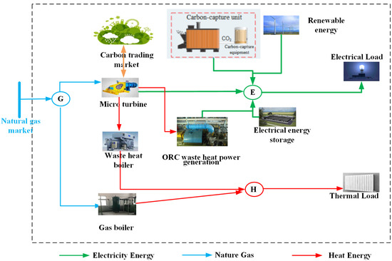
Figure 1.
MEVPP system structure.
It can be seen from Figure 1 that the electrical load in the MEVPP system is supplied by a carbon capture unit (CCU), renewable energy (including wind power (WT) and photovoltaic (PV)), microturbine (MT), electric energy storage (EES) and ORC waste heat power generation. The thermal load is supplied by a gas boiler (GB) and waste heat boiler (WB). Energy coupling equipment mainly includes MT, ORC waste heat power generation, and GB.
- Energy flow analysis
As an example for analysis, the natural gas flows into the gas boiler to output thermal power to supply the thermal load. Some natural gas flows into the MT to output electric power to produce electric energy, and the output heat energy is divided into two parts. One part flows to the waste heat recovery device for ORC waste heat power generation, and the output power is supplied to the electrical load, while the other part flows to the waste heat boiler to supply the thermal load. This also shows that the introduction of ORC waste heat power generation can realize MT’s flexible thermal and electrical response.
- 2.
- Operation principle of CCU
A carbon capture unit refers to a low-carbon power unit formed by the low-carbon transformation of traditional coal-fired units equipped with carbon capture equipment. The carbon capture device can capture and separate CO2 from the coal-fired process of coal-fired units and then transport it to oil and gas fields, oceans and other places for long-term storage or reuse so as to effectively reduce CO2 emissions [3]. The carbon capture level of carbon capture units is an important indicator of the low-carbon performance of carbon capture power plants. The insufficient carbon capture level of the carbon capture unit during peak load is one of the important factors restricting its development.
3. Main Equipment Models in MEVPP
3.1. Model of Energy Supply Equipment
3.1.1. Carbon Capture Unit (CCU)
A more flexible operation mode can be formed by introducing a flue gas bypass system and a solution reservoir into the carbon capture unit at the same time. This mode can not only transfer the carbon capture energy consumption to the low load at the peak of the load, alleviate the contradiction between the load demand and the carbon capture demand, but also increase the carbon capture energy consumption at the low load and reduce the net output of the carbon capture unit to absorb part of the abandoned wind power.
- Constraints of CCU output:
- 2.
- Constraints of CCU energy consumption:
- 3.
- Constraints of a solution storage tank in CCU
The CO2 extracted from the solution storage exists in the ethanolamine solution in the form of a compound. The relationship between the mass of CO2 and the volume of the ethanolamine solution needs to be considered. This paper refers to the processing method of Ref. [22] to convert the mass of CO2 that can be extracted from the solution storage into the form of solution volume, as shown in Equation (3a).
3.1.2. Micro Gas Turbines (MT)
A type of cogeneration equipment, the micro gas turbine is an important equipment in the MEVPP. That is to say, while the micro gas turbine generates electric energy, heat energy is used as a by-product to supply the cooling load and heating load of the whole system.
The mathematical model of gas consumption of MT and the residual heat in the exhaust gas is:
where, is the amount of gas consumed, and is the generating power of MT (MW). is the efficiency value, and is the low calorific value. is the heat loss coefficient of MT. is the residual heat in the flue gas discharged by the MT (MW).
The output power of the MT meets the operation constraints:
where, is the minimum output of MT (MW), and is the maximum output of MT (MW).
3.1.3. Waste Heat Boiler (WB)
The waste heat from the flue gas discharged by the MT is collected to supply the cold and heat load demand of the MEVPP system. The output heat of the WB is:
where, is the output heat of WB (MW), and is the input heat, that is, the waste heat collected (MW). and are the minimum and maximum heat output (MW), respectively.
3.1.4. Renewable Energy
The power restrictions of the renewable energy are listed as follows:
where, and are the output of wind power and PV (MW), respectively. and are the maximum output of wind power and PV (MW), respectively.
3.2. Model of Energy Conversion Equipment
3.2.1. ORC Waste Heat Power Generation
ORC waste heat power generation refers to the power generation technology that uses organics with low boiling point characteristics as working fluid, represented by R245fa. It can not only improve energy efficiency, but also upgrade low-quality waste heat resources to high-quality electric energy.
It can be seen from Figure 1 that the waste heat generated by the MT unit has two flow directions, namely, waste heat power generation through ORC and heat generation through WB. This effectively decouples the constraint of “determining electricity by heat”. The MT and ORC waste heat power generation model is constructed according to the energy flow relationship as follows:
where, is the residual heat transmitted to ORC (MW). is the power generation after ORC waste heat recovery (MW). is the power generation efficiency.
The output power of the ORC waste heat power generation unit meets the operation constraints:
where, and are the minimum and maximum output of ORC waste heat power generation (MW), respectively.
3.2.2. Gas Boiler (GB)
When the waste heat of MT is insufficient to supply the heat load demand of the cogeneration system, the gas-fired boiler complements the system by burning gas.
where, is the output heat of GB (MW). is the efficiency of GB. and are the minimum and maximum heat output (MW), respectively.
3.2.3. Electric Energy Storage (EES)
EES is an energy storage device that can adjust its charge and discharge according to the change in electricity price, which is conducive to reducing the system cost. Its mathematical model is:
where, denotes the energy stored in EES (MWh), and is the initial state (MWh). and represent the charging and discharging efficiency, respectively. and represent the maximum charging and discharging power (MW), respectively. and is the 0–1 variable.
3.3. Uncertainty Stochastic Hierarchical Scene Generation Model
In this paper, the multiple uncertainties of renewable energy output and load are characterized by a series of stochastic scenarios. In order to overcome the problem of balancing the number of stochastic scenes between “local optimization” and “dimensional disaster”, a stochastic hierarchical scene generation model integrating Latin hypercube sampling (LHS), Wasserstein metric and 0–1 scene dimensionality reduction is proposed.
3.3.1. Characterization of Probability Distribution of Uncertain Parameters
- Wind power (WT)
According to the existing relevant research on wind speed prediction, the wind speed follows the Weibull distribution. Therefore, this part assumes that the uncertainty characteristics of wind power output can be characterized by Weber distribution, and its probability density function can be expressed as:
where, is the predicted output of wind power. and are scale parameters and shape parameters, respectively, which can be calculated by the following empirical formula:
where, and represents the average value and standard deviation of historical output, respectively. is a gamma function. Therefore, the cumulative distribution function of wind power predicted output can be defined as:
- 2.
- Photovoltaic (PV)
According to the existing relevant research on the prediction of photovoltaic power generation output, this paper assumes that the predicted output of photovoltaic power generation follows beta distribution, and its probability density function can be expressed as:
where, is the predicted output of PV. and are the parameter of beta distribution.
where, represents the complete beta function. Then the cumulative distribution function (cumulative distribution function of beta distribution) of the predicted output of PV can be expressed as:
where, is the regular incomplete Beta function, that is, the ratio of the incomplete Beta function to the corresponding complete beta function. is an incomplete Beta function, which can be expressed as
- 3.
- Load
The load can be assumed to obey normal distribution, and its probability density function is:
where, is the predicted power load. and are the corresponding mean and standard deviation, respectively. Therefore, the cumulative distribution function of load can be solved by integrating the probability density function, namely:
3.3.2. Latin Hypercube Sampling (LHS)
LHS technology is a stratified sampling technology based on Monte Carlo simulation, which is suitable for sampling from random distribution with multiple parameters. LHS divides the objects to be sampled (probability distribution of uncertainty parameters) into different levels according to specific rules, and then takes samples independently and randomly from different levels. On the one hand, it can reconstruct the distribution of uncertain parameters through fewer sampling iterations, significantly improving sampling efficiency. On the other hand, the sample set can ensure the high consistency between the sample structure and the overall structure to improve the accuracy of subsequent sample-based estimation. Therefore, LHS technology will be used to generate the initial scene.
Firstly, the original probability matrix is established.
where, is the scenario probability of the sample with the uncertainty parameter in the M-dimension.
Secondly, the random probability matrix is established. The probability values on each dimension of the original probability matrix are randomly rearranged to obtain the random probability matrix:
where, represents the scenario probability of the nth sample in the m dimension after random rearrangement of uncertainty parameters.
Finally, construct the data reverse matrix to get the initial scene. According to the random probability matrix, the extracted random probability is mapped to the corresponding distribution sample value through the inverse function of the probability density function of the uncertainty parameter, and the values of each uncertainty parameter in different dimensions are obtained to generate the initial scene.
where, , and are the initial scenarios of uncertain parameters of wind power output, photovoltaic output and load, respectively.
3.3.3. 0–1 Scenario Dimensionality Reduction
When the number of scenes is large, it will increase the difficulty of calculation or lead to local optimization. Therefore, a 0–1 scene dimensionality reduction technique is proposed to avoid the “local optimization” problem with low computational complexity, that is, to balance the computational cost of the model and the representation of random scenes.
Assume there are two distribution sets: Initial scenario distribution and curtailed scenario distribution. The Wasserstein metric reveals the difference between the initial scene distribution and the curtailed dimension scene distribution, so the similarity of the two distributions can be improved by reducing the Wasserstein metric. Scene dimensionality reduction is to select a reasonable number of scenes from the initial scene set and minimize the Wasserstein metric. Therefore, the problem of scene dimensionality reduction can be transformed into a typical two-level location-allocation problem.
The first level is selecting the scenes in the reduced dimension scene set from the initial scheme. Here, the 0–1 variable introduces the model. Finally, the number of selected initial scenes is the number of reduced-dimension scenes. Therefore, the model should comply with the following constraints:
where, is the number of scenes in the reduced dimension scene set.
According to the selected scene, the purpose of the second-level model is to allocate the initial scene to the selected dimensionality reduction scene. Introduce a new 0–1 variable as the optimization variable. Therefore, the initial scene allocation optimization variable () consists of an binary matrix:
In the second level, the Wasserstein metric is used as the optimization objective to minimize the difference between the initial scene distribution and the reduced dimension scene distribution. At this time, joint probability may occur in two cases: when , ; when ,
. Therefore, the Wasserstein metric can be written as:
The initial scenario can only be assigned to the selected dimensionality reduction scenario. Therefore, the optimization in the second level needs to meet the following constraints:
The model is optimized circularly between the first and second levels, and the dimensionality reduction scenario is selected from the initial scenario wherever possible. Therefore, the 0–1 scenario dimensionality reduction model can be defined as:
Therefore, the 0–1 scenario dimensionality reduction model can be used to obtain the best dimensionality reduction scenario and the binary matrix of scenario allocation. Accordingly, the probability of the dimensionality reduction scenario can be calculated by Equation (14f):
where, is the initial scheme number.
4. Economic Dispatch Model of MEVPP Considering Source and Load Uncertainty
The model built in this section is mainly used to solve the low-carbon dispatching problem of MEVPP system, mainly including two types of decision variables. One is to characterize the operating state variables of CCU units and the charging and discharging state variables of energy storage equipment, both of which are 0–1 variables. The second is the continuous variable, which mainly refers to the output value variables of various types of units. In addition, the constraints in the model mainly include equality constraints of power balance and output constraints of all types of units, most of which are inequality constraints.
4.1. Objective Function
The low-carbon economic scheduling model proposed in this paper aims to minimize the system’s total operating cost. It includes coal consumption cost, natural gas purchase cost, transportation and storage CO2 cost and carbon transaction cost of coal-fired units, as shown in the following equation:
where, represents the occurrence scenario of uncertain variables, . is the probability of occurrence of the scenario. is the coal consumption cost of carbon capture units (DKK). is the cost of natural gas purchase (DKK). is the carbon transaction cost (DKK). Is the demand response cost (DKK).
- Coal consumption cost
- 2.
- Gas cost
- 3.
- Cost of carbon transaction
- 4.
- Demand response cost
4.2. Equipment Operation Constraint
- Power flow constraint
In this paper, DC power flow constraint is adopted for power network constraint, considering the constraints of line transmission capacity and voltage phase angle, without considering the constraints of node voltage amplitude.
where, A is the transmission power of line (i, j) (MW). and represent the voltage phase angle of node and node respectively. is the reactance of the line (i, j). is the maximum transmission power of the line (i, j) (MW). is the limit value of node voltage phase angle. is the voltage phase angle of the balance node.
- 2.
- Gas network constraint
The gas network model used in this paper mainly considers the constraints of natural gas flow balance, pipeline, pressure at each node and the upper and lower limits of gas source output. The Weymouth equation expresses the pipe constraint.
where, is the gas load (m3). is the natural gas consumed by MT (m3) and is the natural gas consumed by GB (m3). is the total output of the gas source (m3). is the pipeline flow between nodes and of the gas network. and are the node pressure of gas network and , respectively. and are the maximum and minimum pressure limits of the gas network m node, respectively. and are the maximum and minimum airflow between pipes and , respectively. and are the maximum and minimum output of the gas source (m3/h), respectively. is the pipeline constant related to factors such as the length of the natural gas pipeline.
- 3.
- Heat supply network constraints
The power flow meter of the heat supply network and its dynamic delay characteristics and energy storage characteristics adopt the method of quality regulation and take into account the heat loss of the return pipeline at the same time.
The operation constraints of the heat supply network include temperature constraints of quasi-dynamic process of heat transport, temperature equation of confluence node, heat exchange constraints (including heat source and heat load nodes) and heat source temperature constraints:
where, and are the given weight coefficient. For the water supply pipeline, , . is the pipe length, . is the heat leakage loss coefficient of the pipeline . kJ/(kg·°C) is the specific heat capacity of water. is the pipe flow rate through which mass flows. and reflect the delay characteristics. and are the quality of hot water at the heat source and heat load, respectively. , , and are the water supply temperature and return water temperature of the heat source and heat load, respectively. is the outlet water temperature of pipeline . is the temperature of node .
- 4.
- Other unit constraints
Constraints such as wind turbine (WT), photovoltaics (PV), interaction with the gas market (GM) are as follows:
where, . is the minimum output of the equipment (MW). is the maximum output of the equipment (MW).
- 5.
- Wind power and photovoltaic curtailment constraints
- 6.
- Demand response
The load in the system can be divided into the non-adjustable load (NL), interruptible load (IL) and transferable load (TL). The thermal load demand response is similar to the electrical load demand response.
Interruptible load (IL): The load transfer in/out model is shown in Equation (21).
where, , and are non-adjustable load, transferable load and interruptible load (MW), respectively. represents the sum of the transferable loads in the total dispatching period (MW). and are the maximum value of transferable load and interruptible load (MW), respectively.
- 7.
- Power balance constraint
5. System Simulation
5.1. Parameters and Scene Settings
This paper uses the improved IEEE-30 bus power network, six-bus thermal network and seven-bus gas network for example analysis. The predicted data for electric load and thermal load are shown in Figure 2. The parameters of each unit of the system are shown in Table 1. The time of use and the gas price in the gas market is shown in Figure 3.
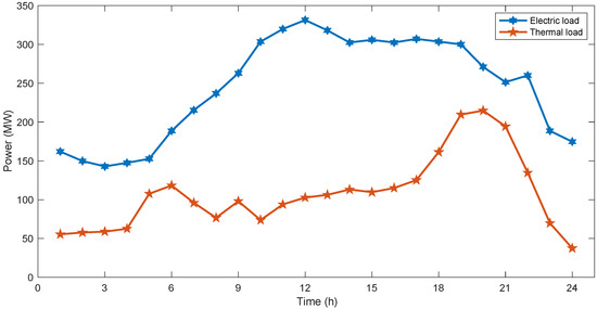
Figure 2.
Electrical load and thermal load data.

Table 1.
Basic parameters.
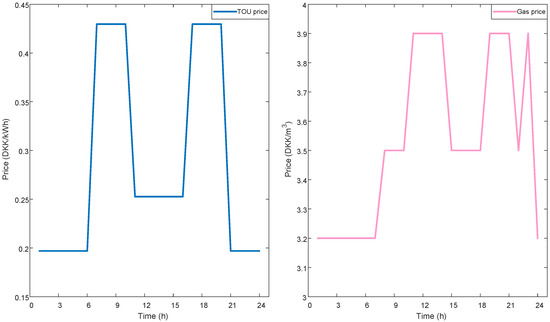
Figure 3.
TOU price and gas price.
This paper uses MATLAB to invoke the YALMIP toolbox to build the model and uses the Gurobi solver to solve it. The dispatching period of the system is 24 h, and the scheduling period is analyzed in the unit of 1 h. To verify the effectiveness of the system and the methods used in this paper, the following scenarios are set, of which Scenario 4 is the optimal dispatching method proposed in this paper.
Scenario 1: The ORC waste heat recovery and demand response are not considered, and the scenario reduction method proposed in this paper is used in the MEVPP system dispatching.
Scenario 2: Consider demand response and use the scenario reduction method proposed in this paper when dispatching the MEVPP system.
Scenario 3: Consider ORC waste heat recovery and use the scenario reduction method proposed in this paper when dispatching the MEVPP system.
Scenario 4: Consider ORC waste heat recovery and demand response and use the scenario reduction method proposed in this paper when dispatching the MEVPP system.
Scenario 5: Consider ORC waste heat recovery and demand response and use the scenario reduction method of K-means when dispatching the MEVPP system.
Scenario 6: Consider ORC waste heat recovery and demand response and use the fast forward reduction method to reduce the scenario when dispatching the MEVPP system.
5.2. Analysis of Basic Operating Results
5.2.1. Reduction of Wind Power and PV Output Scenarios
According to the actual measurement data of wind power and PV in a certain place, 1000 sets of renewable energy output scenarios can be obtained through LHS sampling by adopting the wind power and PV output uncertainty treatment method proposed in Section 3.3. The corresponding reduction scenarios are shown in Figure 4 and Figure 5.
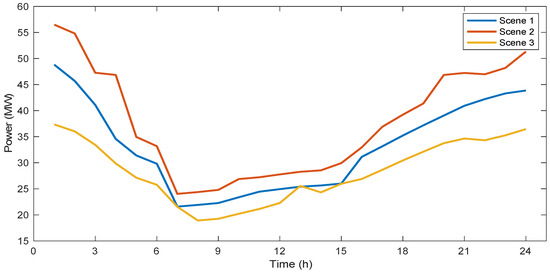
Figure 4.
Scene reduction of wind power output.
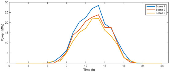
Figure 5.
Scene reduction of PV output.
The wind power and photovoltaic output curves after the reduction are basically consistent with the collective trend before the reduction, which shows that the method proposed in this paper is effective in dealing with the randomness of the wind power and photovoltaic output.
Table 2 shows the results of reducing wind power output by using different parameters.
Table 2.
Operating costs and carbon emission of different scenarios.
It can be seen from Table 2 that the fast-forward reduction method has a longer running time than K-means and the method in this paper. The running time of the K-means clustering algorithm increases significantly with the expansion of scene scale, and the distance after reduction also increases compared with the method in this paper. Compared with other methods, this method reduces the distance before and after scene reduction, improves the reduction accuracy, and is faster than the original reduction method.
5.2.2. Analysis of Dispatching Results of Each Scenario
- Dispatching results of Scenario 1
The dispatching results of the MEVPP system under Scenario 1 are shown in Figure 6. In this scenario, the waste heat of the MT unit is mainly absorbed by the waste heat boiler for heating.
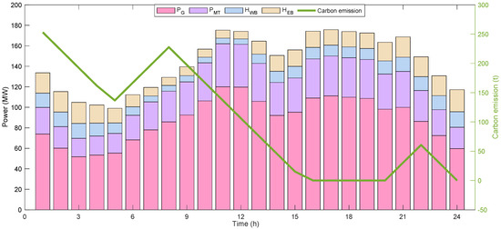
Figure 6.
Power dispatch of the MEVPP system under Scenario 1.
It can be seen from the analysis of Scenario 1 that the capacity of thermal power units limits the carbon capture power plant, and the carbon capture units are at full capacity in periods 10–18. In addition, on the premise of meeting the system operation constraints, the output of other units has also reached the upper limit. It is necessary to extract part of the energy consumption supplied to the carbon capture unit to supply the system power load to maintain the power supply balance of the system. Therefore, most of the output of the carbon capture unit during the peak load period is mainly used to supply the electric load, and only a small part of the output is used to capture carbon. There is a problem of insufficient carbon capture level during the peak load period, which is not conducive to reducing the system’s carbon emissions. At the same time, because the MT unit is restricted by the operation of “power is determined by heat”, it cannot flexibly regulate the system’s power supply balance, which further limits the carbon capture level of the carbon capture power plant.
From the perspective of heat energy supply, the thermal load in the system is preferentially supplied by the waste heat boiler. When the heat energy is insufficient, the gas-fired boiler is called. For example, during periods 2–4, the MT units have less heat due to the influence of thermoelectric coupling, and a gas-fired boiler is used for heating at this time.
EES utilizes its charge/discharge characteristics to realize the time transfer of energy. The operation results of EES are shown in Figure 7.
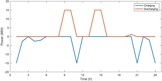
Figure 7.
Operation results of electric energy storage.
First of all, from the charging and discharging curve of electric energy storage, it can be seen that electric energy storage is charged at 1:00–5:00, 11:00 and 21:00–24:00. It can be seen from Figure 3 that the power market price is relatively low at this time. The electric energy storage discharges at times when the power market price is relatively high, such as 9:00–10:00, 14:00–15:00 and 20:00. Thus, the electric energy storage equipment realizes the arbitrage of “low-cost charging and high-cost discharging”, which makes the total cost of the MEVPP system low.
- 2.
- Dispatching results of Scenario 2
In Scenario 2, the electric and thermal demand responses are considered, and the operation results are shown in Figure 8.
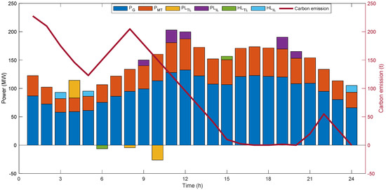
Figure 8.
Power dispatch of the MEVPP system under Scenario 2.
It can be seen from Figure 8 that the energy consumption of the carbon capture unit is reduced in the load reduction periods 9–12 and 19–20. This also shows that the introduction of demand response can effectively reduce the carbon emissions of the system, but the carbon capture unit is still not at the maximum carbon capture level during periods 10–13 and 15–18, and there are still some carbon dioxide emissions.
In addition, during the peak load period, the output of the MT unit increases, and the carbon capture energy consumption of the carbon capture unit further increases. However, due to the limited regulation range of load-side dispatching resources, the carbon capture level still has a large space for improvement.
- 3.
- Dispatching results of Scenario 3
Scenario 4 is to introduce ORC waste heat recovery equipment into the system to supply power to the electrical loads in the system, as shown in Figure 9.
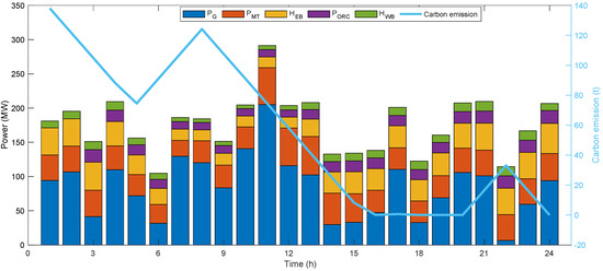
Figure 9.
Power dispatch of the MEVPP system under Scenario 3.
It can be seen from Figure 9 that in the nighttime, due to the poor economy of ORC waste heat power generation, all the thermal power output by the MT unit is used for the heat load supplied by the waste heat boiler. After the introduction of ORC waste heat power generation, the net carbon dioxide emissions are significantly reduced, which indicates that the carbon capture level of the carbon capture unit can be effectively improved by decoupling the operational constraints of “heat determines electricity” of the MT unit. However, due to the capacity of ORC waste heat power generation, the carbon capture unit is also not at the maximum carbon capture level during the period of 15–20. Therefore, the coordination between waste heat power generation and comprehensive demand response should be considered.
- 4.
- Dispatching results of Scenario 4
In scenario 4, the operation of the MEVPP system under the coordination of ORC waste heat power generation and comprehensive demand response is considered, as shown in Figure 10.
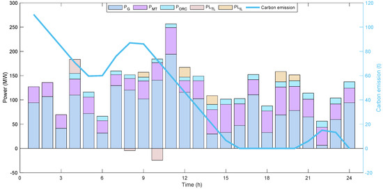
Figure 10.
Power supply and consumption of the system.
In Scenario 4, the dispatching model that comprehensively considers ORC waste heat power generation and comprehensive demand response realizes that the carbon capture unit always maintains the highest carbon capture level, effectively reducing the system’s carbon emissions. At the same time, the residual heat generation capacity of ORC in Scenario 4 is lower than that in Scenario 3 because, after the introduction of a comprehensive demand response, the carbon capture energy consumption deficit of the carbon capture power plant in peak load period is less than that in Scenario 3.
In addition, in order to reflect the flexibility of ORC waste heat power generation to provide MT’s electricity power and thermal output, and then relieve the peak shaving pressure of the system and improve the carbon capture level of the carbon capture unit, Scenario 1 and Scenario 3 are compared and analyzed. During the period when the carbon capture level is insufficient in Scenario 1, the excess heat energy of MT unit in Scenario 4 is used for waste heat power generation through ORC to supply electric load, effectively improving the carbon capture level of the carbon capture unit. The reason for ORC waste heat power generation startup is that it relieves the pressure of system peak shaving, reduces the on-grid power of the carbon capture unit, so that it has sufficient power to supply the carbon capture equipment, and the CO2 captured by the carbon capture equipment is more profitable than the cost of ORC waste heat power generation through the carbon trading market.
- 5.
- Analysis of carbon capture energy consumption in different scenarios
The dispatch of demand response combined with the flexible operation mode of carbon capture power plants has great advantages. For example, the cooperation of the two can realize the flexible and controllable energy consumption of carbon capture and improve the dispatching flexibility of carbon capture units. Figure 11 is a comparison chart of carbon capture energy consumption under different scenarios.
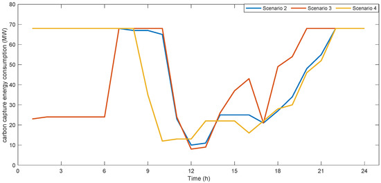
Figure 11.
Comparison of carbon capture energy consumption.
In Scenario 3, the carbon capture unit realizes the energy time shift of carbon capture energy consumption by adjusting the liquid storage capacity. The energy consumption of carbon capture at the peak load is reduced, and the output of high-carbon units is reduced accordingly. When the load is low, the energy consumption of carbon capture increases, which improves its scheduling flexibility and is also conducive to renewable energy consumption.
Compared with Scenario 3, the difference in energy consumption for carbon capture in Scenario 2 and Scenario 4 mainly occurs in the trough period from 1:00 to 6:00, the peak period from 10:00 to 17:00, and some normal periods. This is because the load peak-to-valley ratio will change after demand response, affecting the adjustment plan of carbon capture energy consumption under the original load condition. Compared with Scenario 2 and Scenario 4, the difference is small. The possible reason is that the introduction of an ORC waste heat boiler further reduces the power generation demand during peak hours.
5.3. System Operation Cost Analysis
5.3.1. Breakdown Cost and Carbon Emission Analysis
Through the comparative analysis of Scenario 1 to Scenario 4, this paper aims to illustrate the effectiveness of comprehensive demand response and ORC waste heat power generation in alleviating the problem of insufficient carbon capture level of carbon capture units. The operating costs and carbon emissions of the four scenarios are shown in Table 3.
Table 3.
Operating costs and carbon emission of different scenarios.
From Table 3, comparing Scenario 1 and Scenario 2, it can be seen that after the introduction of a comprehensive demand response in Scenario 2, the system’s total cost is reduced by 1.52%. After considering the comprehensive demand response, due to the improvement of the carbon capture level of the carbon capture power unit, it can capture more CO2 to reduce carbon emissions and thus make profits in the carbon trading market.
Scenario 3 is to introduce ORC waste heat power generation based on Scenario 1. At this time, the total cost of the MEVPP system is reduced by 0.48%. Even though the power generation cost and natural gas cost are higher than those in scenario 1, the carbon capture level of the carbon capture unit is significantly improved, and the profit of the system through the carbon trading market is greater than the increased operating cost of the system.
In Scenario 4, comprehensive demand response and ORC waste heat power generation are considered. The total cost of the MEVPP system is reduced by 2.17% compared with Scenario 1. It shows that the optimal dispatching method proposed in this paper can effectively solve the problem of insufficient carbon capture level of carbon capture units in peak load period and reduce the system operation cost and carbon emissions at the same time.
5.3.2. Cost Analysis of Natural Gas
Through the comparison between Scenario 2 and Scenario 1, it can be seen that since the heat load is all supplied by the gas boiler, and the thermal load and the gas load are the same, the cost of natural gas is basically the same. The natural gas cost in Scenario 3 is 8.3% higher than that in Scenario 1, because the output of MT unit increases after introducing ORC waste heat power generation.
The natural gas cost in Scenario 4 is reduced by 8542 DKK compared with that in Scenario 3. Because the power generation of ORC waste heat recovery equipment is not economical compared with conventional coal-fired units and MT, after introducing a comprehensive demand response, it coordinates with ORC waste heat power generation to optimize MT output. Due to the increase of thermal load, it can directly generate more electric energy, without the need to convert heat energy into electric energy through ORC waste heat power generation, reducing the cascade utilization of energy, improving the energy utilization rate and reducing the cost of natural gas. Therefore, on the basis of Scenario 3, Scenario 4 not only improves the carbon capture level of the carbon capture unit, reduces the carbon emission of the system, but also takes into account the cost of natural gas to minimize the total operating cost of the system.
Although with the improvement of carbon capture level of carbon capture power plants, the cost of coal and gas has increased; that is, more fossil energy is consumed. For example, compared with scenario 1, scenario 4 in this paper increases coal consumption by 0.38% and natural gas consumption by 6.34%, but the benefit of carbon trading has doubled. The carbon emission reduction results obtained are far greater than the value of fossil energy consumed. Therefore, it is worthwhile to obtain low-carbon development and clean energy supply by consuming more and less fossil energy, which is also the necessary stage of the low-carbon transformation of thermal power.
5.4. Sensitivity Analysis
5.4.1. Analysis of Influence of ORC Waste Heat Power Generation Capacity
The above simulation is the system dispatching result considering the ORC waste heat power generation capacity of 25 WM. To prove the rationality of the method proposed in this paper, the changes in the total system cost, natural gas cost and carbon emission under Scenario 3 and Scenario 4 are analyzed when the ORC waste heat power generation capacity is from 5 to 40 MW. Figure 12 shows the total system cost, natural gas cost and net carbon emission under different ORC waste heat power generation capacities. This net carbon emission is the carbon emission of the system participating in the carbon market, that is, the difference between the total carbon emission and the total carbon emission quota.
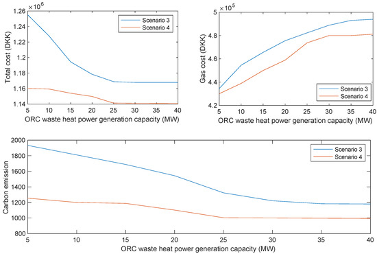
Figure 12.
Sensitivity analysis of ORC capacity.
It can be seen from Figure 12 that with the increase of ORC waste heat power generation capacity, the total system cost and net carbon emission of Scenario 3 and Scenario 4 are in a downward trend. The possible reason is that the increase of ORC waste heat power generation capacity can more effectively decouple the constraint of “determining power by heat”, make MT output more flexible, and improve the carbon capture level of carbon capture power plant. This also proves that the introduction of ORC waste heat power generation in the MEVPP system of carbon capture power unit has a positive effect on saving system costs and reducing carbon emissions.
At the same time, it can be seen from the change in natural gas cost in Figure 12 that with the increase of ORC waste heat power generation capacity, the natural gas cost of the MEVPP system is in an increasing trend. The reason is that the output power source of ORC waste heat power generation is natural gas, and its power is used to increase the energy consumption of carbon capture unit, which is equivalent to using natural gas to generate electricity to supply the carbon capture unit.
5.4.2. Analysis of the Impact of Carbon Trading Price on the Carbon Emissions
Figure 12 is a schematic diagram of system carbon emissions under different carbon trading prices.
It can be seen from Figure 13 that with the increase in carbon trading price, the total carbon emission of the system gradually decreases. When the carbon trading price is lower than 90 DKK, the carbon capture unit is not economical to capture carbon, so the carbon capture unit is not started. When the carbon trading price is between 90–150 DKK, ORC power generation is only started in part of the period to capture CO2. Because the profit of the system through the carbon trading market is less than the cost of natural gas, ORC waste heat power generation is rarely started. With the increase in carbon trading price, the output of ORC waste heat power generation increases, which gradually reflects its economy. This also proves the rationality of introducing ORC waste heat power generation to reduce the carbon emission and total system cost of MEVPP with a carbon capture unit.
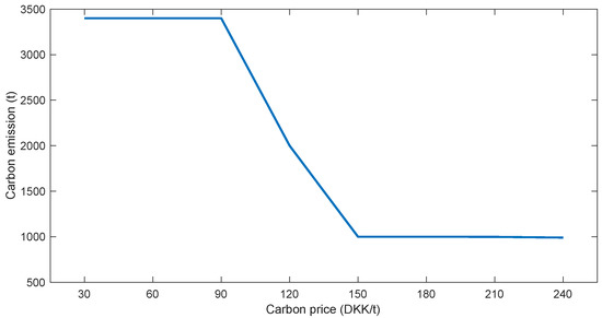
Figure 13.
Total carbon emissions under different carbon trading prices.
Figure 14 is a schematic diagram of the total cost of the system under different carbon trading prices. With the gradual rise of the carbon trading price, the total cost of the system rises first and then falls. When the carbon trading price is 120 DKK, the total cost of the system is the highest. The reason is that when the carbon trading price is lower than 90 DKK, the carbon capture unit does not start. As the carbon trading price rises, the carbon trading cost increases, and the total system cost gradually rises. When the carbon trading price is more than 120 DKK, the profits in the carbon trading market gradually increase due to the low-carbon characteristics of the carbon capture unit, so the total system cost decreases. However, no matter how the carbon trading price changes, the total cost and carbon emissions of the proposed dispatching method are the lowest, proving the proposed method’s effectiveness. To sum up, under different carbon trading prices, the methods proposed in this paper can achieve the comprehensive optimization of low-carbon and economic performance of the system.
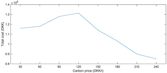
Figure 14.
Total cost under different carbon trading prices.
6. Conclusions
Based on the multi-energy virtual power plant (MEVPP) with a carbon capture unit, this paper builds a dispatching model based on stochastic optimization. The ORC waste heat recovery equipment is introduced at the source side, and the comprehensive demand response is considered at the load side, so that the two can coordinate and cooperate at both sides of the source and load, effectively solving the problem of insufficient carbon capture level of the carbon capture unit during the peak load period. This also considers the low-carbon and economic characteristics of MEVPP and provides a reference for the low-carbon economic dispatching of MEVPP, including carbon capture units. The specific conclusions obtained through the simulation analysis are as follows:
- The cost of MEVPP with the introduction of ORC waste heat power generation equipment is reduced by 1633 DKK, accounting for 0.14%. It has been proved that the introduction of ORC waste heat power generation can decouple the MT unit’s “heat-based electricity” constraint, which is of great significance for the MEVPP of the carbon capture unit.
- Compared with the system without a demand response, the total cost of MEVPP considering a comprehensive demand response is reduced by 21734 DKK, accounting for 1.86%, and 15658 DKK increases the benefit of carbon trading. It is proved that the comprehensive demand response can reasonably adjust the peak-to-valley difference of electricity and heat load and its peak staggering effect, which is of great significance to the realization of low-carbon MEVPP.
- Considering different ORC waste heat power generation capacities and carbon trading prices, sensitivity analysis was carried out on the system’s low carbon and economic situation. The results show that large-capacity ORC waste heat power generation is more conducive to reducing system carbon emissions, but it will increase the cost of natural gas.
In related research in the future, it is necessary to further strengthen the management of the demand side, introduce more refined demand response methods, and consider common load types, such as electric vehicles, to promote the low-carbon operation of the system from both the source and load sides. In addition, for the uncertain factors of the system, it is necessary to actively explore more advanced processing methods, such as robust optimization. The research on robust optimization should focus on the construction of uncertainty sets and strive to reduce the conservatism of the method.
Author Contributions
H.Z.: conceptualization and data curation; C.Z.: writing, software and visualization; Y.Z.: reviewing and supervision; X.W.: reviewing and editing. All authors have read and agreed to the published version of the manuscript.
Funding
This study is supported by the National Natural Science Foundation of China (71973043).
Data Availability Statement
Not applicable.
Acknowledgments
The authors would like to thank the library of North China Electric Power University for its literature support.
Conflicts of Interest
The authors declare no conflict of interest.
References
- Tian, J.; Yu, L.; Xue, R.; Zhuang, S.; Shan, Y. Global low-carbon energy transition in the post-COVID-19 era. Appl. Energy 2022, 307, 118205. [Google Scholar] [CrossRef] [PubMed]
- Naval, N.; Yusta, J.M. Virtual power plant models and electricity markets—A review. Renew. Sustain. Energy Rev. 2021, 149, 111393. [Google Scholar] [CrossRef]
- Ma, Z.; Callaway, D.; Hiskens, I. Decentralized charging control for large populations of plug-in electric vehicles: Application of the Nash certainty equivalence principle. In Proceedings of the 2010 IEEE International Conference on Control Applications, Yokohama, Japan, 8–10 September 2010; IEEE: Piscataway, NJ, USA, 2010; pp. 191–195. [Google Scholar]
- Peridas, G.; Schmidt, B.M. The role of carbon capture and storage in the race to carbon neutrality. Electr. J. 2021, 34, 106996. [Google Scholar] [CrossRef]
- Guo, J.X.; Zhu, K. Operation management of hybrid biomass power plant considering environmental constraints. Sustain. Prod. Consum. 2022, 29, 1–13. [Google Scholar] [CrossRef]
- Yang, Q.; Wang, H.; Wang, T.; Zhang, S.; Wu, X.; Wang, H. Blockchain-based decentralized energy management platform for residential distributed energy resources in a virtual power plant. Appl. Energy 2021, 294, 117026. [Google Scholar] [CrossRef]
- Rahimi, M.; Ardakani, F.J.; Ardakani, A.J. Optimal stochastic scheduling of electrical and thermal renewable and non-renewable resources in virtual power plant. Int. J. Electr. Power Energy Syst. 2021, 127, 106658. [Google Scholar] [CrossRef]
- Sikorski, T.; Jasiński, M.; Ropuszyńska-Surma, E.; Węglarz, M.; Kaczorowska, D.; Kostyła, P.; Leonowicz, Z.; Lis, R.; Rezmer, J.; Rojewski, W.; et al. A case study on distributed energy resources and energy-storage systems in a virtual power plant concept: Economic aspects. Energies 2019, 12, 4447. [Google Scholar] [CrossRef]
- Ghasemi Olanlari, F.; Amraee, T.; Moradi-Sepahvand, M.; Ahmadian, A. Coordinated multi-objective scheduling of a multi-energy virtual power plant considering storages and demand response. IET Gener. Transm. Distrib. 2022, 16, 3539–3562. [Google Scholar] [CrossRef]
- Alabi, T.M.; Lu, L.; Yang, Z. Improved hybrid inexact optimal scheduling of virtual powerplant (VPP) for zero-carbon multi-energy system (ZCMES) incorporating Electric Vehicle (EV) multi-flexible approach. J. Clean. Prod. 2021, 326, 129294. [Google Scholar] [CrossRef]
- Carli, R.; Dotoli, M. A distributed control algorithm for waterfilling of networked control systems via consensus. IEEE Control. Syst. Lett. 2017, 1, 334–339. [Google Scholar] [CrossRef]
- Yan, Q.; Ai, X.; Li, J. Low-Carbon Economic Dispatch Based on a CCPP-P2G Virtual Power Plant Considering Carbon Trading and Green Certificates. Sustainability 2021, 13, 12423. [Google Scholar] [CrossRef]
- Liu, Z.; Zheng, W.; Qi, F.; Wang, L.; Zou, B.; Wen, F.; Xue, Y. Optimal dispatch of a virtual power plant considering demand response and carbon trading. Energies 2018, 11, 1488. [Google Scholar] [CrossRef]
- Ma, Y.; Wang, H.; Hong, F.; Yang, J.; Chen, Z.; Cui, H.; Feng, J. Modeling and optimization of combined heat and power with power-to-gas and carbon capture system in integrated energy system. Energy 2021, 236, 121392. [Google Scholar] [CrossRef]
- Wiesberg, I.L.; de Medeiros, J.L.; de Mello, R.V.P.; Maia, J.G.S.S.; Bastos, J.B.V.; de Queiroz, F.; Araújo, O. Bioenergy production from sugarcane bagasse with carbon capture and storage: Surrogate models for techno-economic decisions. Renew. Sustain. Energy Rev. 2021, 150, 111486. [Google Scholar] [CrossRef]
- Babin, A.; Vaneeckhaute, C.; Iliuta, M.C. Potential and challenges of bioenergy with carbon capture and storage as a carbon-negative energy source: A review. Biomass Bioenergy 2021, 146, 105968. [Google Scholar] [CrossRef]
- Martínez-Sánchez, R.A.; Rodriguez-Resendiz, J.; Álvarez-Alvarado, J.M.; Macías-Socarrás, I. Solar Energy-Based Future Perspective for Organic Rankine Cycle Applications. Micromachines 2022, 13, 944. [Google Scholar] [CrossRef]
- Marefati, M.; Mehrpooya, M.; Pourfayaz, F. Performance analysis of an integrated pumped-hydro and compressed-air energy storage system and solar organic Rankine cycle. J. Energy Storage 2021, 44, 103488. [Google Scholar] [CrossRef]
- Xu, B.; Li, X. A Q-learning based transient power optimization method for organic Rankine cycle waste heat recovery system in heavy duty diesel engine applications. Appl. Energy 2021, 286, 116532. [Google Scholar] [CrossRef]
- Romanos, P.; Al Kindi, A.A.; Pantaleo, A.M.; Markides, C.N. Flexible nuclear plants with thermal energy storage and secondary power cycles: Virtual power plant integration in a UK energy system case study. E-Prime-Adv. Electr. Eng. Electron. Energy 2022, 2, 100027. [Google Scholar]
- Fouskakis, D.; Draper, D. Stochastic optimization: A review. Int. Stat. Rev. 2002, 70, 315–349. [Google Scholar] [CrossRef]
- Wang, X.; Lu, H.; Zhang, Y.; Wang, Y.; Wang, J. Decentralized coordinated operation model of VPP and P2H systems based on stochastic-bargaining game considering multiple uncertainties and carbon cost. Appl. Energy 2022, 312, 118750. [Google Scholar] [CrossRef]
- Carli, R.; Cavone, G.; Pippia, T.; De Schutter, B.; Dotoli, M. Robust Optimal Control for Demand Side Management of Multi-Carrier Microgrids. IEEE Trans. Autom. Sci. Eng. 2022, 19, 1338–1351. [Google Scholar] [CrossRef]
- Melhem, F.Y.; Grunder, O.; Hammoudan, Z.; Moubayed, N. Energy management in electrical smart grid environment using robust optimization algorithm. IEEE Trans. Ind. Appl. 2018, 54, 2714–2726. [Google Scholar] [CrossRef]
- Zhao, H.; Wang, X.; Wang, Y.; Li, B.; Lu, H. A dynamic decision-making method for energy transaction price of CCHP microgrids considering multiple uncertainties. Int. J. Electr. Power Energy Syst. 2021, 127, 106592. [Google Scholar] [CrossRef]
- Aguilar, J.; Bordons, C.; Arce, A. Chance constraints and machine learning integration for uncertainty management in virtual power plants operating in simultaneous energy markets. Int. J. Electr. Power Energy Syst. 2021, 133, 107304. [Google Scholar] [CrossRef]
- Jordehi, A.R. A stochastic model for participation of virtual power plants in futures markets, pool markets and contracts with withdrawal penalty. J. Energy Storage 2022, 50, 104334. [Google Scholar] [CrossRef]
- Zhang, Y.; Liu, F.; Wang, Z.; Su, Y.; Wang, W.; Feng, S. Robust scheduling of virtual power plant under exogenous and endogenous uncertainties. IEEE Trans. Power Syst. 2021, 37, 1311–1325. [Google Scholar] [CrossRef]
- Yan, Q.; Zhang, M.; Lin, H.; Li, W. Two-stage adjustable robust optimal dispatching model for multi-energy virtual power plant considering multiple uncertainties and carbon trading. J. Clean. Prod. 2022, 336, 130400. [Google Scholar] [CrossRef]
Publisher’s Note: MDPI stays neutral with regard to jurisdictional claims in published maps and institutional affiliations. |
© 2022 by the authors. Licensee MDPI, Basel, Switzerland. This article is an open access article distributed under the terms and conditions of the Creative Commons Attribution (CC BY) license (https://creativecommons.org/licenses/by/4.0/).