Article

Modeling and Finite-Horizon MPC for a Boiler-Turbine System Using Minimal Realization State-Space Model

1
College of Automation, Chongqing University of Posts and Telecommunications, Chongqing 400065, China
2
Key Laboratory of Industrial Internet of Things & Networked Control, Ministry of Education, Chongqing University of Posts and Telecommunications, Chongqing 400065, China
3
Institute of Industrial Internet, Chongqing University of Posts and Telecommunications, Chongqing 401122, China
*
Author to whom correspondence should be addressed.
Energies 2022, 15(21), 7935; https://doi.org/10.3390/en15217935
Submission received: 18 September 2022 / Revised: 4 October 2022 / Accepted: 17 October 2022 / Published: 26 October 2022
(This article belongs to the Topic Modeling, Optimization, and Control of Energy Systems)

Abstract

:
This paper aims to address a finite-horizon model predictive control (MPC) for non-linear drum-type boiler-turbine system using a system-identification method. Considering that the strong state coupling of a non-linear mechanism model, the subspace identification method is first utilized to obtain a linear state-space model, and transformed into an input–output model. By taking the inputs and outputs of the input–output model as system states, an augmented non-minimal state-space (NMSS) model of state measurable is constructed. In order to reduce the computation burden, the augmented NMSS model is further transformed into a canonical formulation by adopting a Kalman decomposition. Based on the minimal realization state-space model, the MPC controller is parameterized as a finite-horizon optimization problem. Finally, simulations are performed and evaluated the performance of the proposed method, and the simulation results show that: the linear model approximate the non-linear system accurately; the proposed MPC method can achieve a satisfactory stable control performance; and the computation time 18.388 s for the overall optimization problem also illustrates the real-time performance effectively.

1. Introduction

The thermal power unit, which mainly converts the chemical fuel (e.g., coal, oil, or gas) into electrical energy, is one of the most important energy conversion devices. For a thermal power unit, the fundamental requirement is to guarantee the pressure and water in the drum within the allowable range, while meeting the load demand of electric power. However, the complex dynamic characteristics of the boiler-turbine result in many difficulties for system modeling and control strategy design [1,2,3].
In practice, the operation of thermal power unit combats many challenges, such as severe non-linearity and multivariable coupling, which are the potential causes for the deteriorating performance of stability of thermal power unit. Over the past several decades, in order to eliminate or decrease the effects caused by these problems, plenty of studies have been conducted in industrial and academia; e.g., [4,5,6]. In [4], the authors utilized the fuzzy method to study the modeling problem of a drum-type non-linear boiler-turbine system. The author in [7] investigated the coordinated control problem for boiler-turbine system of coal-fired power plant based on the fuzzy control method. In [8], a multivariable non-linear exponential ARX model was utilized to characterize the non-linear dynamic features of thermal power plants over the whole operating range. The works of [9,10] consider the modeling problem of a thermal power unit which is characterized as a multi-input multi-output radial basis function-based auto-regressive model with exogenous inputs. In fact, these literature show the drawbacks of controlling boiler-turbine system: linearization is made based on the assumption that part of non-linearity can be ignored, complex controller design is not easy to implement, and the simple control methods cannot achieve accurate control.
Model predictive control (MPC), as an advanced control technique proposed by industry circle, has been recognized for an effective and promising method being applied in various fields, ranging from petrochemicals, refining, textiles, and autonomous vehicles (e.g., [11,12,13,14,15,16,17]). In [18], the author designed a robust MPC controller for an automatic voltage regulator against uncertainties. Ref. [19] proposes a heuristic algorithm of MPC to tune the parameters for the robotic manipulator. MPC optimizes an optimal control sequence based on the prediction of future outputs within prediction horizon, and only implements the first control input. The other strength of MPC is that it can directly deal with various hard or soft constraints. Motivated by this outstanding advantage, many researchers have utilized MPC to handle the control problems of thermal power unit (e.g., [6,20,21]). In [6], the authors presented two different step-response models to design dynamic matrix control strategy for a boiler-turbine system. The results showed that, for controller design of the boiler-turbine system, the step-response model based on test data is more effective than a linearized model. In [20], an MPC method merged with the genetic algorithm was introduced to tackle the boiler-turbine control problem. Recently, a hierarchical control framework was proposed in [21] to design an optimal control strategy for a boiler-turbine system, described by the Takagi–Sugeno fuzzy model. The work of [22] considers a fuzzy MPC method for the boiler-turbine system subject to disturbances and uncertainties. Apart from focusing on the engineering problems, some studies also concern the economic and environmental issues of thermal power unit operation. In [2], the authors investigated a hierarchical MPC of a boiler-turbine system which considers the plant-wide economic process optimization and regulatory process control simultaneously. Ref. [23] studies an optimization control method that utilizes MPC for the set-point optimization to improve the safety and economic performance for boiler-turbine system. In [24], from the perspective of scheduling and optimization, the authors presented a zone tracking MPC method, which considers system economic performance during the transient state while always prioritizing unit load demand tracking. Ref. [25] considers the set-point tracking problem for a boiler-turbine unit represented by a non-linear model. In order to obtain an efficient control scheme, the state-space model is on-line linearized at the current operating point, and utilized for prediction and control policy optimization. Unfortunately, the linearized model approach usually assumes that the non-linear part can be ignored, which may cause model mismatch, and results in inaccurate control and performance deterioration. More recently, considering the complexity on the modeling for boiler-turbine system, since artificial intelligence techniques show potential solutions for several complex problems, the academic circle attempt to introduce these techniques, especially in non-linear system modeling [10,26,27] and controller design [28,29,30,31].
In the control literature, there is a abundance of model formulations being utilized in various research directions [32,33,34,35,36], where the state-space model is still the most widely studied models for optimal control, robust control and MPC for its advantage at simplicity implementation of linear system. However, the shortcoming of the state-space model is that it requires states that are measurable when applying the state feedback control, or designs a state estimator when applying the output feedback control. In contrast, the non-minimal state-space (NMSS) model can effectively realize state feedback control by augmenting measured outputs, inputs, and their past values, while avoiding the design of state estimator. Few papers related on NMSS model can be seen in the literature (e.g., [37,38,39,40]). In [39], an improved NMSS-based MPC for multivariable system, which employs a non-zero-pole decoupling approach, was proposed. Based on an augmented NMSS model, the authors in [38] designed a fractional-order MPC strategy for the temperature control model in the industrial heating furnace. For the operation of a boiler-turbine system, an extensive of measurement data can be easily stored and obtained, thus the subspace identification modeling method has been applied for the modeling, multivariable controller design and optimization. In [41], the authors developed a data-driven modeling strategy and designed an MPC controller for boiler-turbine system by dividing the system into several local regions according to the operation range based on the subspace identification and multi-model methods. The subspace identification method is able to estimate the state-space model without non-linear iterative calculation and model parameterization. Despite the identified state-space model widely utilized, their states of these models are meaningless. In order to handle this problem, the idea of augmenting the measured outputs, inputs and their past values of the identified state-space model to construct a NNSS model is a potential approach so that each state variable is measurable or exactly known. Usually, when designing a MPC controller based on an NMSS model directly, the computation burden of MPC optimization problem is large. In fact, utilizing the concept of minimal realization formulation is an alternative approach, but it is rarely reported in the literature. On the other hand, many MPC implementations of NMSS model use heuristic method without stability consideration, this may leads to sub-optimal performance. It is, therefore, necessary to consider optimality to guarantee the control performance, this formulated the main standpoint of this paper.
Motivated by the above discussion, considering the inherent non-linear dynamics of boiler-turbine system and its effect for designing an effective controller, the work hopes to present a clear and intuitive path on how the identification method and MPC can be applied. Consider the influence of non-linear dynamics, we first linearize the non-linear system using an identification method. By adopting the idea of NMSS model and its minimal realization formulation, the state information will be always known and observers are not needed. The main contributions are in the identified model utilized for infinite-horizon MPC (including model minimal realization, terminal control law design, and nominal stability taken into account) and in the unique control structure to achieve good tracking ability, which can be highlighted as follows:
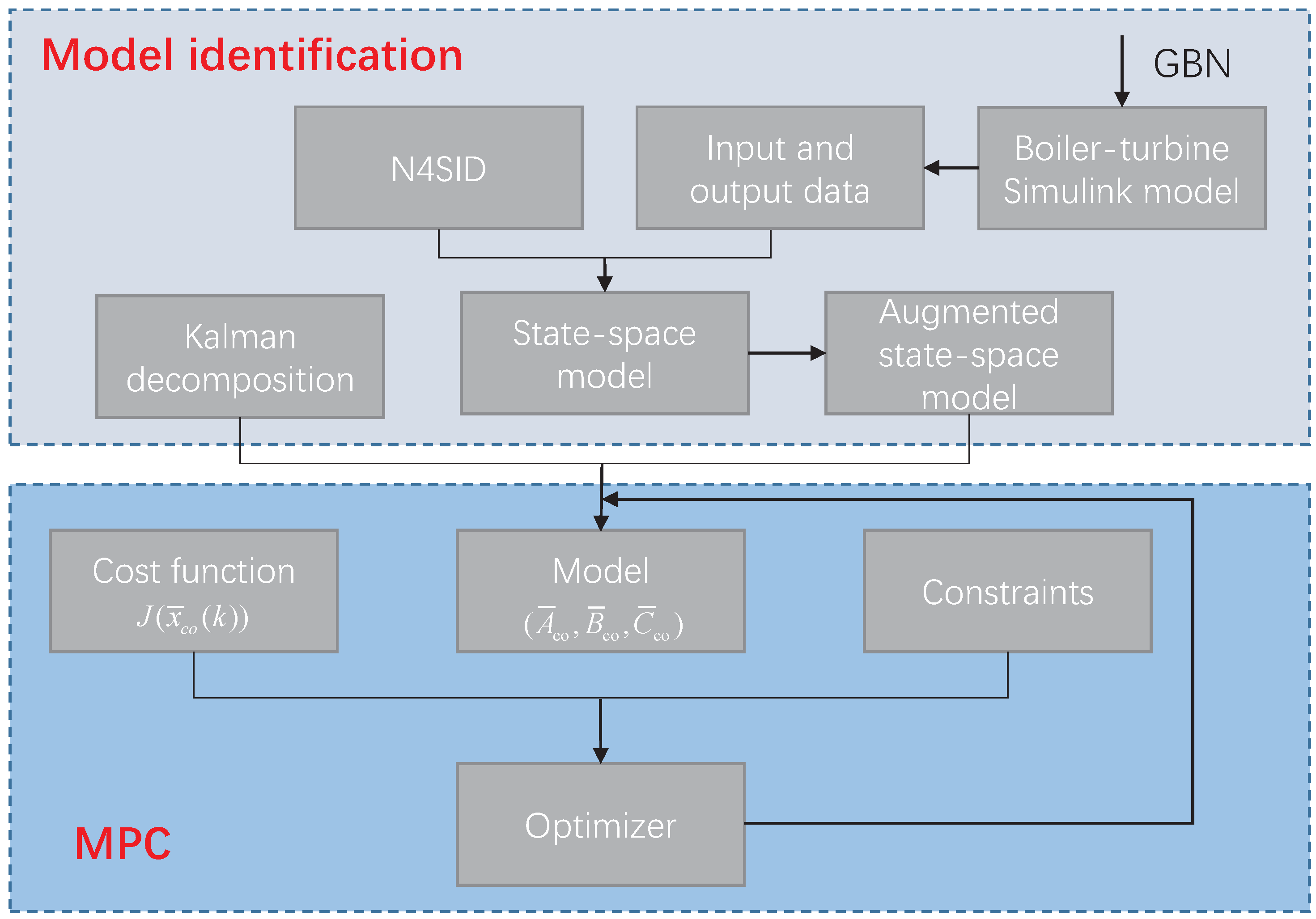
  • The numerical algorithm for subspace state-space identification (N4SID) is utilized for a drum-type boiler-turbine system to obtain a linearized state-space model. By taking the inputs and outputs of the state-space model from the subspace identification method as system states, an augmented NMSS model with state measurable is constructed to avoid a state observer;
  • The augmented NMSS model is transformed into a canonical formulation by adopting a Kalman decomposition in order to reduce the computation burden of controller parameter optimization;
  • Based on the minimal realization state-space model, an MPC controller is transformed into solving a finite-horizon optimization problem, where the cost function is composed by a finite horizon cost and terminal cost. The nominal stability of finite-horizon MPC are also guaranteed for the resulting model.
In the presented control structure, we show a development and combination of MPC and minimal realization model based on previous works [23,42] for a boiler-turbine system. Compared to the literature in [2,23,25,42], the primary novelty and difference of this paper reside in constructing a state measurable, minimal-realization state-space model for the non-linear boiler-turbine system by using identification method to tackle the process non-linearity that the maintains the simplicity of the framework for linear MPC using state-space model, so that the designed MPC controller also has good tracking ability and implementation efficiency.
This rest of this paper is organized as follows. Section 2 shows the facility description of a thermal power unit and its physical process. Section 3 details the identification process of NMSS model. Section 4 presents the finite-horizon MPC method based on NMSS model. Section 5 verifies the effectiveness of the proposed method. Finally, Section 6 summarizes this paper.

2. The Overview for Drum-Type Boiler-Turbine

2.1. Description of the Process

Figure 1 shows a simplified schematic of a drum-type boiler-turbine system that usually includes combustion system, steam-water system, control system, electrical system, condensing system, and so on. The combustion system and steam-water system generate the steam to a certain extent high temperature and pressure. The electric system completes the energy conversion, i.e., realizing the transformation from thermal energy, mechanical energy to electric energy. The control system ensures the safe and economic operation of each subsystem.
The operation process of boiler-turbine system is briefly introduced. Initially, the treated pulverized coal from a coal mill is conveyed to the boiler by belt conveying technology. Pulverized coal is burned in the furnace to heat the boiler in order to convert the water into steam. Steam enters the drum and continues to be heated, and part of steam the high pressure cylinder after primary heating. The drum has the energy store function. When the load changes, it has a certain buffer effect on the imbalance between evaporation and water supply, and rate of change on steam pressure. Steam is reheated in order to improve the thermal efficiency and enters the medium pressure cylinder. Turbine generators are driven by steam from medium pressure cylinders.

2.2. Boiler-Turbine Non-Linear Dynamic Model

In this paper, the classical non-linear model of a 160 MW boiler-turbine generator unit firstly investigated in [43] is considered
x ˙ 1 = 0.0018 u 2 x 1 9 / 8 + 0.9 u 1 0.15 u 3 x ˙ 2 = 0.073 u 2 0.016 x 1 9 / 8 0.1 x 2 x ˙ 3 = 141 u 3 1.1 u 2 0.19 x 1 y 1 = x 1 y 2 = x 2 y 3 = 0.05 0.13073 x 3 + 100 a c s + q e / 9 67.975
where x 1 , x 2 , and x 3 , respectively, represent drum steam pressure, electric power, and fluid density. u 1 , u 2 , and u 3 denote the valve positions for fuel flow, steam control, and feed-water flow, respectively. y 3 is the drum water level determined by
q e = 0.854 u 2 0.147 x 1 + 45.59 u 1 2.514 u 3 2.096 α c s = 1 0.001538 x 3 ( 0.8 x 1 25.6 ) x 3 ( 1.0394 0.0012304 x 1 )
where α c s and q e are the steam quality and evaporation rate, respectively.
In practice, considering the actuators’ manipulate limitation, the inputs are usually required to satisfy the following magnitude constraints:
0 u q 1 , q = 1 , 2 , 3
and have to satisfy the following rate constraints:
0.007 u ˙ 1 0.007 2 u ˙ 2 2 0.05 u ˙ 3 0.05

3. Model Identification Design

The non-linear model (1) properly describes the dynamic characterizes of the boiler-turbine system, however, it encounters great difficulties in controller design due to state coupling interaction and non-linearity. In the sequel, in order to obtain a linear model, the system identification will be utilized to characterize the system dynamic behavior, as shown in the following section.

3.1. Identification Test Signal

We choose the classical generalized binary noise (GBN) proposed by [44] as the test signal. The value of GBN takes a or a. At each predetermined conversion time t, the GBN signal is converted based on the following rules:
Prob { u ( t ) = u ( t 1 ) } = p s w Prob { u ( t ) = u ( t 1 ) } = 1 p s w ,
where p s w denotes the conversion probability. Since the distribution is an independent staggered distribution with probability of p s w at each conversion time t, the mean-value of the signal is 0. The average conversion time is
E T s w = T min p s w ,
where T min denotes the minimum conversion time. It means that the time of GBN signal remains unchanged during the sampling process. The power spectrum of GBN is
Φ u ( ω ) = 1 q 2 T min 1 2 q cos T min ω + q 2 , q = 1 2 p s w .
Remark 1.
Since the plant exhibits severe non-linear dynamics, it is difficult to obtain an accurate linear model using linearization. In order to fully obtain the prior knowledge of process behavior, the plant to be identified should be effectively excited. The excitability conditions of the input signal for the boiler-turbine system (1) are: (a) the signal length should be large enough; (b) the signal changes quickly with a large amplitude, which can generate sufficient excitation to the system. From the generation method of GBN, it can seen that GBN have the merits in setting signal length arbitrarily and having a minimum amplitude factor so that it is available to apply for multivariable model identification.

3.2. Identification and Modeling Performance

Static or steady-state model is utilized to calculate the equilibrium points, which determines operation points and generates set values. For the non-linear model (1), in a steady-state working point, the state variables are constant, therefore,
x ˙ 1 = x ˙ 2 = x ˙ 3 = 0 y 3 = 0
One can calculate several nominal working points based on (1) and (7). In this paper, we consider the case that model (1) represents a 160 MW unit, and the steady-state working points is x eq = [ 115 , 85 , 402.759 ] T , u eq = [ 0.4147 , 0.7787 , 0.5436 ] T , and y eq = [ 115 , 85 , 0 ] T , as shown in [6]. It represents 50 % operation condition. For this working point, the corresponding step-response the non-linear model (1) are plotted in Figure 2.
Based on the non-linear model (1), an open-loop identification experiment is performed to produce the outputs, where Figure 3 shows the state equation in non-linear model (1) using Maltalb Simulink. For the open-loop experiment, the test signal (GBN signal) is set as the process control input. Considering that the rules for test signal stated in Remark 2, choosing the GBN signal follows that: the amplitude should not be too large, and its disturbance to the steady-state operation should be small so that the process variables do not exceed the operation limit. In the identification experiment, since there have three control inputs, we set the sampling time T s = T min = 1 and p s w = 1 / 15 with different amplitude to obtain the open-loop inputs. By these parameter settings, it is able to obtain a good low-pass GBN signal that can fully excite model information. Figure 4 shows a GBN signal utilized in the identification experiment.
Operate the simulation system by superposing the GBN signals in Figure 4 to the respective control valve as control input, it is able to measure and record n = 2500 sets of output data. For the resulting input and output data, it is split into two parts: the first 2000 sets will be utilized for identification, and the rest 500 sets will be utilized for prediction. In this procedure, it takes about 5.889 s for the identification at Matlab R2021a platform with a Intel i7-10700 CPU 2.90 GHz processor.
Based on the first 2000 sets input and output data, the N4SID is applied to estimate the system matrix parameters, mainly including the following two steps: (a) constructing a Hankel matrix based on the input and output data, and performing the singular value decomposition (SVD) on the projection of the Hankel matrix to obtain the estimated state sequence; (b) applying the least square method for the estimated state sequence to obtain system matrices ( A , B , C , D ) . In the identification, the row number of Hankel matrix is set as i = 10 to obtain the distribution of the singular value histogram, as illustrated in Figure 5. It can be seen that the system information mainly distributes in the first three singular values, which indicates the optimal order of the model as n = 3 . Therefore, the resulting identified model is
x ( k + 1 ) = A x ( k ) + B u ( k ) y ( k ) = C x ( k ) + D u ( k )
where the system matrices are
A = 0.9086 0.0266 0.0797 0.1084 0.9915 0.0376 0.0077 0.0217 0.8732 , B = 0.0174 2.5918 0.0190 0.5269 0.0137 0.0768 0.1285 0.0858 0.0616 , C = 0.2205 1.5809 0.4900 8.7136 0.8193 2.4134 0.0047 0.0059 0.0235 , D = 0.1078 0.0177 0.0175 0.0191 0.8039 0.0264 0.2541 0.0958 0.0212 .
In Figure 6, the comparison between of prediction values of controlled variables (CVs) and their real values are plotted. It is shown that the linearized model can accurate behave the non-linear model (1).

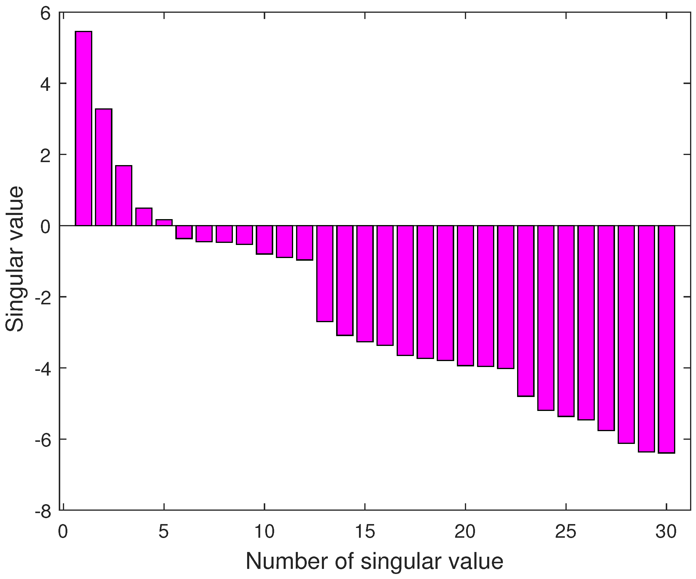
3.3. Minimal Realization NMSS Model

Letting y ( k ) = y ( k ) D u ( k ) , model (8) can be naturally transformed into
x ( k + 1 ) = A x ( k ) + B u ( k ) y ( k ) = C x ( k )
Model (9) can be rewritten as the following input–output model:
A ( z 1 ) y ( k ) = B ( z 1 ) u ( k )
where
A ( z 1 ) = I + a 1 z 1 + + a p z p B ( z 1 ) = b 1 z 1 + + b q z q
where z 1 is the backward shift operator, i.e., z 1 y ( k ) = y ( k 1 ) . a ( z 1 ) and b ( z 1 ) are the matrix polynomials, { a 1 , a 2 , , a p } and { b 1 , b 2 , , b q } are the coefficient matrices with proper dimension. Based on model (10), it is obvious that the order of input and output are n y = n u = 3 . Hence, the coefficient matrices of input–output model (10) are
a 1 = 2.7214 I 3 , a 2 = 2.4734 I 3 , a 3 = 5.623 I 3 b 1 = 0.9673 0.0496 0.7013 0.5216 19.9122 2.0765 0.1258 0.1155 0.0397 b 2 = 0.0397 0.1399 0.6438 1.0945 37.8389 1.8942 0.1236 0.0548 0.0385 b 3 = 0.3278 0.0855 0.1970 0.5278 17.5940 0.5774 0.0403 0.0413 0.0124
Defining the intermediate state vector x n ( k ) = [ y ( k ) , y ( k 1 ) , , y ( k p + 1 ) , u ( k 1 ) , u ( k 2 ) , , u ( k q + 1 ) ] T , model (10) can be rewritten as the following augmented NMSS model:
x n ( k + 1 ) = A n x n ( k ) + B n u ( k ) y ( k + 1 ) = C n x n ( k + 1 )
where
A n = a 1 a 2 a p 1 a p b 2 b q 1 b q I 0 0 0 0 0 0 0 I 0 0 0 0 0 0 0 I 0 0 0 0 0 0 0 0 0 0 0 0 0 0 0 I 0 0 0 0 0 0 0 I 0 , B n = b 1 0 0 I 0 0 T , C n = I 0 0 0 0 0 0 .
Defining a new state vector x ^ ( k ) = [ x n ( k ) , y ( k ) ] T , the augmented NMSS model (11) is reconstructed as
x ^ ( k + 1 ) = A ^ x ^ ( k ) + B ^ u ( k ) y ( k ) = C ^ x ^ ( k )
where
A ^ = A n 0 C n A n I , B ^ = B n C n B n , C ^ = [ 0 I ]
Next, the augmented NMSS model (12) can be rearranged into a canonical form by utilizing a Kalman decomposition that splits the states into following four parts:
  • States which are both controllable and observable;
  • States which are controllable and unobservable;
  • States which are observable and uncontrollable;
  • States which are uncontrollable and unobservable.
By applying controllability and observability transformations on the augmented NMSS model (12), it is shown that the augmented NMSS model (12) is transformed into the following complete Kalman decomposition form:
x ¯ ( k + 1 ) = A ¯ co 0 A ¯ 13 0 A ¯ 21 A ¯ c o ¯ A ¯ 23 A ¯ 24 0 0 A ¯ c ¯ o 0 0 0 A ¯ 43 A ¯ c o ¯ x ¯ ( k ) + B ¯ co B ¯ c o ¯ 0 0 u ( k ) y ( k ) = C ¯ co 0 C ¯ c ¯ o 0 x ¯ ( k )
where x ¯ ( k ) = [ x ¯ co ( k ) , x ¯ c o ¯ ( k ) , x ¯ c ¯ o ( k ) , x ¯ c ¯ o ¯ ( k ) ] T . Therefore, taking the controllable and observable part from the Kalman decomposition yields the following minimal realization state-space model:
x ¯ co ( k + 1 ) = A ¯ co x ¯ co ( k ) + B ¯ co u ( k ) y ( k ) = C ¯ co x ¯ co ( k )
Remark 2.
Identification just determines the model order, but the resulting state vector of identified model (8) are of dimensionless (without physical significance). Augmenting the historic input and output of model (8) as the system state ensures the state variable can be measured and calculated. Transforming the NMSS model into a minimal realization formulation ensures its controllability and observability, which is also helpful to reduce the computation burden and avoid the curse of dimensionality.

3.4. Control Objectives

For the minimal realization model (14), the control objectives are to design an effective controller such that the closed-loop system is asymptotically stable, and the constraints are always satisfied over the control horizon. The two objectives are to be achieved by manipulating the control input u to steer the state to the equilibrium point, while the control inputs are required to maintain a desired range. Since the original non-linear system has been transformed into a linearized model, it ensures that the resulting system state of the linearized NMSS model is measurable. Subsequently, it is easy to design a state feedback-based MPC controller so that the drum pressure y 1 , electric power y 2 , and the drum level y 3 converge to the equilibrium point, which will be illustrated in the sequel.

4. Finite-Horizon MPC Formulation

In order to perform MPC, an optimization problem of the system to be controlled is needed. It includes a prediction model of the physical system and its constraint, as well as a performance function. The following subsections will give the details of designing a finite-horizon MPC for the minimal realization state-space model (14). The proposed control structure is shown in Figure 7. MPC is an advanced computer control technology that on-line optimizes both the current values of control moves and the whole future control sequence over the control horizon. The MPC controller main has three ingredients: prediction model, constraints, and cost function.
Consider the following input and state constraints:
u ̲ u ( k + i ) u ¯ , ψ ̲ Ψ x ¯ co ( k + i + 1 ) ψ ¯ , i 0 ,
where u ̲ : = [ u ̲ 1 , u ̲ 2 , , u ̲ n u ] T , u ¯ : = [ u ¯ 1 , u ¯ 2 , , u ¯ n u ] T , u ̲ j > 0 , u ¯ j > 0 , j { 1 , , n u } ; ψ ̲ : = [ ψ ̲ 1 , ψ ̲ 2 , , ψ ̲ g ] T , ψ ¯ : = [ ψ ¯ 1 , ψ ¯ 2 , , ψ ¯ g ] T , ψ s > 0 , ψ ¯ s > 0 , s { 1 , , g } ; Ψ g × n co .

4.1. Performance Function and Terminal Control Law Design

Consider the following finite-horizon cost function
J ( x ¯ co ( k ) ) = i = 0 N 1 x ¯ co ( k + i | k ) W 2 + u ( k + i | k ) R 2 + x ¯ co ( k + N | k ) P 2 ,
where W, R, and P are the positive-definite weighting matrices; N represents the control horizon. The terminal weighting matrix P is assumed to satisfy [45]
P ( A co + B co F ) T P ( A co + B co F ) + W + F T R F ,
where F is the feedback gain matrix.
Letting X = P 1 , F = Y X 1 and utilizing Schur complement on (17) obtain
X A co X + B co Y X W 1 / 2 X 0 I R 1 / 2 Y 0 0 I 0
Lemma 1
([46]). Suppose that there exist symmetric matrices X = P 1 , { Z , Γ } and matrix Y satisfying (17) and
Z Y T X 0 , Z j j u ¯ j , inf 2 , j { 1 , , n u }
X Ψ ( A co X + B co Y ) Γ 0 , Γ s s ψ ¯ s , inf 2 , s { 1 , , g }
where u j , inf = min { u ̲ j , u ¯ j } , ψ s , inf = min { ψ ̲ s , ψ ¯ s } ; Z j j ( Γ s s ) is the j ( s ) -element of Z ( Γ ) . When x ¯ co ( k + N ) ε P = { z n | z T P z 1 } is satisfied and u ( k + i + N ) = Y X 1 x ¯ co ( k + i + N ) is applied, i 0 , then the closed-loop system is said to be asymptotically stable, x ( k + i + N ) , i 0 always lies inside of ellipsoid ε P , and constraint (15) holds for all i N .
Remark 3.
Since model (14) has a minimal realization formulation, it implies that one can directly state feedback control law, without designing an observer. In Lemma 1, we show the details for designing a terminal control law using model (14) and handling the constraints based on the invariant set. In deriving the inequality from (17) to linear matrix inequality (LMI) (18), it is a congruence transformation that does not introduce any conservatism.

4.2. Overall Optimization Problem and Stability Analysis

The optimal control sequence { u ( k | k ) , , u ( k + N 1 | k ) } is obtained by solving the following finite-horizon MPC optimization problem at each time k:
min u ( k | k ) , , u ( k + N 1 | k ) J ( x ¯ co ( k ) ) ,
s . t . u ̲ u ( k + i | k ) u ¯ , i { 0 , 1 , , N 1 }
ψ ̲ Ψ x ¯ co ( k + i + 1 | k ) ψ ¯ , i { 0 , 1 , , N 1 }
x ¯ co ( k + N | k ) P 2 1 .
The feasible initial state set is a set of initial state points x ¯ co ( 0 ) under the open-loop optimal control sequence { u ( k | k ) , , u ( k + N 1 | k ) } yielded by the optimization problem (21)–(24), such that the system state x ¯ co ( k ) lies in the terminal region ε P at instant k + N , which is defined as
F ( P , N ) = { x ¯ co ( 0 ) n | u ( i ) U , i { 0 , , N 1 } s . t . x ¯ co ( i + 1 ) X , x ¯ co ( N ) ε P } .
Following from the above discussions, the following invariant property result is naturally obtained for optimization problem (21)–(24).
Lemma 2.
Assume that x ¯ co ( k ) F ( P , N ) . There exist κ > 0 and u ( k + i | k ) U , i { 0 , 1 , , N 1 } , such that | u ( k + i | k ) | 2 κ | x ¯ co ( k ) | 2 , x ¯ co ( k + i + 1 | k ) X , i { 0 , 1 , , N 1 } , and x ¯ co ( k + N | k ) ε P .
For the finite MPC, the terminal cost function, the terminal-state region and the terminal control law, shown in the above sections, are the keys to guarantee the close-loop stability. Note that the non-linear system is described by a linear state-space model in the minimal realization formulation, so the nominal stability should be discussed. Based on the presented results, in the following, we will present the stability results of the closed-loop system, composed by model (14) and control moves { u ( k | k ) , , u ( k + N 1 | k ) } .
Theorem 1
(Nominal stability). Suppose that (18)–(20) and x ¯ co ( 0 ) F ( P , N ) are satisfied, then (22)–(24) are always feasible for any k 0 . The closed-loop system is said to be exponential stability by implementing the optimal control input u * ( k | k ) in a receding horizon way.
Proof. 
Suppose that, at each k, the optimal solution for problem is denoted as u * ( k + i | k ) . Based on Lemma 2, a feasible solution at k + 1 can be constructed as
u ( k + i | k + 1 ) = u * ( k + i | k ) , i { 1 , , N 1 } , u ( k + N | k + 1 ) = F x ( k + N | k + 1 )
Considering the invariant property, it is clear that (21)–(24) are feasible for any k 0 . For the purpose of establishing the exponential stability, we should illustrate that there exist a , b , c ( 0 a , b , c ) , such that
a x ( k ) 2 2 J * ( x ( k ) ) b x ( k ) 2 2 , Δ J * ( x ( k + 1 ) ) < c x ( k ) 2 2
where Δ J * ( x ( k + 1 ) ) = J * ( x ( k + 1 ) ) J * ( x ( k ) ) . Once condition (27) holds, then J * ( x ( k ) ) can serve as the Lyapunov function of exponential stability. It is clear that J * ( x ( k ) ) x ( k ) T W x ( k ) λ min ( W ) x ( k ) 2 2 holds, so it is available to choose a = λ min ( W ) . Following from Lemma 2, one has
J * ( x ( k ) ) i = 0 N 1 x ( k + i | k ) W 2 + u ( k + i | k ) R 2 + x ( k + N | k ) P 2 ( N + 1 ) A 2 ( 1 + N B κ ) 2 · max { λ max ( W ) , λ max ( P ) } + N κ λ max ( R ) x ( k ) 2 2
where A = max i { 0 , 1 , , N } A i and κ > 0 . Therefore, it is easy to choose b = ( N + 1 ) A 2 ( 1 + N B κ ) 2 · max { λ max ( W ) , λ max ( P ) } + N κ λ max ( P ) . At time k + 1 , the performance cost is denoted as J ¯ ( x ( k + 1 ) ) under (26), then it is derived that
J * ( x ( k ) ) x ( k ) W 2 + u ( k ) R 2 + J ¯ ( x ( k + 1 ) ) x ( k ) W 2 + u ( k ) R 2 + J * ( x ( k + 1 ) ) .
Inequality (29) shows that Δ J * ( x ( k + 1 ) ) x ( k ) W 2 u ( k ) R 2 λ min ( W ) x ( k ) 2 2 , then it is available to choose c = λ min ( W ) . Hence, J * ( x ( k ) ) is Lyapunov function to prove the exponential stability. The proof is complete. □
Remark 4.
Considering the inherit non-linearity and the optimization mechanism of MPC, it is difficult to obtain the numerical solution of decision sequence { u ( k | k ) , u ( k + 1 | k , , u ( k + N 1 | k ) } even in the case of applying a quadratic performance index. Moreover, the computation burden is always the core issue to be solved. In order to avoid a complex non-linear optimization problem and lead to a large computation burden, we identify the non-linear system to obtain a linear model and transform it into a minimal realization formulation to decrease the system dimension, while guaranteeing fully state measurability and observability.
Remark 5.
For the calculation of identification and controller parameter optimization, error mainly comes from model-mismatch and numerical arithmetic. In the linearization, the non-linear system is assumed to operate a relatively ideal working environment by ignoring isentropic efficiency or isothermal waveforms during the expansion of the working medium in the turbogenerator, this may lead to modeling error during identification process. It is the main reason for affecting the performance of controller. However, the designed MPC applies the feedback control law and optimizes the control sequence in a receding horizon to cope with this error, and maintain good robustness. For the numerical arithmetic, there exists numerical error because of calculation precision.

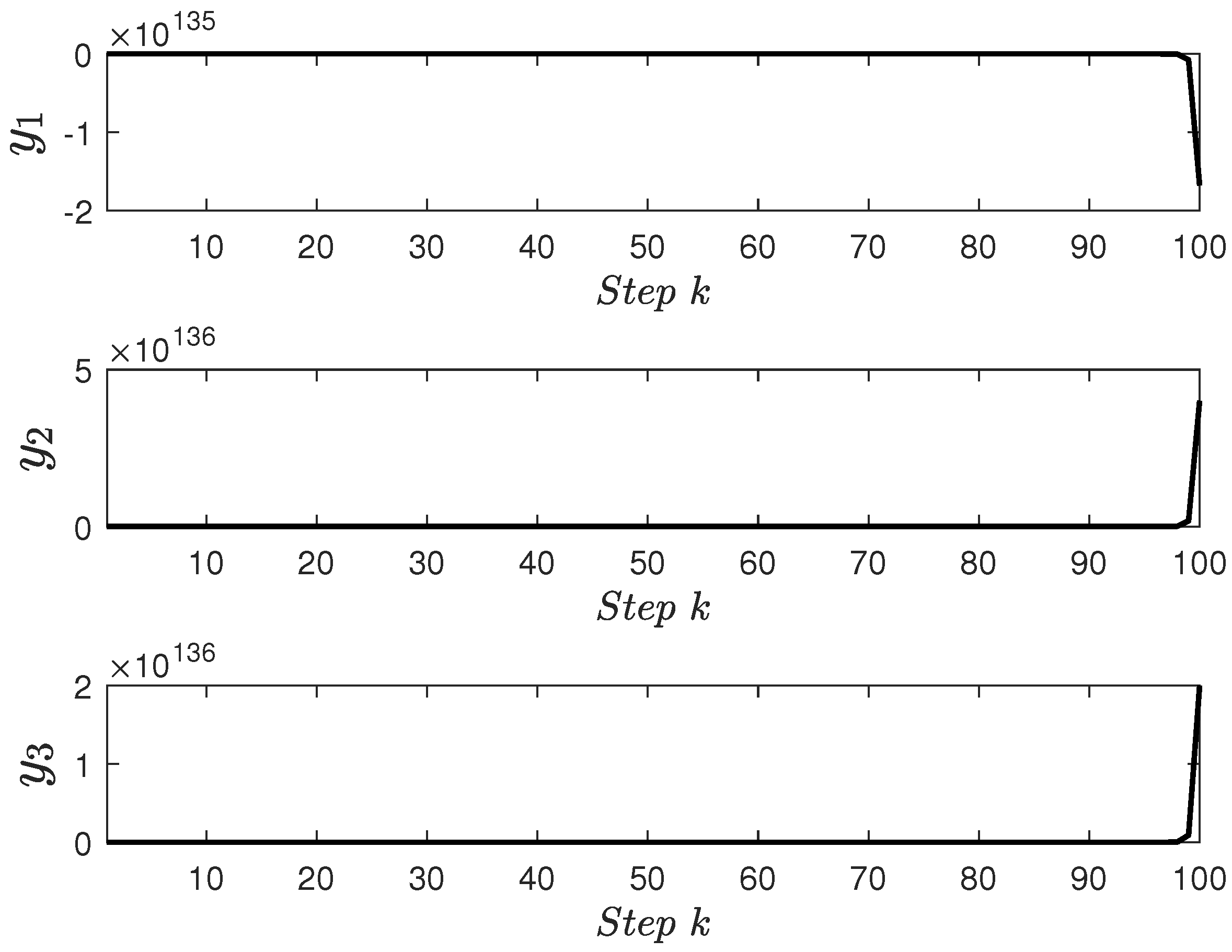
5. Simulation Results and Analysis

This section aims to demonstrate the effectiveness of the finite-horizon MPC based on the minimal realization model (14) and discuss the simulations results to quantify the advantages and disadvantages.

5.1. Simulation Settings

Model described by (14) is utilized for the simulated process. The platform of Matlab 2021a installed on a computer with Intel i7-10700 CPU 2.90 GHz, 16 G RAM is utilized for simulation with a sampling time T s , M P C = 1 .
In the discrete-time domain and MPC implementation, the manganite constraints (2) and the rate constraints (3) on inputs are rewritten as
0 u 1 ( k + i | k ) 1 , i = 0 , , N 0 u 2 ( k + i | k ) 1 , i = 0 , , N 0 u 3 ( k + i | k ) 1 , i = 0 , , N
and
0.007 Δ u 1 ( k + i | k ) 0.007 , i = 0 , , N 1 Δ u 2 ( k + i | k ) 0.02 , i = 0 , , N 0.05 Δ u 3 ( k + i | k ) 0.05 , i = 0 , , N
where Δ u n ( k + i | k ) = u n ( k + i | k ) u n ( k + i 1 | k ) for all n = 1 , 2 , 3 .
Consider the control objective described in Section 3, the following two cases will be presented, so that the results, efficiency and merits of the designed control method are well understood. Case 1 is the scenario for applying classical linear quadratic regulator (LQR) method [47], and Case 2 represent the scenario for applying the proposed control method. In the two cases, both cases take the same weighing matrices W = I , R = I to make a fair comparison.
Case 1.
Since the LQR can not deal with constraints, Equations (30) and (31) will not be imposed.
Case 2.
Based on the resulting minimal realization model { A ¯ co , B ¯ co , C ¯ co } , the following optimization problem is off-line solved
max X , Y t r a c e ( X ) s . t . ( 18 ) ( 20 )
Problem (32) is a standard convex optimization problem that can be directly solved by Yalmip toolbox to obtain X. One has the following terminal weighting matrix
P = 1.1852 0.0051 0.0125 0.1211 0.1697 0.0051 2.3474 0.0809 0.0757 0.1275 0.0125 0.0809 2.7050 0.5774 0.7972 0.1211 0.0757 0.5774 5.2791 0.1514 0.1697 0.1275 0.7972 0.1514 5.4558 .
In Case 2, besides the modeling and constraints, the control parameters should also be set. An important parameter is control horizon N since it affects control quality and computational complexity. Increasing N will improve the optimality, but increases computation burden. For making a balance between optimality and computation, N = 5 is properly determined under several comparison experiments. Based on the above parameter settings, problem (21)–(24) is online solved at each time k to optimize a control sequence { u ( k | k ) , u ( k + 1 | k , , u ( k + N 1 | k ) } , and perform the first control input u ( k | k ) .

5.2. Simulation Results

Closed-loop simulation profiles generated by the two cases are shown in Figure 8, Figure 9, Figure 10, Figure 11, Figure 12 and Figure 13. Following from the responses in Figure 8 and Figure 9, it is obvious that the LQR method can not stabilize model (14). However, the control input signals and output responses of the designed MPC controller plotted in Figure 10, Figure 11, Figure 12 and Figure 13 converge to the steady-state working point. In Figure 10, the constraint of each control action and its rate constraint are always satisfied, this verifies the advantages of MPC at handling physical constraints. Figure 11, Figure 12 and Figure 13 show the outputs (electric power, drum steam pressure, and drum water level) that can eventually maintain stable control by applying the optimal control inputs, respectively. In practice, amplitude constraints have to be considered to guarantee a physical safe operation for the plant, and rate constraints avoids extensive controller parameter tuning. From the comparison, it can be seen that the MPC controller based on the minimal realization state-space model steer the inputs and outputs of the closed-loop system to the equilibrium point, which verify the effectiveness of the proposed MPC. In conclusion, the simulations results illustrate that control performance of MPC controller is superior to a LQR controller.
Further important investigation is to evaluate the performances of the developed models in real-time applications, so we consider the computation complexity of MPC optimization problem. There mainly involve two problems: off-line optimization (32), and online optimization (21)–(24). They are convex optimization problem composed by linear matrix inequalities (LMIs). Usually, the interior point method is applied to solve the feasible solution of LMIs. It is a polynomial complexity algorithm. The complexity is proportional to K 3 L for a given α , where K and L represent the number of scalar LMI variables and the number of scalar rows in LMIs, respectively. It is obvious that the system dimensionality and control horizon affect the complexity of an optimization problem. As stated in Remark 4, the linear model utilized for optimization is transformed into a minimal realization formulation, so we ensure the eventually MPC problem of good efficiency from modeling. In the simulation, the total computation time for carrying out off-line and online stages is 18.388 s. Following the computation time, the implementation efficiency of a linear finite-horizon MPC based on the developed minimal realization model in the real-time performance has been effectively examined.

6. Conclusions

The focus of this paper is to investigate the control problem of the boiler-turbine system based on a system identification method and the finite-horizon MPC. The subspace identification method is firstly employed to obtain a linear state-space model that can properly reflects the dynamic characteristics. By transforming the state-space model into the input–output model and extending its inputs and outputs as a new augmented state, a NMSS model of state measurable is established, and transformed into a minimal realization formulation in order to facilitate state feedback controller and also reduce the computation complexity. A finite-horizon MPC controller, which utilizes a cost function incorporating with a finite-horizon cost and a terminal cost, is designed to guarantee the nominal stability. The physical constraints are handled by an invariant ellipsoid constraint with the terminal control law. Through theoretical proof and comparison simulation, the approach is proven to give an effective control strategy for non-linear system to maintain satisfactory performance as well as a well implementation efficiency. For future works, an interesting plan is to study other issues and make improvements, such as considering the robustness against parametric uncertainty and economic optimization problem.

Author Contributions

Conceptualization, J.W.; methodology, J.W.; software and validation, J.W.; writing—original draft preparation, J.W.; writing—review and editing, B.D.; supervision, P.W. All authors have read and agreed to the published version of the manuscript.

Funding

This research was funded by Natural Science Foundation of Chongqing (No. cstc2021jcyj-bsh0231) and by the Fundamental Research Funds for the Central Universities (No. xzy022019049).

Data Availability Statement

Data sharing not applicable.

Conflicts of Interest

The authors declare no conflict of interest.

Nomenclature

The following abbreviations and symbols are used in this manuscript:
MPCmodel predictive control
NMSSnon-minimal state-space
ARXautoregressive exogenous
N4SIDnumerical algorithm for subspace state-space identification
GBNgeneralized binary noise
SVDsingular value decomposition
CVscontrolled variables
LQRlinear quadratic regulator
LMIslinear matrix inequalities
x 1 ( y 1 ) drum steam pressure ( kg / cm 2 )
x 2 ( y 2 ) electric power ( MW )
x 3 fluid density ( kg / cm 3 )
u 1 fuel flow valve position
u 2 steam control valve position
u 3 feed-water valve position
y 3 drum water level
α c s steam quality
q e evaporation rate ( kg / s )
x eq ( u eq , y eq ) steady-state working (equilibrium) point
p s w conversion probability
Prob { · } the occurrence probability of an event “·”
T s w minimum conversion time
E [ · ] average conversion time
T s w minimum conversion time
Φ u ( · ) power spectrum of GBN
z 1 backward shift operator
n n-dimensional Euclidean space
I n n-dimensional identity matrix
Nprediction horizon
x ( u , y ) state (input, output) vector of identification model
z 1 backward shift operator
x n intermediate augmented state of NMSS model
x ^ system state of NMSS model
A ( B , C , D ) system matrices of identification model
A n ( B n , C n ) system matrices for NMSS model
A ¯ co ( B ¯ co , C ¯ co ) controllable and observable part of NMSS model
x ¯ co system state of minimal realization for NMSS model
Pterminal weighting matrix
W , R positive-definite weighting matrices
u ̲ ( u ¯ ) the lower (upper) bound of input
ε P ellipsoid invariant set
rthe radius of an ellipsoid
x Q 2 x T Q x
h ( k + i | k ) the value of vector h at time k + i , predicted at time k
λ min ( Q ) the minimal eigenvalue of matrix Q

References

  1. Moon, U.; Lee, K.Y. An adaptive dynamic matrix control with fuzzy-interpolated step-response model for a drum-type boiler-turbine system. IEEE Trans. Energy Convers. 2011, 26, 393–401. [Google Scholar] [CrossRef]
  2. Kong, X.; Liu, X.; Lee, K. Nonlinear multivariable hierarchical model predictive control for boiler-turbine system. Energy 2015, 93, 309–322. [Google Scholar] [CrossRef]
  3. Wang, C.; Liu, M.; Zhao, Y.; Qiao, Y.; Chong, D.; Yan, J. Dynamic modeling and operation optimization for the cold end system of thermal power plants during transient processes. Energy 2018, 145, 734–746. [Google Scholar] [CrossRef]
  4. Habbi, H.; Zelmat, M.; Bouamama, B. A dynamic fuzzy model for a drum-boiler-turbine system. Automatica 2003, 39, 1213–1219. [Google Scholar] [CrossRef]
  5. Wen, T.; Marquez, H.; Chen, T.; Liu, J. Analysis and control of a nonlinear boiler-turbine unit. J. Process Control 2005, 15, 883–891. [Google Scholar] [CrossRef]
  6. Moon, U.; Lee, K. Step-response model development for dynamic matrix control of a drum-type boiler-turbine system. IEEE Trans. Energy Convers. 2009, 24, 423–430. [Google Scholar] [CrossRef]
  7. Li, S.; Liu, H.; Cai, W.; Soh, Y.; Xie, L. A new coordinated control strategy for boiler-turbine system of coal-fired power plant. IEEE Trans. Control Syst. Technol. 2005, 13, 943–954. [Google Scholar] [CrossRef]
  8. Peng, H.; Ozaki, T.; Haggan-Ozaki, V.; Toyoda, Y. A nonlinear exponential ARX model-based multivariable generalized predictive control strategy for thermal power plants. IEEE Trans. Control Syst. Technol. 2002, 10, 256–262. [Google Scholar] [CrossRef]
  9. Peng, H.; Wu, J.; Inoussa, G.; Deng, Q.; Nakano, K. Nonlinear system modeling and predictive control using the RBF nets-based quasi-linear ARX model. Control Eng. Pract. 2009, 17, 59–66. [Google Scholar] [CrossRef]
  10. Peng, H.; Kitagawa, G.; Wu, J.; Ohtsu, K. Multivariable RBF-ARX model-based robust MPC approach and application to thermal power plant. Appl. Math. Model. 2011, 35, 3541–3551. [Google Scholar] [CrossRef]
  11. Geyer, T.; Papafotiou, G.; Morari, M. Model predictive direct torque control-part I: Concept, algorithm, and analysis. IEEE Trans. Ind. Electron. 2009, 56, 1894–1905. [Google Scholar] [CrossRef]
  12. Zhang, R.; Sheng, W.; Cao, Z.; Lu, J.; Gao, F. A systematic min-max optimization design of constrained model predictive tracking control for industrial processes against uncertainty. IEEE Trans. Control Syst. Technol. 2018, 26, 2157–2164. [Google Scholar] [CrossRef]
  13. Li, M.; Ping, Z.; Hong, W.; Chai, T. Nonlinear multiobjective MPC-based optimal operation of a high consistency refining system in papermaking. IEEE Trans. Syst. Man Cybern. Syst. 2020, 50, 1208–1215. [Google Scholar] [CrossRef]
  14. Santander, O.; Elkamel, A.; Budman, H. Economic model predictive control of chemical processes with parameter uncertainty. Comput. Chem. Eng. 2016, 95, 10–20. [Google Scholar] [CrossRef]
  15. He, D.; Wang, L.; Yu, L. Multi-objective nonlinear predictive control of process systems: A dual-mode tracking control approach. J. Process Control 2015, 25, 142–151. [Google Scholar] [CrossRef]
  16. Elsisi, M.; Ebrahim, M.A. Optimal design of low computational burden model predictive control based on SSDA towards autonomous vehicle under vision dynamics. Int. J. Intell. Syst. 2021, 36, 6968–6987. [Google Scholar] [CrossRef]
  17. Wang, J.; Ding, B.; Hu, J. Security control for LPV system with deception attacks via model predictive control: A dynamic output feedback approach. IEEE Trans. Autom. Control 2021, 66, 760–767. [Google Scholar] [CrossRef]
  18. Elsisi, M.; Tran, M.; Hasanien, H.; Turky, R.; Albalawi, F.; Ghoneim, S. Robust model predictive control paradigm for automatic voltage regulators against uncertainty based on optimization algorithms. Mathematics 2021, 9, 2885. [Google Scholar] [CrossRef]
  19. Elsisi, M. Optimal design of nonlinear model predictive controller based on new modified multitracker optimization algorithm. Int. J. Intell. Syst. 2020, 35, 1857–1878. [Google Scholar] [CrossRef]
  20. Li, Y.; Shen, J.; Lee, K.; Liu, X. Offset-free fuzzy model predictive control of a boiler-turbine system based on genetic algorithm. Simul. Model. Pract. Theory 2012, 26, 77–95. [Google Scholar] [CrossRef]
  21. Wu, X.; Shen, J.; Li, Y.; Lee, K. Hierarchical optimization of boiler-turbine unit using fuzzy stable model predictive control. Control Eng. Pract. 2014, 30, 112–123. [Google Scholar] [CrossRef]
  22. Morteza, S.; Zahra, R.; Behrooz, R. Fuzzy predictive control of a boiler-turbine system based on a hybrid model system. Ind. Eng. Chem. Res. 2014, 53, 2362–2381. [Google Scholar] [CrossRef]
  23. Klaučo, M.; Kvasnica, M. Control of a boiler-turbine unit using MPC-based reference governors. Appl. Therm. Eng. 2017, 110, 1437–1447. [Google Scholar] [CrossRef]
  24. Zhang, Y.; Decardi-Nelson, B.; Liu, J.; Shen, J.; Liu, J. Zone economic model predictive control of a coal-fired boiler-turbine generating system. Chem. Eng. Res. Des. 2020, 153, 246–256. [Google Scholar] [CrossRef]
  25. awryńczuk, M. Nonlinear predictive control of a boiler-turbine unit: A state-space approach with successive on-line model linearisation and quadratic optimisation. ISA Trans. 2017, 67, 476–495. [Google Scholar] [CrossRef] [PubMed]
  26. Liu, Y.; He, X. Modeling identification of power plant thermal process based on PSO algorithm. In Proceedings of the American Control Conference, Portland, OR, USA, 8–10 June 2005; pp. 4484–4489. [Google Scholar] [CrossRef]
  27. Moon, U.; Lee, K. A boiler-turbine system control using a fuzzy auto-regressive moving average (FARMA) Model. IEEE Trans. Energy Convers. 2003, 18, 142–148. [Google Scholar] [CrossRef]
  28. Kocaarslan, İ.; Ertuğrul, Ç.; Hasan, T. A fuzzy logic controller application for thermal power plants. Energy Convers. Manag. 2006, 47, 442–458. [Google Scholar] [CrossRef]
  29. Liu, X.; Kong, X. Nonlinear fuzzy model predictive iterative learning control for drum-type boiler-turbine system. J. Process Control 2013, 23, 1023–1040. [Google Scholar] [CrossRef]
  30. Strušnik, D.; Avsec, J. Artificial neural networking and fuzzy logic exergy controlling model of combined heat and power system in thermal power plant. Energy 2015, 80, 318–330. [Google Scholar] [CrossRef]
  31. Zhu, H.; Zhao, G.; Sun, L.; Lee, K.Y. Nonlinear predictive control for a boiler-turbine unit based on a local model network and immune genetic algorithm. Sustainability 2019, 11, 5102. [Google Scholar] [CrossRef] [Green Version]
  32. Elsisi, M. Optimal design of non-fragile PID controller. Asian J. Control 2021, 23, 729–738. [Google Scholar] [CrossRef]
  33. Ali, E.; Abd-Elazim, S. BFOA based design of PID controller for two area Load Frequency Control with nonlinearities. Int. J. Electr. Power Energy Syst. 2013, 51, 224–231. [Google Scholar] [CrossRef]
  34. Ismail, M.; Bendary, A.; Elsisi, M. Optimal design of battery charge management controller for hybrid system PV/wind cell with storage battery. Int. J. Electr. Power Energy Syst. 2020, 11, 412–429. [Google Scholar] [CrossRef]
  35. Elsisi, M.; Abdelfattah, H. New design of variable structure control based on lightning search algorithm for nuclear reactor power system considering load-following operation. Nucl. Eng. Technol. 2020, 52, 544–551. [Google Scholar] [CrossRef]
  36. Elsisi, M. Improved grey wolf optimizer based on opposition and quasi learning approaches for optimization: Case study autonomous vehicle including vision system. Artif. Intell. Rev. 2022, 55, 5597–5620. [Google Scholar] [CrossRef]
  37. Wang, L.; Young, P. An improved structure for model predictive control using non-minimal state space realisation. J. Process Control 2006, 16, 355–371. [Google Scholar] [CrossRef]
  38. Zhang, R.; Zou, Q.; Cao, Z.; Gao, F. Design of fractional order modeling based extended non-minimal state space MPC for temperature in an industrial electric heating furnace. J. Process Control 2017, 56, 13–22. [Google Scholar] [CrossRef]
  39. Zhang, J. Improved nonminimal state space model predictive control for multivariable processes using a non-zero-pole decoupling formulation. Ind. Eng. Chem. Res. 2013, 52, 4874–4880. [Google Scholar] [CrossRef]
  40. Wu, S. Multivariable PID control using improved state space model Predictive Control Optimization. Ind. Eng. Chem. Res. 2015, 54, 5505–5513. [Google Scholar] [CrossRef]
  41. Wu, X.; Shen, J.; Li, Y.; Lee, K. Data-driven modeling and predictive control for boiler-turbine unit. IEEE Trans. Energy Convers. 2013, 28, 470–481. [Google Scholar] [CrossRef]
  42. Tao, J.; Ma, L.; Zhu, Y. Improved control using extended non-minimal state space MPC and modified LQR for a kind of nonlinear systems. ISA Trans. 2016, 65, 319–326. [Google Scholar] [CrossRef] [PubMed]
  43. Bell, R.; Åström, K. Dynamic Models for Boiler Turbine Alternator Units: Data Logs and Parameter Estimation for 160 MW Unit; Lund Institute of Technology: Lund, Sweden, 1987. [Google Scholar]
  44. Tulleken, H. Generalized binary noise test-signal concept for improved identification-experiment design. Automatica 1990, 26, 37–49. [Google Scholar] [CrossRef]
  45. Lee, J.W.; Kwon, W.H.; Choi, J. On stability of constrained receding horizon control with finite terminal weighting matrix. Automatica 1998, 34, 1607–1612. [Google Scholar] [CrossRef]
  46. Lee, J. Exponential stability of constrained receding horizon control with terminal ellipsoid constraints. IEEE Trans. Autom. Control 2000, 45, 83–88. [Google Scholar] [CrossRef]
  47. Wei, L.; Fang, F. H-LQR-based coordinated control for large coal-fired boiler-turbine generation units. IEEE Trans. Ind. Electron. 2017, 64, 5212–5221. [Google Scholar] [CrossRef]
Figure 1. Simplified schematic diagram of a thermal power unit including main components.
Energies 15 07935 g001
Figure 2. Step-response of the non-linear system (1) at 50 % operation condition.
Energies 15 07935 g002
Figure 3. The block diagram of state equation in model (1) using Simulink.
Energies 15 07935 g003
Figure 4. GBN signals utilized in the identification experiment.
Energies 15 07935 g004
Figure 5. Singular value histogram.
Energies 15 07935 g005
Figure 6. Prediction value of CVs and their real values.
Energies 15 07935 g006
Figure 7. Proposed framework of MPC based on minimal realization model.
Energies 15 07935 g007
Figure 8. Control inputs of LQR.
Energies 15 07935 g008
Figure 9. Outputs of LQR.
Energies 15 07935 g009
Figure 10. Control inputs of MPC.
Energies 15 07935 g010
Figure 11. Electric power (MW).
Energies 15 07935 g011
Figure 12. Drum steam pressure ( kg / m 2 ).
Energies 15 07935 g012
Figure 13. Drum water level (m).
Energies 15 07935 g013
Publisher’s Note: MDPI stays neutral with regard to jurisdictional claims in published maps and institutional affiliations.

