Buffered Microgrids with Modular Back-to-Back Converter Grid Interface

Abstract

This paper proposes a buffered microgrid with a modular grid interface consisting of a modular back-to-back converter. The proposed method provides a flexible strategy that enables both the load and generation expansion of the microgrid, with no sizing constraints on the initial stage. The method maintains the physical separation of the buffered microgrid from the grid by using back-to-back converters, which ensures a safe, secure and seamless operation in both islanded and grid-connected operation modes. The proposed modular structure allows an energy exchange prioritization either between the energy storage systems and the grid or between the energy storage units themselves, depending on the recommended/desired operational strategy. The prioritizations are achieved by using sets of dead zones in the control of the interfacing converters. In order to control the voltage and frequency, an inverse-droop-based dq-frame current control method was implemented in PSCAD/EMTDC to substantiate the proposed method. The simulation results of different scenarios show the operational flexibility, control simplicity and communication-free operation of the microgrid with different types of sources.

1. Introduction

The proliferation of renewable energy (RE) sources is leading to a shift in electricity generation, where it is connected to distribution networks rather than transmission systems. The distributed nature of such resources, together with energy storage (ES) systems, has led to the creation of distributed energy resources (DERs), which pose several challenges for the operation of power systems. The combination of distributed generation (DG) units, ES and controllable loads has created microgrids (MGs) as a tool to manage and accommodate these components [1,2,3]. Some of the dominant advantages of MGs include operating in both islanded and grid-connected modes, reducing transmission losses and increasing supply reliability by providing local ancillary services [4,5]. Different studies have been conducted to improve the operation of MGs. For example, to overcome the drawbacks of master–slave schemes, the droop control method has been proposed, which is based on measuring the local active and reactive power to set the voltage magnitude and frequency [6,7,8]. In addition, load sharing and ES control have been investigated in several articles [9,10,11,12,13,14], while several other researchers have investigated synchronization issues, particularly at the time of reconnection to the grid [15,16,17]. More recently, to overcome the necessity of an islanding detection algorithm to switch from the grid-connected to islanded mode [18], several control methods have been proposed [19,20,21].

More recent studies have investigated the control and power management of MGs integrated with DERs in light of different connection methods to the main grid. For example, the analysis and control of a back-to-back converter using a multivariable approach were introduced in [22], in which a complicated control system was applied to ensure asymptotic tracking and disturbance rejection. A sag-voltage mitigation scheme based on a modular multilevel converter (MMC) was studied in [23]. The work does not show the capability of the proposed technique to overcome any other operational problems. The sliding mode control technique for a hybrid renewable microgrid is presented in [24]. Although the work presents simultaneous power management between integrated units, it does not show the system’s reaction to critical operating conditions, such as hitting the minimum/maximum SoC or experiencing a sudden change in the load or generation. In References [25,26], the proposed control is based on a multi-agent system and an artificial neural network controller to improve the robust performance of the MG and its control strategy, which imposes further cost and complexity on the system.

Most of the above-mentioned studies suffer from different disadvantages, such as the communication interface, control complexity, operational constraints or additional costs. In addition, most previous articles did not consider all operational scenarios. Moreover, in all previous articles, because of the direct connection between the MGs and the grid, their dynamics and operating conditions (e.g., faults) will affect the other side. To overcome the above-mentioned drawbacks, a buffered MG structure was proposed in [27] that involves the physical isolation of the dynamics of the grid and the MG by using back-to-back converters. The advantages of a buffered MG include its communication-free operation, seamless transitions between all operational modes and applicability to both inductive and resistive loads. In addition, it does not impose any power generation constraints to be applied to DER units and is robust against large load/DG outage disturbances. The operational method proposes a dead zone in the control of the back-to-back converter, which connects the MG to the main grid, giving priority to ES systems to supply/absorb the required/surplus energy. Doing so reduces the energy exchanged with the main grid, and therefore, it reduces the transmission loss. The main drawback is that it proposes bulk converter interfacing without taking the MG’s future expansion into consideration. This imposes a design constraint on the provided solution, which may affect the cost-benefit analysis. In other words, if another unit is added to the MG, the entire interfacing back-to-back converter must be replaced by a larger one.

In this paper, a modular configuration and control paradigm for the interfacing back-to-back converter is proposed to provide a flexible design process, which facilitates the future expansion of the MG without the need to replace the entire interfacing converter. In this structure, for each stage of the MG expansion (not each unit of the MG), a separate set of back-to-back converters will be installed such that the AC sides (on both the grid and MG sides) are connected to a common bus (see Figure 1). Obviously, like any engineering system, the potential future expansion must have been considered in the design stage (e.g., the required physical space should have been allocated). A control paradigm is also proposed that controls the MG-side converters (MGSCs) according to the common local bus voltage level. Cloud-based control implementation is the best option for this structure/control, as it allows for the easy alteration of boundary settings according to different operational priorities/modes. However, the proposed structure/control also works with conventional control implementations.

The advantages of the control scheme and the structure applied to this study over other proposed techniques can be summarized in the following points:

• Communication-free control system. There is no communication interface between the MG and the DERs or the main grid.
• Power generation constraints are applied only when the batteries are fully charged while the MG is islanded.
• The physical isolation between the MG and the main grid protects the MG against grid-side faults.
• Robustness against load and generation disturbances.
• Reduces the energy exchanged with the main grid (because of the proposed dead zone in the control scheme of MGSC and NSC), which reduces the transmission loss.
• Enables coordination between MG units through a central system, if needed.

The advantages of applying the modular back-to-back converter grid interface are:

• It enables easy and economical expansion of the buffered MG, without the need to replace the entire interfacing converter.
• It reduces losses by controlling the MGSCs according to the different levels of the common bus voltage.
• It enables the replacement/repair of one (or more) of the MGSCs without sacrificing the operation of the entire MG.

The rest of the paper is organized as follows. Section 2 presents the proposed system structure and control methodology. In Section 3, PSCAD/EMTDC simulations performed under several scenarios of energy storage integration and fault ride-through are described. The final section of the paper provides concluding remarks on the basic findings of the work.

2. Proposed Structure and Control Method

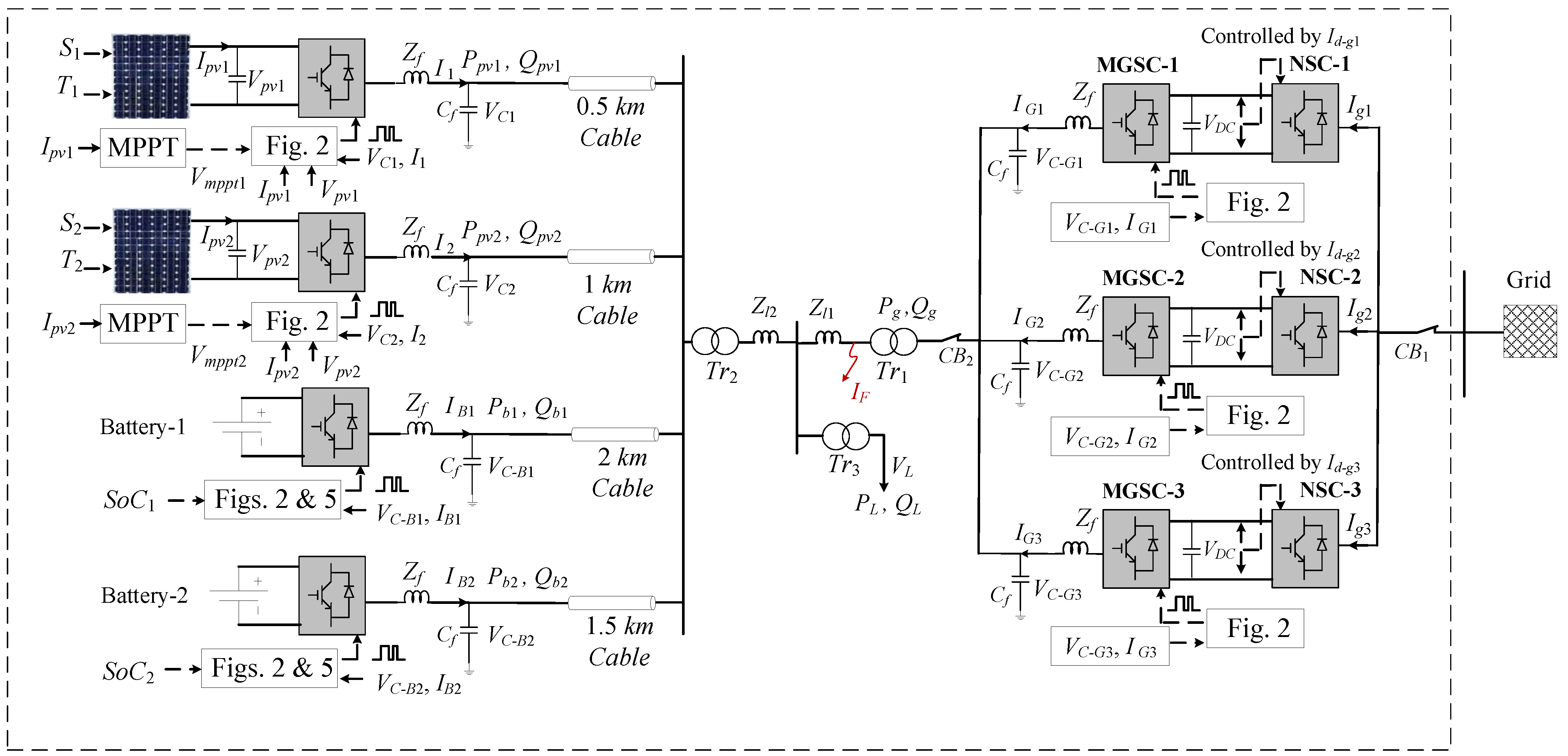
The system under study, shown in Figure 1, consists of an MG connected to an infinite grid through sets of parallel-connected back-to-back converters. The MG consists of photovoltaic (PV) systems and battery ES systems, where each unit is interfaced by a VSC (DC/AC converters) to generate AC power at a voltage level of 11 kV. Two step-up 11/275 kV power transformers are implemented to feed the MG from the DG units’ side and form the main grid side. Taking the space limitation into consideration, three sets of the buffering back-to-back converter, two PV units and two ES units are studied, which allows us to demonstrate their control principles and to present more detailed results. Each of the decoupling back-to-back converters, which consists of an MGSC and a network-side converter (NSC), can be assumed to be one phase of the MG expansion. These three converters are rated at 2, 2 and 1 MVA, able to share 40%, 40% and 20% of the load, respectively. Each of these converters conducts only when needed, as is described later. The PV and ES units are initially set at 5 MVA each, while different ES ratings are considered later in a scenario. It is noted that in this paper, whenever we mention a current per unit (pu), it is based on the unit (PV, ES and converter) rating. However, the power ratings are given pu based on the total system.

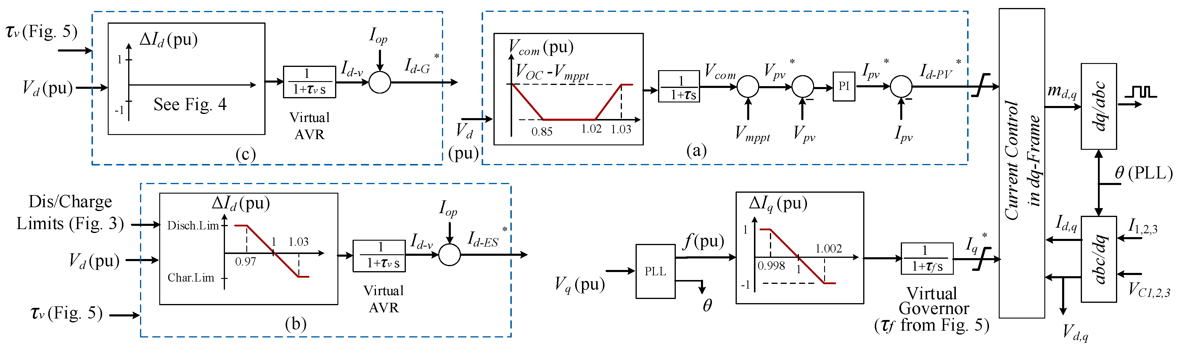
The control principles for the MGSCs, battery converters and PV converters, which are shown in Figure 1 and Figure 2, are very similar, but they have some differences. All of these units are controlled using I_d-V, I_q-f droops to make the system work for both inductive and resistive loads, which is in agreement with the “universal droop” control proposed in [28]. As shown in Figure 1 and Figure 2, local voltages and currents are measured and transformed into a dq-frame (I_d, I_q, V_d and V_q). Each unit is equipped with a Phase-Locked Loop (PLL) that provides the local phase angle θ and frequency f, in addition to synchronizing each DG by regulating local V_q = 0. The per unit (pu) value of the nominal local voltage V_d is calculated during the process, where all converters are current-controlled VSCs using PI controllers. A virtual governor is applied to each unit, i.e., PVs, ESs and MGSCs, which is fed by a locally measured frequency. The virtual governors are identical for all units, providing the reference q-component current I_q^* [18], and use I_q-f droop, described by Equation (1):

$$\mathsf{\Delta }{I}_q{=K}_f \left( f -{ f}_0\right)$$

(1)

where K_f is the droop gain, and f₀ is the nominal frequency (f₀ = 1 pu). Different frequency deviation ranges can be applied, according to different Grid Codes; here, it is set to ±0.2%.

The output of each I_q−f droop is applied to a first-order low-pass filter with a time constant τ_f in order to emulate the damping characteristics of synchronous generators (SGs).

Unlike the virtual governor, which is identical for all types of units, the regulation of active power is different for the integrated generating units, i.e., the PVs, ESs and MGSCs:

PV systems: Since PV arrays do not have any inherent storage capacity (compared to wind turbines), they cannot participate in inertial services. Therefore, the PV system is expected to operate at maximum power point tracking (MPPT) for 0.85 ≤ V_d ≤ 1.02 pu (Figure 1 and Figure 2a). The reference PV-DC voltage $V_{pv}^{*}{=V}_{mppt}{+V}_{com}$, where V_mppt is set by an MPPT algorithm, and the compensation voltage V_com is set by the proposed method, as illustrated in Figure 2a (V_OC is the open-circuit voltage of the PV array):

• For 0.85 ≤ V_d ≤ 1.02 pu, V_com = 0 → $V_{pv }^{*}{=V}_{mppt}$.
• For 0 ≤ V_d < 0.85 pu, V_com increases up to V_OC − V_mppt →${ V}_{pv}^{*}$ increases up to V_OC, which reduces I_pv and $I_{d\text{-}PV}^{*}$. This is a simple Low-Voltage Ride-Through (LVRT) algorithm.
• For 1.02 < V_d ≤ 1.03 pu, V_com increases up to V_OC − V_mppt → $V_{pv}^{*}$ increases up to V_OC, which reduces I_pv and $I_{d\text{-}PV}^{*}$. This is a simple generation shedding algorithm, which will only happen in islanded MGs if P_L < P_PV and the ES is fully charged. Therefore, the generation will be reduced, preventing overvoltage on both the AC and DC sides of the PV inverter.

The limit values of 0.85 pu for LVRT and 1.02 pu for generation shedding are not fixed, and they can be varied with the specific jurisdiction LVRT requirement and the allowed low/overvoltage limits.

ES systems and MGSCs, in principle, use the same I_d-V_d droop characteristic, given by Equation (2):

$$\mathsf{\Delta }{I}_d{=K}_v\left(V_d-V_0\right)$$

(2)

where K_v is the droop gain, and V₀ = 1 pu is the nominal voltage. To emulate the AVR behavior of the SGs, a first-order low-pass filter with the time constant τ_v is used. The d-component voltage V_d is fed to a virtual AVR (Figure 2b,c) to set I_d-v. Then, the reference d-component current will be generated as I_d^* = I_d-v + I_op, where I_op can be used to override the local control (by a centralized system) when coordination between the units is required (e.g., to buy/sell energy). Note that I_op is zero during normal operation.

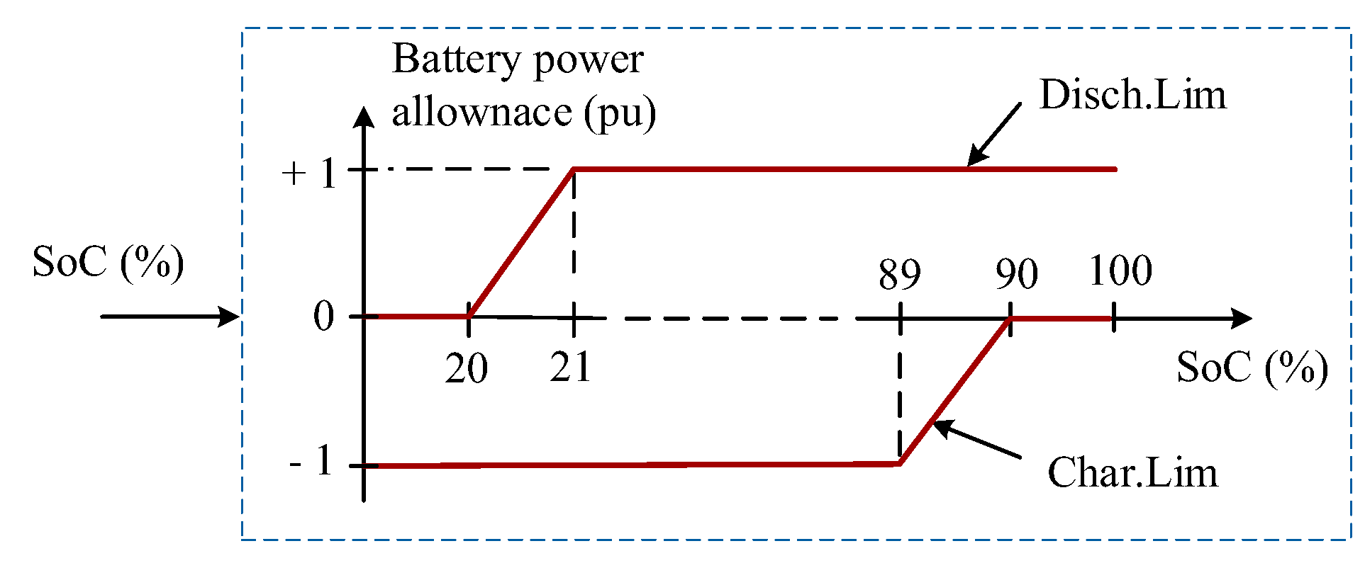
ES systems: The control paradigm for the battery ES systems is illustrated in Figure 2b and Figure 3 (in principle, it is also applicable to other types of ES). In this study, a maximum voltage deviation of ±3% is assumed for both ES units. The I_d-V_d droop characteristics for the virtual AVR are as follows (see Figure 2b):

• In the case of surplus energy, the battery:

Charges proportionally for 1 < V_d < 1.03 pu;

Charges at the maximum level for V_d ≥ 1.03 pu.

• In the case of energy shortage, the battery:

Discharges proportionally for 0.97 < V_d < 1 pu;

Discharges at the maximum level for V_d ≤ 0.97 pu.

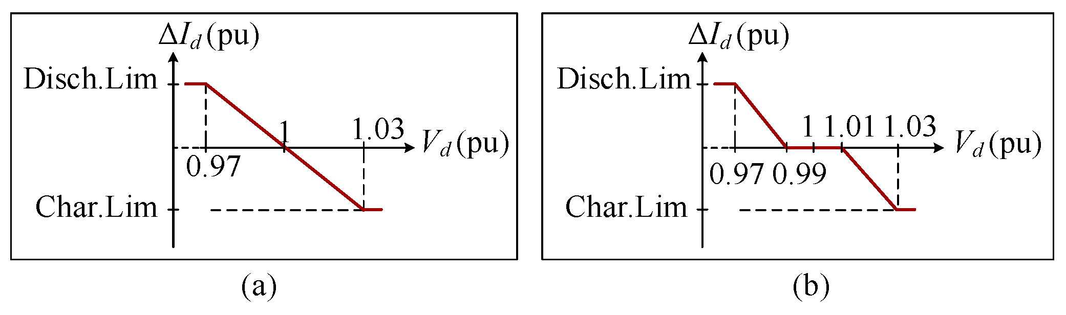
The battery is considered fully charged at SoC 90% and fully discharged at SoC 20%, with charge and discharge limits defined as shown in Figure 3:

• For SoC ≤ 20%, the charge limit = 1 pu and the discharge limit = 0.
• For 20 < SoC < 21%, the charge limit = 1 pu, and the discharge limit varies in a linearly proportional manner from 0 to 1 pu.
• For 21 < SoC < 89%, the charge limit = 1 pu and the discharge limit = 1 pu.
• For 89 < SoC < 90%, the charge limit varies in a linearly proportional manner from 0 to 1 pu, and the discharge limit = 1 pu.
• For SoC ≥ 90%, the charge limit = 0 and the discharge limit = 1 pu.

MGSC control: In general, by controlling the d-component of the MGSC’s current I_d-G, the MGSC absorbs energy from the grid when there is a shortage of energy (V_d < 1 pu) and injects energy into the grid when there is excess energy (V_d > 1 pu). This is reflected in the grid by regulating the d-component of the NSC’s current I_d-g (by controlling the V_DC).

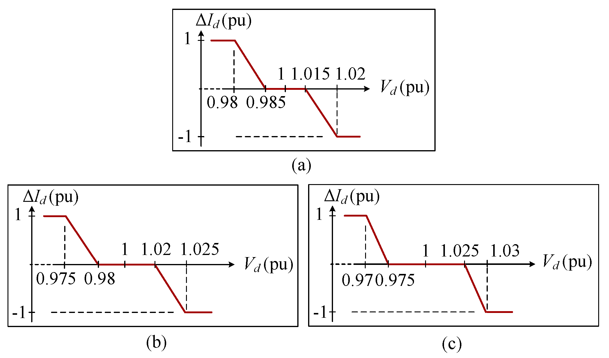
Three different I_d-V_d droop characteristics are used for the AVR of the MGSCs (Figure 2c and Figure 4). All of them are similar in principle (and similar to those of the ES systems), but they are different in their ratings and I_d-V_d droop characteristics, as follows:

• The first MGSC is rated at 2 MVA to allow for a power exchange with the grid up to 40% of the maximum load. It has an I_d-V_d droop characteristic of ±2% voltage deviation, with a dead zone of ±1.5% (Figure 4a).
• The second MGSC is also rated at 2 MVA, but with an I_d-V_d droop characteristic of ±2.5% voltage deviation and a dead zone of ±2% (Figure 4b).
• The third MGSC is rated at 1 MVA (20% of the load), with an I_d-V_d droop characteristic of ±3% voltage deviation and a dead zone of ±2.5% (Figure 4c).

Setting the MGSCs’ I_d-V_d droop in this way enables them to conduct in sequence: i.e., only MGSC-1 conducts if the lack/excess of MG power is up to 2 MVA, while MGSCs-2 and -3 start contributing when this power exceeds 2 and 4 MVA, respectively. This approach minimizes converters’ loss in the proposed modular configuration. Note that the dead-zone margins can be changed or even removed according to the converters’ sizes and the desired operational strategy. The expansion of the MG (an increase in demand/generation) can be met by adding a new parallel set/sets of back-to-back converters with the required capacities and suitable dead-zone margins to enable a flexible operation. This approach works best with a cloud-based control paradigm, where the stings can be updated by the operators.

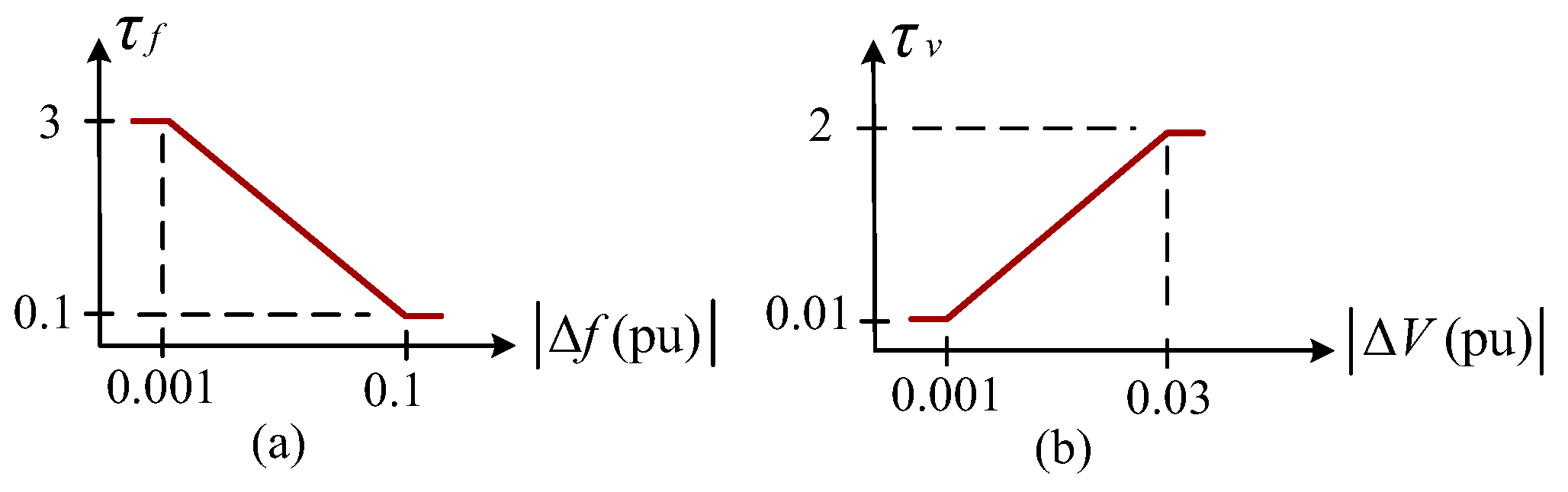
A dynamic method to set τ_f and τ_v is proposed, as shown in Figure 5. It can be seen that at steady state (small voltage and frequency deviations), the damping factor would increase for higher τ_f, while to provide an accelerated active power service, a small τv is needed. Therefore, the system damping increases by reducing τ_f if ΔV and Δf increase. On the other hand, an increase in τv is required for oscillation suppression. The slope and limits of τ_f and τ_v vary depending on the requirements for the response dynamics and damping.

3. Simulation Results

To illustrate the performance of the proposed scheme, the system shown in Figure 1 was simulated, and different scenarios were implemented using PSCAD/EMTDC. The system parameters are given in Table 1, and the MPPT algorithm presented in [29] was applied in this study (other MPPT methods could also be applied).

The load model is described by Equations (3) and (4), which is a ZIP model that reflects a combination of constant impedance, constant current and constant power loads [30]:

$$P_L{=P}_0\left[a_1{\left(\frac{V}{V_0}\right)}^2{+a}_2\left(\frac{V}{V_0}\right){+a}_3\right]$$

(3)

$$Q_L{=Q}_0\left[a_4{\left(\frac{V}{V_0}\right)}^2{+a}_5\left(\frac{V}{V_0}\right){+a}_6\right]$$

(4)

where:

• V₀, P₀ and Q₀: nominal values for voltage, load active power and load reactive power, respectively.
• a₁, a₂ and a₃: active power factors for constant-impedance, constant-current and constant-power loads, respectively.
• a₄, a₅ and a₆: reactive power factors for constant-impedance, constant-current and constant-power loads, respectively.

The coefficients a_1–6 were determined in [31] for industrial, commercial and domestic loads. The average coefficients of those investigated in [31] are used in this paper, i.e., a₁ = 0.98, a₂ = −1.19, a₃ = 1.21, a₄ = 6.32, a₅ = −10.27 and a₆ = 4.95.

Table 1. Parameters of the simulated system.

Component	Parameter	Value	Unit
275 kV Transmission Lines [32]	Rl	30	mΩ/km
	Ll	1	mH/km
	Cl	10	nF/km
Power Transformers [32]	Xl	0.02	pu
11 kv, 185 mm2 XLPE Cables [33]	Rc	0.131	Ω/km
	Lc	0.29	mH/km
	Cc	0.38	μF/km
Filters	Rf	0.5	mΩ
	Lf	3.852	mH
	Cf	6.577	μF

Table 1. Parameters of the simulated system.

Component	Parameter	Value	Unit
275 kV Transmission Lines [32]	Rl	30	mΩ/km
	Ll	1	mH/km
	Cl	10	nF/km
Power Transformers [32]	Xl	0.02	pu
11 kv, 185 mm2 XLPE Cables [33]	Rc	0.131	Ω/km
	Lc	0.29	mH/km
	Cc	0.38	μF/km
Filters	Rf	0.5	mΩ
	Lf	3.852	mH
	Cf	6.577	μF

Please note that because the MG has a buffered structure, a black-start operation is inherently investigated in all of the following scenarios. It is also emphasized again that the current pu values are based on each unit’s rating, while the power pu values are given based on the total system (5 MVA).

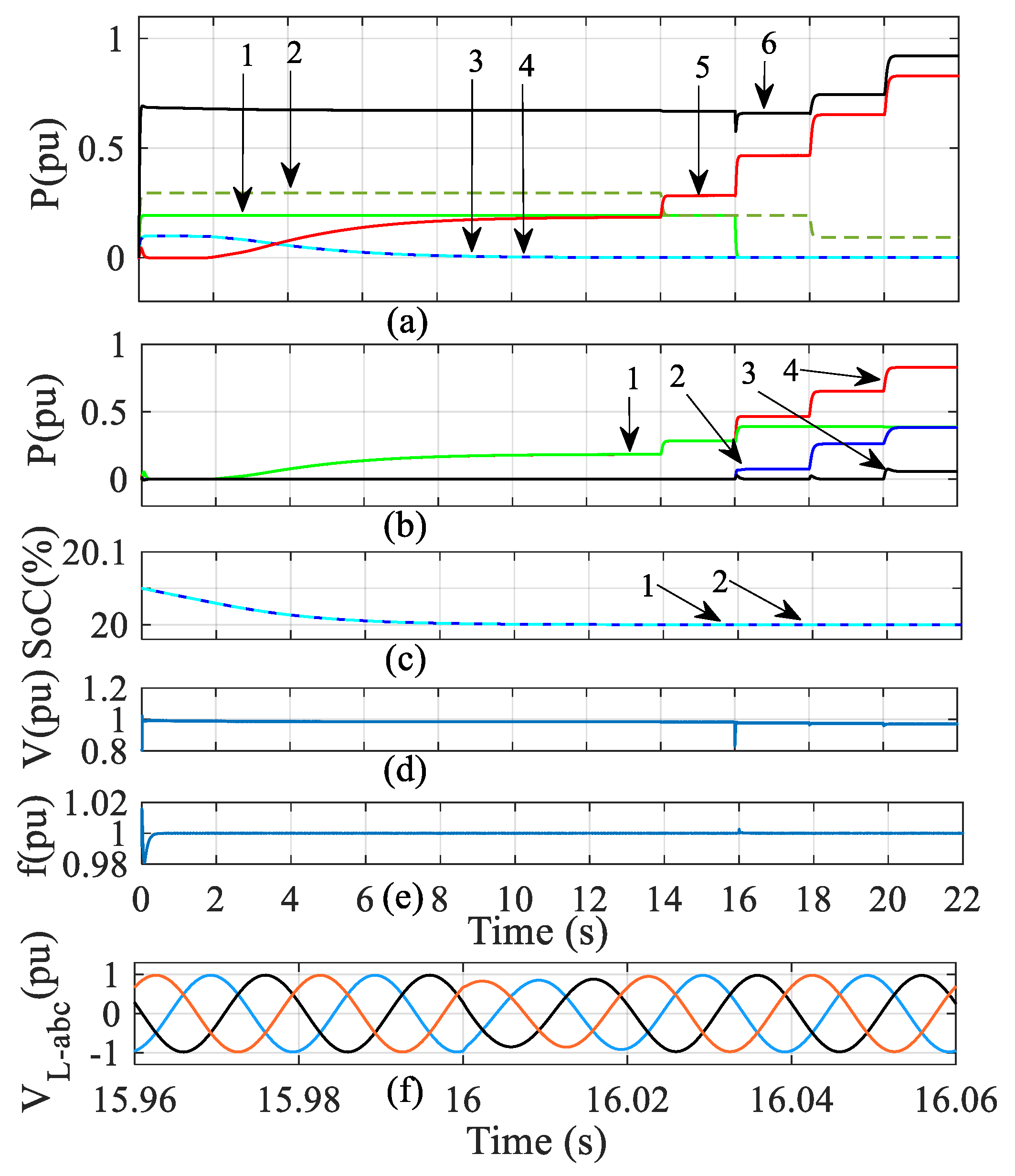
3.1. Reaching Min. SoC Limit, Sudden Load Change and Sudden Generation Loss

This scenario was designed to investigate the robustness of the proposed control scheme against several events, including reaching the minimum SoC, a sudden large change in the load and a sudden large loss of generated PV power. The sequence of these events is as follows:

The initial settings are P_pv1 = 0.2 pu, P_pv2 = 0.3 pu and P_L = 0.7 pu; the two batteries have the same rating, and their SoCs are set slightly above their minimum limit of 20%. Since the total P_pv < P_L and SoC > 20%, P_g = P_g1 + P_g2 + P_g3 = 0 pu, and the lack of generation is covered by the two batteries equally. At t ≈ 6 s, the batteries’ SoCs reach 20% (Figure 6c); therefore, P_b1 + P_b2 declines to zero (Figure 6a), which makes MGSC-1 conduct seamlessly (P_g1 = 0.2 pu) to compensate for the power shortage (Figure 6b). At t = 14 s, a 10% reduction in P_pv2 = 0.2 pu makes MGSC-1 compensate for this power shortage (P_g1 = 0.3 pu). At t = 16 s, PV₁ is disconnected, resulting in a sudden generation loss of 20% (P_pv1 = 0 pu). The 20% power loss is seamlessly balanced by MGSC-1 (i.e., P_g1 = 0.4 pu, which is its maximum capacity) and MGSC-2 (P_g2 = 0.1 pu). At t = 18 s, the load increases to P_L = 0.8 pu, and PV generation decreases to P_pv2 = 0.1 pu, which makes MGSC-2 cover the power shortage (P_g2 = 0.3 pu).

At t = 20 s, a sudden large load increase of 20% takes place, which makes MGSC-2 reach its maximum rating (P_g2 = 0.4 pu), and MGSC-3 conducts seamlessly to cover the remaining needed power (P_g3 = 0.1 pu). It can be seen in Figure 6a,b that all MGSCs seamlessly contribute to react to the power changes. Figure 6d,e show that the load voltage magnitude and frequency are within their statutory limits [34], respectively. Figure 6f shows how fast the load voltage is recovered after a sudden 20% generation loss at t = 16 s.

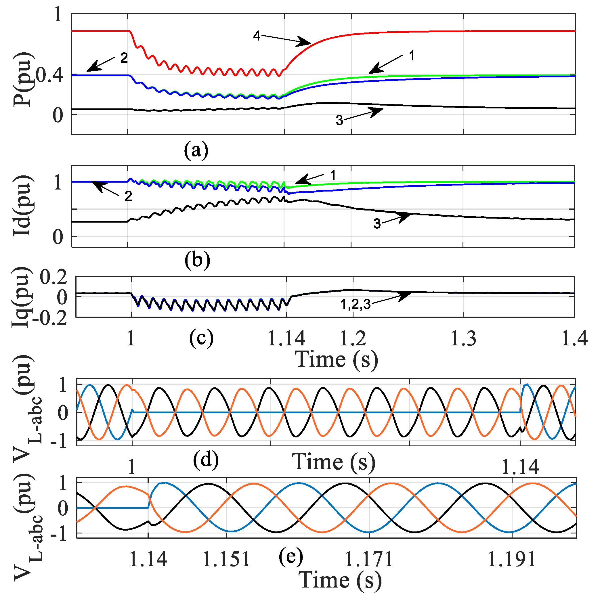
3.2. Fault Ride-Through Capability

To examine the fault ride-through (FRT) capability of the proposed modular structure, symmetrical and asymmetrical faults were applied to the MG (I_F in Figure 1).

(1)

Single-line-to-ground fault

In this scenario, all three MGSCs are assumed to be conducting to examine their behavior under a fault; i.e., the load is fed only from the grid.

To do so, P_pv1 = P_pv2 = 0 pu, the batteries’ SoCs are set at 20%, and thus, P_b1 = P_b2 = 0 pu. P_L = 0.9 pu; therefore, P_g1 = P_g2 = 0.4 pu (at their maximum capacity) and P_g3 = 0.1 pu. A single-line-to-ground (SLG) fault is applied (I_F in Figure 1) at t = 1 s to be cleared after 140 ms. Figure 7a shows that the power contribution of the three MGSCs remains stable after the fault is cleared. Figure 7b,c show the d- and q-components of the converters’ currents, respectively. It can be seen in Figure 7b that MGSC-1 and MGSC-2 are at their full capacity of 1 pu (based on their own ratings). Figure 7d shows that the two healthy phases have a sinusoidal voltage during the fault, whereas Figure 7e shows that the load voltage rise after the fault is cleared is under 0.3 pu, and the frequency is restored within two cycles, which is within the operational recommendations of the power system [35].

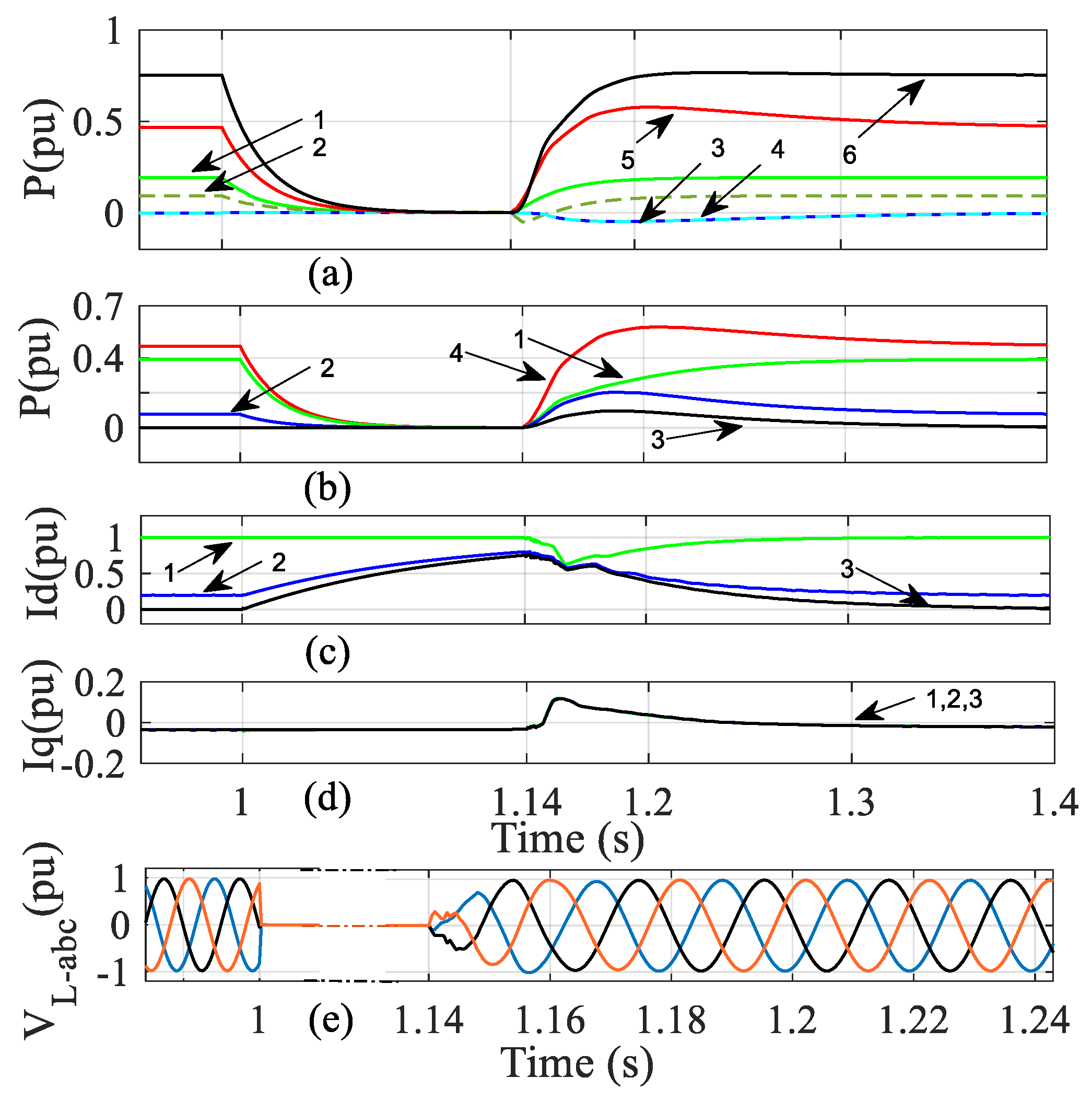
(2)

Three-phase-to-ground fault

In this scenario, a three-phase-to-ground fault is applied at t = 1 s to be cleared after 140 ms. Unlike the SLG fault, where the load is fed from the grid only, in this scenario, the PV units participate in feeding the load in order to examine the fault effect in such a case (P_pv1 = 0.2 pu and P_pv2 = 0.1 pu). The batteries’ SoCs are set at 20%; thus, P_b1 = P_b2 = 0 pu. P_L = 0.8 pu, and therefore, P_g1 = 0.4 pu (its maximum power rate) and P_g2 = 0.1 pu (the remaining power needed to cover the load). Figure 8a shows that power sharing remains stable after the fault is cleared. Figure 8b shows that the power contribution of the MGSCs remains constant as well. Figure 8c,d show the d- and q-components of the converters’ currents, respectively. Figure 8e shows that the voltage rise is under 0.3 pu, and the frequency is restored within three cycles, which is within the operational recommendations of the power system.

3.3. Hitting Max. SoC Limit of the Batteries

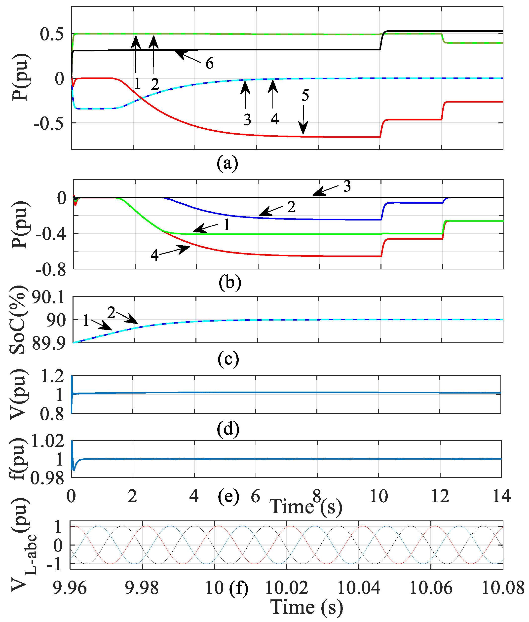
In this scenario, the behavior of the proposed modular configuration is examined when the MG possesses an energy excess. The events of this scenario are as follows:

The SoC limit of both batteries is set slightly below 90% (their maximum limit). P_pv1 = P_pv2 = 0.5 pu and P_L = 0.3 pu (i.e., 0.7 pu overgeneration). Initially, the two batteries absorb the energy excess equally (since they have the same ratings), and thus, P_g = 0 pu, as shown in Figure 9a. At t ≈ 1.5 s, the batteries are close to fully charged; therefore, MGSC-1 seamlessly starts to conduct (Figure 9b), exporting the extra energy to the grid.

When the surplus of the energy reaches 0.4 pu (the maximum capacity of MGSC-1), MGSC-2 seamlessly starts to conduct, transmitting the energy excess to the grid (note P_g3 = 0). At t ≈ 6 s, both batteries are fully charged (Figure 9c), and the whole energy excess is transmitted to the grid. At t = 10 s, a sudden large load increase takes place, P_L = 0.5 pu, which is reflected in the power transmitted through MGSC-2 only because the total amount of the excess power is still higher than MGSC-1 (i.e., 0.4 pu). At t = 12 s, P_pv1 = P_pv2 = 0.4 pu. Now, because P_pv1 + P_pv2 − P_L < 0.4 pu (i.e., P_g1-Max), only MGSC-1 conducts (P_g2 = 0 pu). Figure 9d,e show that the voltage magnitude and frequency are well-controlled during all of the events’ changes in this scenario. Figure 9f shows the zoomed-in three-phase load voltage at the time of the sudden 20% load increase (t = 10 s) to demonstrate the accuracy of the measured voltage and frequency.

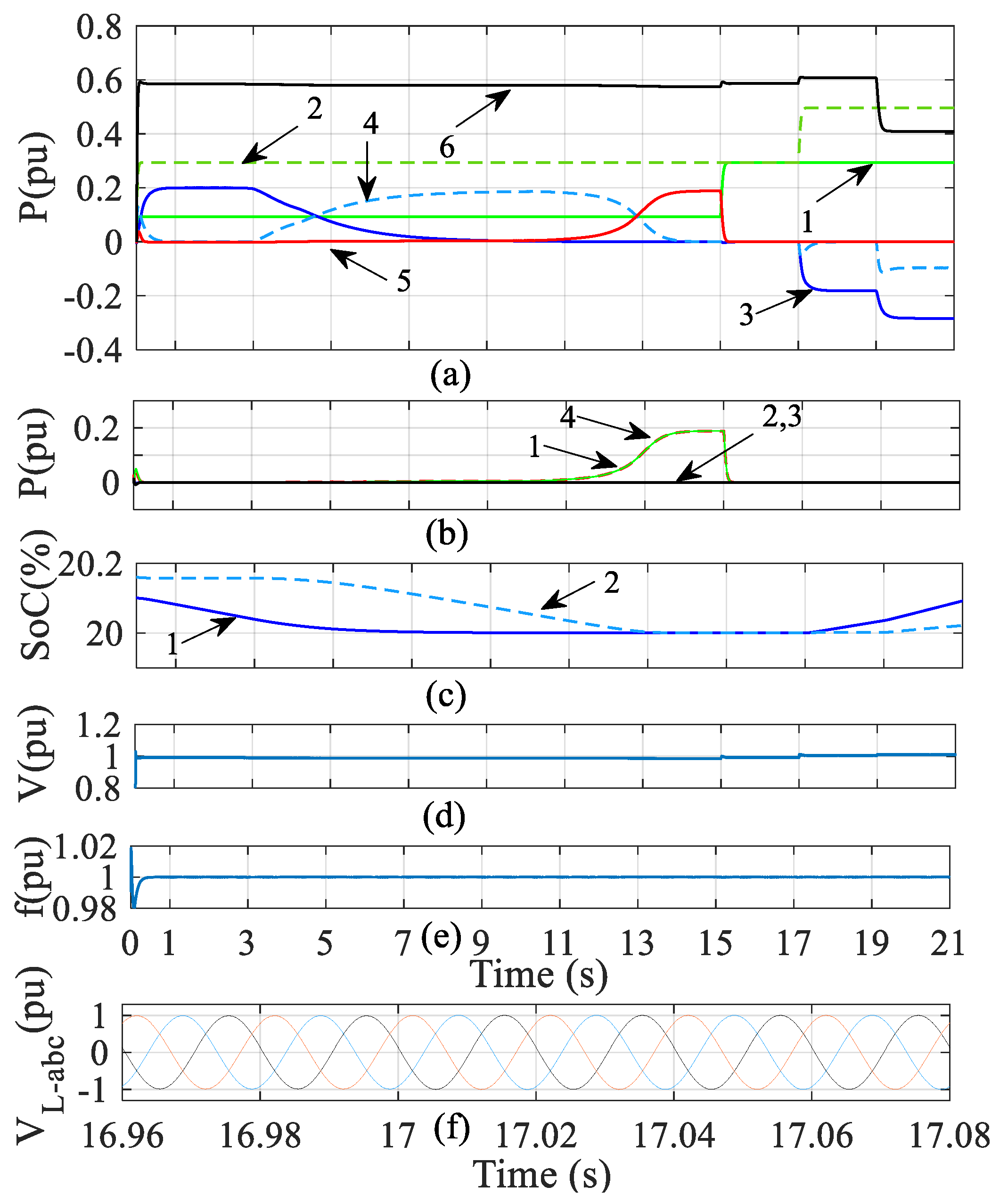
3.4. Prioritizing Operation between ES Units

In contrast to the previous scenarios, the two ES units are assumed to have different ratings in this scenario: i.e., ES-1 is set to 1.5 MVA (0.3 pu), and ES-2 is 2.5 MVA (0.5 pu). In addition, a charge/discharge priority is given to ES-1 over ES-2. This could be integrated into a practical application when one of the ES units (here, ES-2) suffers from a degradation issue. Therefore, the network operator wants to reduce its charge/discharge cycles to save its state of health until scheduled maintenance is due. To do so, a dead zone in the I_d-V_d droop characteristic of the ES-2 unit is implemented, as shown in Figure 10. The events of this scenario are as follows:

Initially, P_pv1 = 0.1 pu, P_pv2 = 0.3 pu and P_L = 0.6 pu. Therefore, the 0.2 pu shortage is compensated for by the batteries, while P_g1 = P_g2 = P_g3 = 0 pu. The SoCs of the two batteries are set to be different and a bit higher than their minimum limit of 20%.

As can be seen in Figure 11a, although SoC₂ > SoC₁, only ES-1 conducts because it has a charge/discharge priority (ES-2 has a dead zone), P_b1 = 0.2 pu and P_b2 = 0 pu. At t ≈ 3 s, the SoC of ES-1(SoC₁) is close to 20%, and ES-2 starts to conduct, as shown in Figure 11a,c.

At t ≈ 8 s, ES-1 is fully charged, and only ES-2 conducts. At t ≈ 12 s, the SoC of ES-2 (SoC₂) is about to reach 20%; thus, MGSC-1 conducts to compensate for the lack of power (P_g1 = 0.2 pu), as shown in Figure 11a,b. At t =15 s, there is a sudden increase in generated power, P_pv1 = 0.3 pu, which stops any other contribution because P_pv1 + P_pv2 = P_L, and thus, P_g1 = 0 pu.

At t = 17 s, another increase in PV generation occurs (P_pv2 = 0.5 pu); thus, the excess of the power is stored in ES-1 only (P_b1 = 0.2 pu). At t = 19 s, a sudden large load decrease of 0.2 pu takes place, which makes P_b1 = 0.3 pu (its maximum rating), and the remaining power excess is absorbed by ES-2 (P_b2 = 0.1 pu). Figure 11d,e show that the voltage magnitude and frequency are kept well-controlled during the events of this scenario. Figure 11f shows how quickly the voltage and frequency are recovered when a 20% generation change takes place (at t = 17 s).

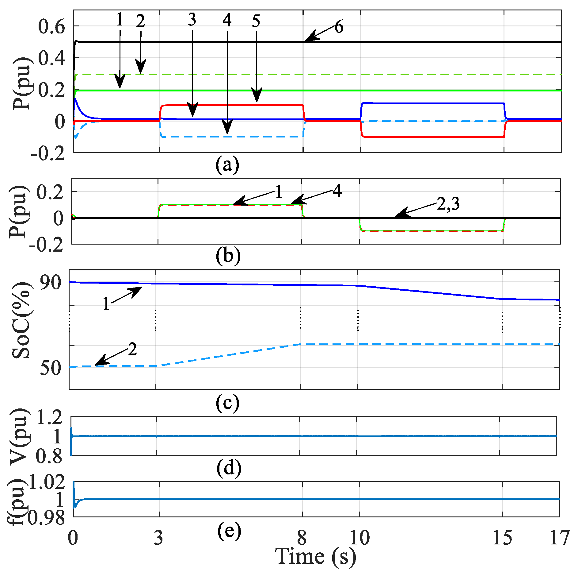
3.5. Central Coordination for Power Contribution

The previous scenarios demonstrate that the proposed controllers are capable of providing a fully seamless operation, controlling voltage and frequency, balancing generation with demand, maintaining practical limitations and riding through faults and sudden changes in load/generation without any central communications. Having said that, the solution is supported by a central control capability to coordinate between the different integrated units if needed. Let us assume that the weather forecast predicts cloudy days that would lower the normal PV generation during the load peak of the next day. In such a case, the network operator may decide to charge the batteries from the grid overnight (when it is cheaper) to be discharged later to compensate for the power shortage on the next day. Alternatively, let us assume that there is excess energy stored in the batteries and the network operator wants to sell it to the grid.

To demonstrate such events, one of the ES units (ES-1) is assumed to be fully charged, while ES-2 is at 50% of its capacity. The events of this scenario are as follows:

Initially, P_pv1 = 0.2 pu, P_pv2 = 0.3 pu, P_L = 0.5 pu and all I_op = 0 (see Figure 2b,c). Thus, P_g1 = P_g2 = P_g3 = P_b1 = P_b2 = 0 pu, and there is no energy exchange between the grid and the MG. At t = 3 s, a central command of I_op = +/−0.1 pu is applied to the control systems of ES-2/MGSC-1 for a 5 s time duration. As a result, ES-2 is charged from the main grid, as shown in Figure 12a,b. Note that ES-1 is already fully charged. At t = 8 s, I_op = 0 for 2 s, stopping the energy exchange process. At t=10 s, the central command of I_op = −/+0.1 pu is applied to the control systems of ES-1/MGSC-1 for a time duration of 5 s. As a result, energy is exported from ES-1 (which was fully charged) to the main grid, while the stored energy in ES-2 remains unchanged. Figure 12c shows the batteries’ SoCs during this process. Figure 12d,e show that the load voltage and frequency are maintained during this process, respectively.

These results demonstrate that the proposed method enables a selective energy exchange between units. This capability is needed for future energy markets, which are based on short-term energy auctions from DERs using technologies such as Blockchain.

4. Conclusions

This paper proposes a new modular configuration and control method to interface buffered MGs. Parallel sets of MGSC-NSC with different I_d-V_d droop control characteristics are proposed to enable sequential power exchange with the grid. The proposed structure enables the future expansion of buffered MGs without the need to replace the entire buffering MGSC-NSC with a larger one. Dead zones are applied to the I_d-V_d droop characteristics of the MGSCs and ES units to enable contribution priorities and flexible operational strategies. The proposed sequential control of the buffering converters increases their lifetime by postponing the operation of the next MGSC-NSC until the full capacity of the previous one is exploited. This also reduces the loss, as it is well-known that converters operate more efficiently at higher loads.

The dead zone implemented in the control units of ES systems enables flexible selectivity for charging/discharging the batteries, irrespective of their capacities and SoCs.

As demonstrated, a seamless MG operation in all operational modes/scenarios is obtained using the proposed structure and control method.

While the primary control enables a communication-free operation, fault ride-through and power smoothing/balancing, it is possible to provide a central control to override the primary controller if a selective exchange of energy between the units is needed. Such capability paves the path towards a short-term auction-based energy market, where all DERs, regardless of their size, can contribute to the market.

Finally, the authors admit that adopting the proposed structure involves some practical limitations, from physical restrictions to additional costs, including any operational and structural constraints applied to any network expansion stage, such as compatibility issues, transient overvoltage problems, reinforcing/resizing some network components to meet new fault levels, etc. However, the proposed method also provides flexibility, security and some savings that can potentially, in the long term, compensate for the additional costs. For example, in addition to reducing inverter losses (using the modular structure), the proposed method reduces some costs associated with network reinforcement (e.g., reactive power compensation) and some operational modes, such as fault ride-through and network reconnection. Nonetheless, a cost–benefit analysis is beyond the scope of this paper.

Several future studies are suggested based on the proposed technique, such as studies on the converter harmonic performance, the network harmonic stability, the associated telephone interference and new filter requirements. In addition, an investigation into combining the proposed design with different HVDC system topologies would be of interest.

PSCAD/EMTDC was used to simulate extensive scenarios in order to prove the superior performance of the proposed design.