Article

Data-Free and Data-Efficient Physics-Informed Neural Network Approaches to Solve the Buckley–Leverett Problem

1
Department of Petroleum Engineering, Khalifa University of Science and Technology, Abu Dhabi 127788, United Arab Emirates
2
College of Information Technology, UAE University, Al Ain 15551, United Arab Emirates
*
Author to whom correspondence should be addressed.
Energies 2022, 15(21), 7864; https://doi.org/10.3390/en15217864
Submission received: 11 September 2022 / Revised: 17 October 2022 / Accepted: 21 October 2022 / Published: 23 October 2022
(This article belongs to the Special Issue Recent Advances in Reservoir Simulation)

Abstract

:
Physics-informed neural networks (PINNs) are an emerging technology in the scientific computing domain. Contrary to data-driven methods, PINNs have been shown to be able to approximate and generalize well a wide range of partial differential equations (PDEs) by imbedding the underlying physical laws describing the PDE. PINNs, however, can struggle with the modeling of hyperbolic conservation laws that develop shocks, and a classic example of this is the Buckley–Leverett problem for fluid flow in porous media. In this work, we explore specialized neural network architectures for modeling the Buckley–Leverett shock front. We present extensions of the standard multilayer perceptron (MLP) that are inspired by the attention mechanism. The attention-based model was, compared to the multilayer perceptron model, and the results show that the attention-based architecture is more robust in solving the hyperbolic Buckley–Leverett problem, more data-efficient, and more accurate. Moreover, by utilizing distance functions, we can obtain truly data-free solutions to the Buckley–Leverett problem. In this approach, the initial and boundary conditions (I/BCs) are imposed in a hard manner as opposed to a soft manner, where labeled data are provided on the I/BCs. This allows us to use a substantially smaller NN to approximate the solution to the PDE.

1. Introduction

The Buckley–Leverett problem is key to understanding many fluid flow processes in porous media. It describes the immiscible and incompressible displacement of a fluid by another in a one-dimensional homogeneous porous media [1]. The generalization of this multiphase flow process is of major interest in many fields such as hydrology and contaminant transport, hydrocarbon recovery, geological CO2 sequestration, etc. At first glance, the problem may appear simple; however, a detailed analysis of the problem and its solution reveals one of the key displacement processes in porous materials, that of piston-like displacement. The piston-like displacement arises from the solution of the Buckley–Leverett problem with a non-convex flux (fractional flow) function, see Figure 1. From a mathematical perspective, solving the PDE associated with Buckley–Leverett, results in an unphysical solution, with two co-existing water saturations at the same point. This unphysical solution is due to the assumption that the water saturation function is continuous and differentiable. In reality, a shock front develops with a discontinuous gradient. As a result, accurately modeling the Buckley–Leverett shock front is known to be challenging using traditional numerical methods (e.g., finite-difference, element, and volume methods).
There are several techniques to solve the Buckley–Leverett problem analytically, such as the Welge [2] graphical method and the Method of Characteristics [3,4,5]. In addition, numerical techniques exist to solve the Buckley–Leverett problem, but these generally result in a diffused shock front due to the truncation error of the numerical approach resembled by the addition of a second-order derivative (diffusion term) to the PDE. As more advanced numerical methods are developed, they are usually benchmarked against the analytical solution of the Buckley–Leverett problem [5,6,7]. PINNs offers an alternative approach to solving partial differential equations via NNs. In this work, we will utilize PINNs for the Buckley–Leverett problem and explore its advantages and disadvantages.
In recent years, machine learning for scientific computing has become a flourishing research domain. This growth has been fueled by the remarkable success of physics-informed neural networks (PINNS) following the seminal 2019 paper by Maziar Raissi et al. [8]. Raissi et al. revived an old idea, using neural networks to solve PDEs by complementing it with modern advances in deep learning, namely, automatic differentiation. In addition, Raissi coined the term physics-informed neural networks (PINNs). Briefly, PINNs are a class of deep-learning algorithms that can seamlessly integrate data and abstract mathematical operators, including PDEs, into neural networks (NN). This novel approach to solve PDEs offers many advantages over traditional-numerical and data-driven approaches [9]. One of the main advantages of PINNs is that it can deal with highly nonlinear PDEs, which conventional methods cannot treat accurately or efficiently [8,9,10,11,12]. PINNs also offer mesh-free solutions as they utilize Automatic Differentiation for computing gradients, avoiding truncation errors associated with traditional numerical techniques [9,13]. In addition, the computational cost of PINNs does not grow exponentially with the number of grid points, which is contrary to traditional numerical methods. Furthermore, the PINNs solution can be evaluated on grids of various resolutions with no extra overhead. Contrary to data-driven approaches, PINNs are data efficient as they only require initial and boundary conditioned data, resulting in considerable gains in efficiency [8,9,10]. Moreover, no prior knowledge of the solution is needed with PINNs, resulting in additional savings on computational resources. PINNs offer a self-contained framework for solving inverse problems with minimal changes in code [8,9,10]. PINNs also promise a robust extrapolation performance, and this is especially important in temporal problems where we would be interested in evaluating future solutions to a dynamical system without extra computational costs.
Despite their great potential, PINNs are still in the early stages of development and are no match for well-developed numerical solvers, as PINNs can be computationally demanding. This is especially true for problems with a large number of collocation points and very deep and wide neural networks. Such cases may require high-memory graphical processing units and/or multiple high-end graphical processing units. Although new and improved NN architectures, improved optimizers, and novel batching algorithms aim to address this problem, it is still an open research question. Furthermore, the relative accuracy of the NN architectures has recently gained notable interest for solving hyperbolic PDEs, specifically the classical Buckley–Leverett problem. Fuks and Tchelipi [14] evaluated PINNs for the solution of the Buckley–Leverett problem in three fluid displacement scenarios: concave, convex, and non-convex flux functions. They identified that PINNs fail in solving the non-convex case. However, the problem was remedied by including an artificial viscosity (second-order derivative) term. This approach resulted in a smoother shock front similar to a numerical solution. Cedric and Tchelipi [15] introduced the Oleinik entropy condition, which acts as an admissibility criterion for propagating shocks. Their solution resulted in a much sharper shock front which precisely mimicked the analytical solution. Diab and Al Kobaisi [16] used the same admissibility criterion and implemented the residual-based adaptive refinement [17] algorithm.
In this study, we investigate the attention-based NN architecture for solving the Buckley–Leverett problem. We note that Rodriguez-Torrado et al. [18] used an attention-based NN architecture to address the Buckley–Leverett problem and arrived at a solution similar to the solution obtained by Fuks and Tchelipi. It is worth noting that Rodriguez-Torrado’s et al. architecture is different from the one evaluated here. In this paper, we implement a new NN architecture that is based on the attention mechanism following Wang et al. [19]. The new NN architecture is used to solve the Buckley–Leverett problem with the Oleinik entropy condition, and the results are compared with the MLP model to gain a broader understanding of the effect of NN architectures.
Another key novelty in this work is solving the Buckley–Leverett problem without any labeled data. In this approach, MLP is utilized, as a mapping between the independent variables and the dependent quantity of interest, while the I/BCs are treated separately in a pre-processing step. This approach alleviates the need for the data-driven term in the loss function and, consequently, the weighing of terms in it. Following the approach proposed by Rao et al. [20], the method entails training two additional low-capacity auxiliary NNs in a preprocessing step. The first NN approximates the distance from any point within the domain to the spatiotemporal boundaries (termed distance network). The second NN approximates the value of the dependent quantity of interest at these boundaries (termed the particular solution network). For relatively simple domain geometries (similar to the one in this work), analytical forms of these two functions exist [21,22,23]. To the best of our knowledge, this is the first implementation of such an approach to the fluid flow in porous media problems.
The paper is organized as follows: in Section 2, we introduce the 1-dimensional incompressible 2-phase flow formulation of the Buckley–Leverett problem along with the necessary boundary conditions. Section 3 presents the mathematical foundation of PINNs. Section 4 presents the multilayer perceptron, the attention-based NN architectures, and the data-free composite NN model. The results are discussed in Section 5. Finally, concluding remarks are given in Section 6. Our code is publicly accessible on GitHub at https://github.com/wandiab/PINNs_BuckleyLeverett (accessed on 28 September 2022) and can be used to reproduce the results herein.

2. Mathematical Formulations

The simulation of 2-phase fluid flow in the porous media is an important problem that commonly arises from the displacement of hydrocarbons by adjacent aquifers and/or in the secondary recovery of oil from subsurface formations. One of the fundamental principles of describing fluid flow in porous media is the Darcy velocity ( v ). In a multi-phase system, the Darcy velocity is defined as follows for each phase α :
v α = K k r α μ α ( p α g ρ α z ) ,  
where K is the permeability tensor, k r α is the relative permeability, μ α is the phase viscosity, p α is the phase pressure, g is the gravitational acceleration, and ρ α is the phase density [24]. The next key principle underpinning fluid flow in the porous medium is the conservation of mass. If we assume that the fluids are incompressible, that is the density is constant, and the porosity only varies in space, then we can assume the flow system to be incompressible. This results in a simplified mass-balance equation in the following form:
S α t + · v α = q α ,  
where S α is the phase saturation and q α is the source/sink term. Using the Darcy velocity (Equation (1)) for a 2-phase oil-water system and noting that S w + S o = 1 we can derive a pressure equation (commonly referred to as the flow equation):
· ( λ K p o ) = q [ λ w p c + ( λ w ρ w + λ o ρ o ) g z ] ,  
where λ is the total mobility defined as λ = λ w + λ o , and p c is the capillary pressure. Furthermore, if we assume p c = 0 , i.e., p w = p o , and a 2D reservoir with no sources/sinks in a homogeneous system ( K = K = c o n s t a n t ), then the flow equation reduces to the following elliptic PDE:
· ( λ K p o ) = 0 .
The saturation equation (commonly referred to as the transport equation) is defined as follows with the same preceding assumptions:
S w t + · ( f w v ) = 0 ,  
where the fractional flow function, f w , is defined as follows:
f w ( S w ) = 1 1 + μ o k r w k r o μ w = S w 2 S w 2 + ( 1 S w ) 2 M   .  
We arrive at this definition for f w by assuming zero initial and residual saturations and using a Brooks–Corey relation for relative permeability; M is the mobility ratio. If we assume = v = 1 , then there is no need to solve a pressure equation, and we retrieve the Buckley–Leverett problem:
S w t + f w = 0 ,     S w ( x , 0 ) = 0 ,     S w ( 0 , t ) = 1 .
Throughout this work, M is taken to be equal to 2 (i.e., oil is twice as viscous as water), resulting in a nonconvex fractional flow function. This type of (nonconvex) fractional flow function (Figure 1) has a characteristic S-shape that results in a discontinuity. It is worth noting that this type of function is the most commonly encountered fractional flow function, and the accurate modeling of such problems is of great interest to porous media research, as evidenced in recent studies [14,15,16]. For instance, Fuks and Tchelipi [14] showed that PINNs struggle to obtain a good solution to the Buckley–Leverett problem with this type of non-convex flux function.
In [15,16], it is shown that an accurate solution using PINNs can be achieved by substituting the nonconvex flux function with a convex hull, as shown in Figure 1 (the red dashed line). The convex hull is a result of using the Oleinik entropy condition (see [4,5]) which is defined as follows:
f ( S ) f ( S l ) S S l σ f ( S ) f ( S r ) S S r ,  
where S l , r are the saturation values just before and after the discontinuity and σ is the shock speed defined as:
σ = f ( S * ) = f ( S * ) S * ,  
where S * is the saturation at the shock-front. The entropy condition acts as an admissibility criterion for propagating discontinuities. For more details on this approach, the reader is referred to the earlier studies [4,5].

3. Physics-Informed Neural Networks (PINNs)

Consider the following differential equation in its most general form:
( u ( 𝓏 ) ) = f ( 𝓏 )                 𝓏   i n   Ω , ( u ( 𝓏 ) ) = g ( 𝓏 )                 𝓏   i n   Ω ,  
where is a non-linear differential operator, u is the unknown solution defined on the domain Ω     d with the boundary Ω , 𝓏 is the space-time coordinate vector ( 𝓏 [ x 1 , ,   x n ; t ] ), and f is the forcing function. The initial condition can be treated as a special type of Dirichlet boundary condition on the spatio-temporal domain, hence, can be denoted as an arbitrary operator and representation of the initial or boundary conditions and g is the boundary function of any type, including Dirichlet, Neumann, Robin, and periodic boundary conditions [9]. In PINNs, the solution u ( 𝓏 ) is approximated via a neural network and parametrized by a set of weights and biases, referred to collectively by θ , as follows:
u ^ θ ( 𝓏 ) u ( 𝓏 ) ,  
where u ^ θ ( 𝓏 ) is the approximated solution by the NN.
The learning process implies the adjustment of NN parameters ( θ ) to satisfy a loss function. The loss function ( ), in principle, consists of two terms: loss on the PDE residual ( ) and loss on the boundary conditions ( ). The residual loss term ( ) is by far the most important term in the loss function as it embeds the physical laws in the NN. Finally, each of the terms is weighed using a parameter ( λ ) to balance the relative importance of each term in the loss function. The loss function has the following form:
( θ ) = λ ( θ ) + λ ( θ ) .  
To find the optimum NN parameters ( θ * ) that satisfy the loss function, the loss function is minimized using a gradient descent algorithm as follows:
θ * = arg min θ   ( λ ( θ ) + λ ( θ ) ) .  
PINNs can be viewed as an unsupervised learning approach as it only utilizes data on the boundary conditions, which is the minimum requirement for a well-posed PDE.
The NN and the loss function are the two main building blocks of PINNs. These two are linked together via automatic differentiation. Automatic differentiation is the feedback mechanism between the loss function and the NN, and it is also the mechanism of computing partial derivatives of the NN to form the PDE residual. In addition, it is the mechanism by which the parameters θ are updated via the gradient descent algorithm. Automatic differentiation capabilities can be leveraged through many of the popular machine-learning packages, such as Tensorflow [25] and PyTorch [26]. The training data are composed of residual points sampled via a Latin hypercube sampling strategy [27], in addition to points randomly sampled on the initial and boundary conditions. In this work, the testing data are 100 × 265 points sampled on a cartesian mesh.

4. Neural Network Architectures

4.1. Multilayer Perceptron Neural NN Architecture

The most common architecture for a deep NN is the multilayer perceptron (MLP), which is a series of linear and nonlinear function transformations applied sequentially to an input ( x ) to produce an output ( u ^ ). The nonlinearity is produced by applying a continuous and differentiable function to the output of each layer, generally referred to as the activation function ( σ ) . The universal approximation theorem provides the mathematical basis for the well-established representational power for NNs [28]. Determining the appropriate NN hyperparameters (i.e., the number of hidden layers and neurons in each layer) to closely approximate a PDE residual can be quite challenging.
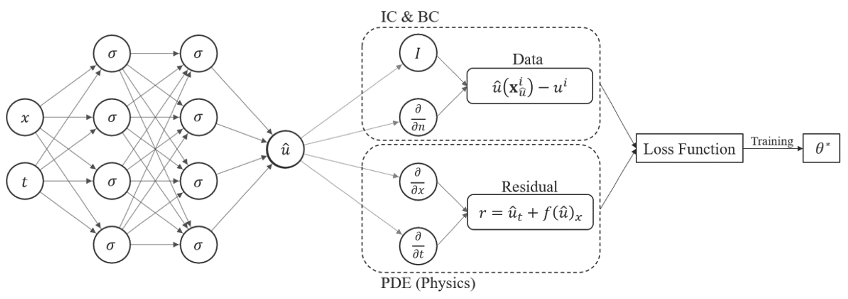
We follow an appealing and mathematically robust definition of MLP—consistent with the recent literature [17]. We identified N L ( x )   :   d i n d o u t to be the ( L 1 ) -hidden layers NN and X = ( x 1 ,   , x d ; t 1 , , t d ) to be the input data containing space and time coordinates, with N neurons in the th layer ( N 0 = d i n ,   N L = d o u t ) . We denoted the weight matrix in the th layer by W N × N 1 , and the bias vector as b N . We referred to the combined set of all weight matrices and bias vectors as θ = { W , b } 1 L . Throughout this work, σ is the hyperbolic tangent (tanh) activation function unless stated otherwise. The MLP architecture is depicted in Figure 2 as part of the PINN framework.
We define the MLP as follows:
input   layer :   N 0 ( X ) = x d i n , hidden   layer :   N ( X ) = σ ( W   N 1 ( X ) + b ) N ,     l = 1 ,     ,   L 1 ,   output   layer :     N L ( X ) = W L   N L 1 ( X ) + b L d o u t

4.2. Attention-Based NN Architecture

In [19], Wang et al. proposed an NN architecture that was inspired by the attention mechanism. The attention mechanism is the building block of transformers, and NN architecture enjoys great success in natural language processing [29]. The proposed architecture was shown to outperform the MLP architecture on a variety of PINNs benchmark problems. Here, we adopt this architecture to solve the Buckley–Leverett problem and benchmark it against the regular MLP for fluid flow in porous media problems.
The forward pass of this architecture is as follows:
U = σ ( X W 1 + b 1 ) ,     V = ( X W 2 + b 2 ) ,   H ( 1 ) = σ ( X W ( l ) + b ( l ) ) ,   Z ( l ) = σ ( H ( k ) W ( l ) + b ( l ) ) ,     l = 1 ,     ,   L 1 ,   H ( l + 1 ) = ( 1 Z ( l ) ) U + Z ( l ) V ,     l = 1 ,     ,   L 1   u θ ( X ) = H ( L ) W ( L ) + b ( L ) ,   θ = { W 1 , b 1 ,   W 2 , b 2 ,   ( W z , l , b z , l ) l = 1 L ,   W , b } .  
The parameters of this architecture are the same as the MLP, and denotes element-wise multiplication. U and V are two transformer networks that project the input variables to a high-dimensional feature space. This is shown in Figure 3 (blue) as part of the PINN framework, where two transformer networks ( U and V ) account for multiplicative interactions between the inputs leading to higher data efficiency and predictive accuracy. This allows the NN to better describe the relationships between the input variables, which in turn, translates to a better predictive performance.

4.3. Data-Free Composite NN Model

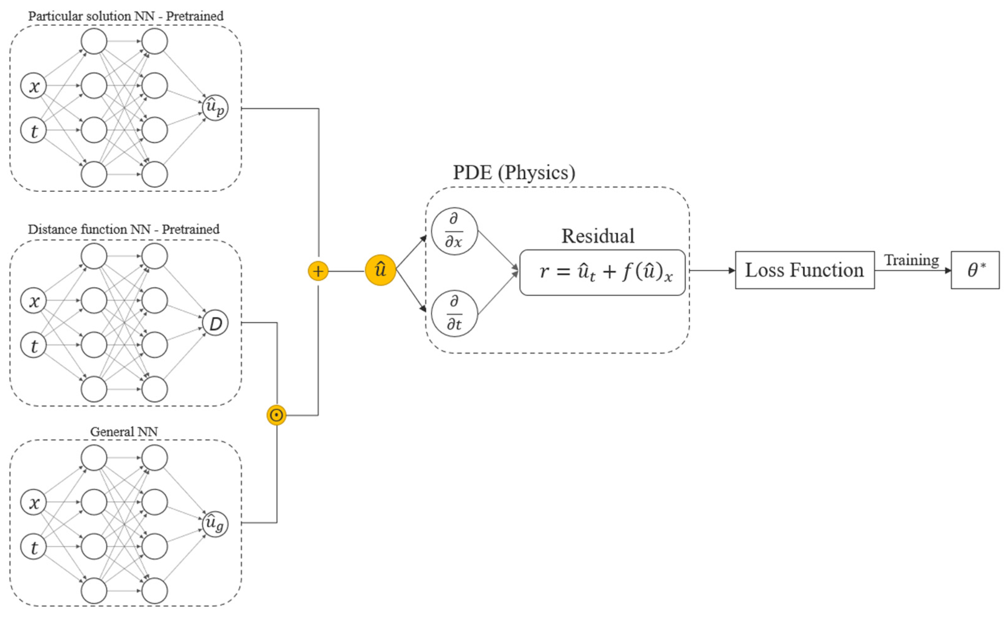
In this section, we introduce a PINNs solution approach to the Buckley–Leverett problem that does not require labeled data. In vanilla PINNs, I/BCs are enforced as a data term in the loss function (Equation (12)). This “soft” enforcement approach can present some difficulty in balancing the different terms in the loss function during training which arises from gradient pathologies [19]. This issue is exacerbated as the number of terms in the loss function grows in 2-D and 3-D domains with multiple types of boundary conditions. Alternatively, the “hard” enforcement of boundary conditions circumvents this problem completely as all terms relating to I/BCs in the loss function are discarded, hence, the name data-free approach. Following Rao et al. [20], the hard enforcement of I/BCs is achieved via a composite scheme that involves three independent NNs. The NNs are termed particular network ( N p ), distance function network ( N D ), and general solution network ( N g ). These three networks are combined in the following manner to achieve a well-posed solution to the Buckley–Leverett PDE:
u ( X ) = N p ( X ; θ p ) + N D ( X ; θ p ) · N g ( X ; θ p ) .  
The first NN ( N p ) represents the actual numerical value at each of the boundary/initial conditions:
u ^ p ( x , t ; θ p ) = { 1 ,       f o r   ( x , t ) Ω D × [ 0 , T ] 0 ,       f o r   ( x , t ) Ω × { t = 0 } ,  
where u ^ p is the output of the particular solution NN. The particular solution network is trained separately in a preprocessing step. The second NN ( N D ) represents the distance between every point in the domain and the spatiotemporal boundaries of the domain. To train the distance function network, we sampled points from a cartesian grid with the dimensionality of the domain and computed the minimum distance between each point and the spatiotemporal boundary as follows:
D ( x , t ) = min ( distance   to   the   spatiotemporal   boundary ) .  
We then passed this grid as inputted to the distance function network, and the network was trained with the labels provided by D ( x , t ) , as defined in Equation (18). As a result, the distance function network predicted the highest values furthest away from a boundary and predicted zero when at a boundary. Similar to the particular solution network, the distance function network was also trained separately in a preprocessing step. The third NN, the general solution network ( N g ), was the only trainable network to satisfy the residual. Its input was a set of collocation points, and its output was the dependent quantity of interest. It is worth mentioning here that each of these three networks should have the same number of input and output units, and only the general solution network weights and biases are trainable by the optimizer once the preprocessing steps are complete.
To summarize, the general solution network on its own is an ill-posed PDE that is then multiplied by the distance function; at the spatiotemporal boundaries of the domain, the product evaluates to zero while the particular solution network evaluates the value of the boundary condition and is summed to fill in for zero product. The result of this operation is a well-posed PDE that is data free since both N p and N d are pre-trained, as shown in Figure 4.

5. Results

In this section, we will first benchmark the attention-based NN architecture against the MLP. Later we will present a completely data-free approach to solve the Buckley–Leverett problem. To quantify the accuracy of PINNs, we compared the results from the two PINNs models with the analytical solution of the Buckley–Leverett problem. We used quantitative and qualitative metrics to quantify the error. Quantitatively, we computed the relative L 2 error for the entire solution. Qualitatively, we took snapshots of the time and plot of the PINNs solution on top of the analytical solution. This allowed us to pick artifacts from the solution since the L 2 reduces everything to a single number.

5.1. Solution of the Buckley–Leverett Problem Using PINNs

We define the residual of the PDE ( r ( x ,   t ; θ ) ) to be the left-hand-side of Equation (7) as follows:
r u ^ t + f ( u ^ ) x ,  
where u ^ is the NN approximation of the saturation function. Using a PINNs approach to solve the Buckley–Leverett problem, we formulated the following loss function:
( θ ; N ) B L = λ r r ( θ ; N r ) + λ u ^ u ^ ( θ ; N u ^ ) ,  
where
u ^ ( θ ; N u ^ ) = 1 N u ^ x N u ^ u ^ ( X u ^ i ) u i 2 2 , r ( θ ; N r ) = 1 N r x N r r ( X r i ) 2 2 .
In Equation (18), u ^ is the loss function on the initial and boundary conditions data, where { x u ^ i , u i }   i = 1 N u ^ are randomly sampled initial and boundary training data, r imposes the residual defined in Equation (16), and { x r i }   i = 1 N r is the set of the interior (collocation) points using a Latin hypercube sampling strategy. Here, we set λ u ^ = λ r = 1 . In the MLP case, the limited-memory Broyden-Fletcher-Goldfarb-Shanno (L-BFGS) [30] optimizer was used, while in the attention-based case, we used the ADAM [31] optimizer.

5.1.1. MLP Model—Buckley–Leverett

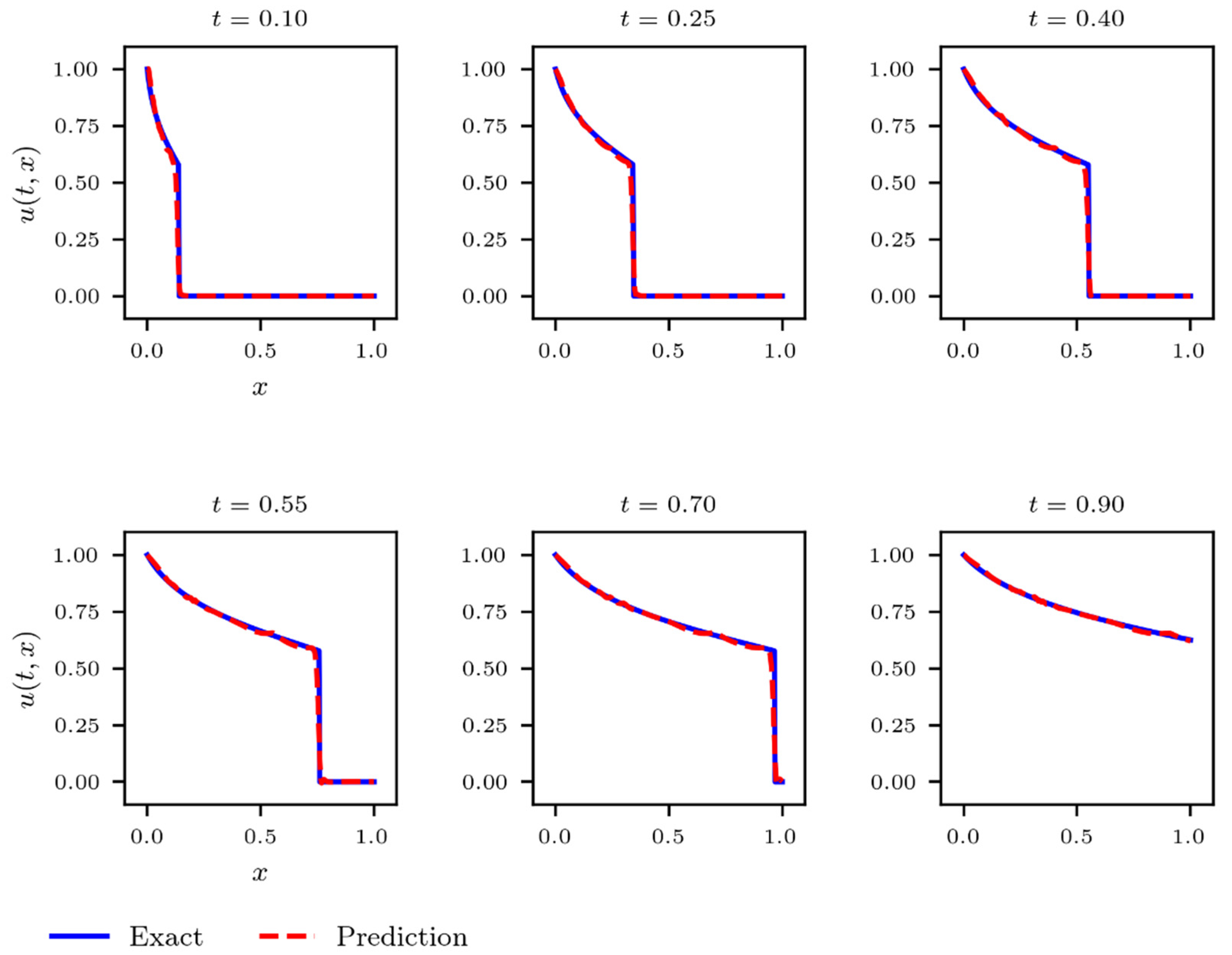
Following our work in [16], we used a deep neural network with eight layers and 20 neurons per layer to solve the Buckley–Leverett problem. In addition, we used 300 points sampled from the initial and boundary condition ( N u ^ = 300 ) and 10,000 collocation points ( N r = 10 , 000 ) sampled from the interior of the domain to solve the Buckley–Leverett problem with an MLP. The resulting L 2 error was 2.81 × 10 2 , and the solution profile is shown in Figure 5. It is clear from Figure 5 that the predicted solution based on the MLP model agrees well with the analytical solution.

5.1.2. Attention-Based Model—Buckley–Leverett

In this section, we will utilize the attention-based NN architecture described in Section 4.2. This architecture utilizes only six layers and 20 neurons per layer to solve the Buckley–Leverett problem and uses the sigmoid activation function for output units; this is undertaken to constrain the output of the network between zero and one, as these are the initial and boundary condition values, respectively. In addition, we achieved a reduction in the number of the sampled points on the initial and boundary conditions from 300 to 250 points and the number of residual points from 10,000 to 2000, all while achieving a lower L 2 error of 1.89 × 10 2 . The solution profile is shown in Figure 5. It is evident from Figure 5 that the attention-based model matched remarkably well with the exact solution. Table 1 shows a comparison between the two architectures.

5.2. Data-Free Composite NN Model Solution of the Buckley–Leverett

The composite scheme presented in this section required the training of three NNs in total, all utilizing the MLP NN architecture described in Section 4.1. The first NN is the particular solution NN which is trained with 5000 points sampled on the initial and boundary conditions for a total of N p = 10,000   points. The particular solution NN consists of four layers and 20 neurons per layer. The hyperbolic tangent (tanh) activation function is used for the hidden layers, and the sigmoid activation function is used for the output layer. We found that restraining the output of the NN with such an approach facilitated the training. The loss function for the particular solution NN ( p ) is as follows:
p ( θ ; N p ) = 1 N p x N p u ^ p ( X u ^ p i ) u p i 2 2 .
The particular solution NN is trained for 1000 iterations using the Adam optimizer with an exponentially decaying learning rate of 1 × 10 2 and then with the L-BFGS optimizer until convergence. The L 2 loss of the particular solution NN is on the order of 1 × 10 14 .
The second NN to be trained is the distance function NN. This network is trained with points sampled on a ( 50 × 50 ) cartesian grid for a total of N D = 2500 . The NN consists of five layers with 20 neurons per layer. The rectified-linear unit (ReLU) activation function is used for all the layers in this network. The loss function for the distance function NN ( D ) is
D ( θ ; N D ) = 1 N D x N D D ^ ( X i ) D ( X i ) 2 2 ,
where D ^ is the output of the distance function NN and D is the distance to the spatiotemporal boundary defined by Equation (18). The training of this NN is conducted in a similar manner to the previous NN. The L 2 loss of the distance function NN is on the order of 1 × 10 8 .
For the general solution network, the loss function defined in Equation (20) reduces to the following as the data term is dropped:
( θ ; N r ) g = r ( θ ; N r ) = 1 N r x N r r ( X r i ) 2 2   .
The general solution network consists of only four layers with 20 neurons per layer, making it by far the most efficient architecture presented in this work. Halving the number of hidden layers means halving the number of trainable parameters. However, the downside is that it requires up to 90,000 collocation points as opposed to only 10,000 points and 2000 points for the MLP and attention-based approaches, respectively; this results in about a 3-fold increase in memory requirement, but fortunately does not translate to a substantial decrease in computational speed. It is worth noting that the hyperparameters of all three networks were manually tuned, and although we are confident in our tuning, there could exist a better combination for these hyperparameters. The general solution network is trained for 150,000 iterations using the Adam optimizer with an exponentially decaying learning rate of 1 × 10 3 .
This data-free composite approach with I/BCs imposed in a hard manner achieved a L 2 error of 4.36 × 10 2 which is slightly higher than the other two methods. The solution profile is shown in Figure 6, and Table 1 gives a comparison between the three architectures.

6. Conclusions and Remarks

Accurately modeling the Buckley–Leverett shock front is known to be challenging using traditional numerical methods (e.g., finite-difference, element, and volume methods). Physics-informed neural networks offer an alternative approach to solve the Buckley–Leverett problem via neural networks. This work presented three distinctive physics-informed neural networks models: (1) the Multilayer perceptron model, (2) the attention-based model, and (3) the data-free composite neural networks model. Our results suggest that the attention-based neural network architecture is better than the multilayer perceptron approach in terms of: (a) data requirements and (b) the accuracy of the two architectures (refer to Table 1). Moreover, the data-free composite neural network model offers a truly data-free approach to solving the Buckley–Leverett problem, albeit being slightly less accurate than the other two models. Tuning the hyperparameters of the data-free composite neural network model could result in higher accuracy and is currently a subject of our ongoing research.
The results of this study provide a comparative evaluation of the neural network architectures and thus add to our overall understanding of the implementation of physics-informed neural networks for fluid flow in porous media problems. The physics-informed neural networks approach may not be mature enough to compete with traditional methods as of yet; however, efforts amongst the scientific computing community to develop physics-informed neural networks into a robust alternative are ongoing.

Author Contributions

Conceptualization, W.D. and M.A.K.; methodology, W.D.; software, W.D., W.Z. and O.C.; validation, W.D., M.A.K. and S.A.; formal analysis, W.D.; investigation, W.D.; data curation, W.D., O.C. and W.Z.; writing—original draft preparation, W.D., M.A. and M.A.K.; writing—review and editing, W.D., M.A.K., M.A. and S.A.; visualization, W.D.; supervision, M.A.K.; project administration, M.A.K. All authors have read and agreed to the published version of the manuscript.

Funding

This research received no external funding.

Data Availability Statement

Not applicable.

Conflicts of Interest

The authors declare no conflict of interest.

References

  1. Dake, L.P. Fundamentals of Reservoir Engineering; Elsevier: Amsterdam, The Netherlands, 1983. [Google Scholar]
  2. Welge, H.J. A Simplified Method for Computing Oil Recovery by Gas or Water Drive. J. Pet. Technol. 1952, 4, 91–98. [Google Scholar] [CrossRef]
  3. Lax, P.D. Hyperbolic Systems of Conservation Laws and the Mathematical Theory of Shock Waves; Society for Industrial and Applied Mathematics: Philadelphia, PA, USA, 1973. [Google Scholar]
  4. LeVeque, R.J. Finite Volume Methods for Hyperbolic Problems; Cambridge University Press: Cambridge, UK, 2002; Volume 31. [Google Scholar]
  5. Lie, K.-A. An Introduction to Reservoir Simulation Using MATLAB/GNU Octave: User Guide for the MATLAB Reservoir Simulation Toolbox (MRST); Cambridge University Press: Cambridge, UK, 2019. [Google Scholar]
  6. Pasquier, S.; Quintard, M.; Davit, Y. Modeling two-phase flow of immiscible fluids in porous media: Buckley-Leverett theory with explicit coupling terms. Phys. Rev. Fluids 2017, 2, 104101. [Google Scholar] [CrossRef] [Green Version]
  7. Abreu, E.; Vieira, J. Computing numerical solutions of the pseudo-parabolic Buckley–Leverett equation with dynamic capillary pressure. Math. Comput. Simul. 2017, 137, 29–48. [Google Scholar] [CrossRef]
  8. Raissi, M.; Perdikaris, P.; Karniadakis, G. Physics-informed neural networks: A deep learning framework for solving forward and inverse problems involving nonlinear partial differential equations. J. Comput. Phys. 2018, 378, 686–707. [Google Scholar] [CrossRef]
  9. Cuomo, S.; Di Cola, V.S.; Giampaolo, F.; Rozza, G.; Raissi, M.; Piccialli, F. Scientific Machine Learning Through Physics–Informed Neural Networks: Where we are and What’s Next. arXiv 2022, arXiv:2201.05624. [Google Scholar] [CrossRef]
  10. Raissi, M.; Karniadakis, G.E. Hidden physics models: Machine learning of nonlinear partial differential equations. J. Comput. Phys. 2018, 357, 125–141. [Google Scholar] [CrossRef] [Green Version]
  11. Zhang, W.; Al Kobaisi, M. On the Monotonicity and Positivity of Physics-Informed Neural Networks for Highly Anisotropic Diffusion Equations. Energies 2022, 15, 6823. [Google Scholar] [CrossRef]
  12. Zhang, W.; Al Kobaisi, M. Cell-Centered Nonlinear Finite-Volume Methods with Improved Robustness. SPE J. 2020, 25, 288–309. [Google Scholar] [CrossRef]
  13. Jin, X.; Cai, S.; Li, H.; Karniadakis, G.E. NSFnets (Navier-Stokes flow nets): Physics-informed neural networks for the incompressible Navier-Stokes equations. J. Comput. Phys. 2020, 426, 109951. [Google Scholar] [CrossRef]
  14. Fuks, O.; Tchelepi, H.A. Limitations Of Physics Informed Machine Learning For Nonlinear Two-Phase Transport In Porous Media. J. Mach. Learn. Model. Comput. 2020, 1, 19–37. [Google Scholar] [CrossRef]
  15. Fraces, C.G.; Tchelepi, H.; Hamdi, T. Physics informed deep learning for flow and transport in porous media. In SPE Reservoir Simulation Conference; OnePetro: Richardson, TX, USA, 2021. [Google Scholar]
  16. Diab, W.; Kobaisi, M.A. PINNs for the Solution of the Hyperbolic Buckley-Leverett Problem with a Non-convex Flux Function. arXiv 2021, arXiv:2112.14826. [Google Scholar]
  17. Lu, L.; Meng, X.; Mao, Z.; Karniadakis, G.E. DeepXDE: A Deep Learning Library for Solving Differential Equations. SIAM Rev. 2021, 63, 208–228. [Google Scholar] [CrossRef]
  18. Rodriguez-Torrado, R.; Ruiz, P.; Cueto-Felgueroso, L.; Green, C.M.; Friesen, T.; Matringe, S.; Togelius, J. Physics-informed attention-based neural network for solving non-linear partial differential equations. arXiv 2021, arXiv:2105.07898. [Google Scholar]
  19. Wang, S.; Teng, Y.; Perdikaris, P. Understanding and Mitigating Gradient Flow Pathologies in Physics-Informed Neural Networks. SIAM J. Sci. Comput. 2021, 43, A3055–A3081. [Google Scholar] [CrossRef]
  20. Rao, C.; Sun, H.; Liu, Y. Physics-Informed Deep Learning for Computational Elastodynamics without Labeled Data. J. Eng. Mech. 2021, 147, 04021043. [Google Scholar] [CrossRef]
  21. Sun, L.; Gao, H.; Pan, S.; Wang, J.-X. Surrogate modeling for fluid flows based on physics-constrained deep learning without simulation data. Comput. Methods Appl. Mech. Eng. 2019, 361, 112732. [Google Scholar] [CrossRef] [Green Version]
  22. Samaniego, E.; Anitescu, C.; Goswami, S.; Nguyen-Thanh, V.M.; Guo, H.; Hamdia, K.; Zhuang, X.; Rabczuk, T. An energy approach to the solution of partial differential equations in computational mechanics via machine learning: Concepts, implementation and applications. Comput. Methods Appl. Mech. Eng. 2020, 362, 112790. [Google Scholar] [CrossRef] [Green Version]
  23. Dong, S.; Ni, N. A method for representing periodic functions and enforcing exactly periodic boundary conditions with deep neural networks. J. Comput. Phys. 2021, 435, 110242. [Google Scholar] [CrossRef]
  24. Muskat, M. The Flow of Homogeneous Fluids Through Porous Media. Soil Sci. 1938, 46, 169. [Google Scholar] [CrossRef]
  25. Abadi, M.; Barham, P.; Chen, J.; Chen, Z.; Davis, A.; Dean, J.; Devin, M.; Ghemawat, S.; Irving, G.; Isard, M.; et al. {TensorFlow}: A system for {Large-Scale} machine learning. In Proceedings of the 12th USENIX Symposium on Operating Systems Design and Implementation (OSDI 16), Savannah, GA, USA, 2–4 November 2016; pp. 265–283. [Google Scholar]
  26. Paszke, A.; Gross, S.; Massa, F.; Lerer, A.; Bradbury, J.; Chanan, G.; Killeen, T.; Lin, Z.; Gimelshein, N.; Antiga, L.; et al. Pytorch: An imperative style, high-performance deep learning library. In Proceedings of the Advances in Neural Information Processing Systems 32 (NeurIPS 2019), Vancouver, BC, Canada, 8–14 December 2019; Volume 32. [Google Scholar]
  27. McKay, M.D.; Beckman, R.J.; Conover, W.J. A comparison of three methods for selecting values of input variables in the analysis of output from a computer code. Technometrics 2000, 42, 55–61. [Google Scholar] [CrossRef]
  28. Hornik, K.; Stinchcombe, M.; White, H. Multilayer feedforward networks are universal approximators. Neural Netw. 1989, 2, 359–366. [Google Scholar] [CrossRef]
  29. Vaswani, A.; Shazeer, N.; Parmar, N.; Uszkoreit, J.; Jones, L.; Gomez, A.N.; Kaiser, Ł.; Polosukhin, I. Attention is all you need. In Proceedings of the Advances in Neural Information Processing Systems 30 (NIPS 2017), Long Beach, CA, USA, 4–9 December 2017; Volume 30. [Google Scholar]
  30. Zhu, C.; Byrd, R.H.; Lu, P.; Nocedal, J. Algorithm 778: L-BFGS-B: Fortran subroutines for large-scale bound-constrained optimization. ACM Trans. Math. Softw. (TOMS) 1997, 23, 550–560. [Google Scholar] [CrossRef]
  31. Kingma, D.P.; Ba, J. Adam: A method for stochastic optimization. arXiv 2014, arXiv:1412.6980. [Google Scholar]
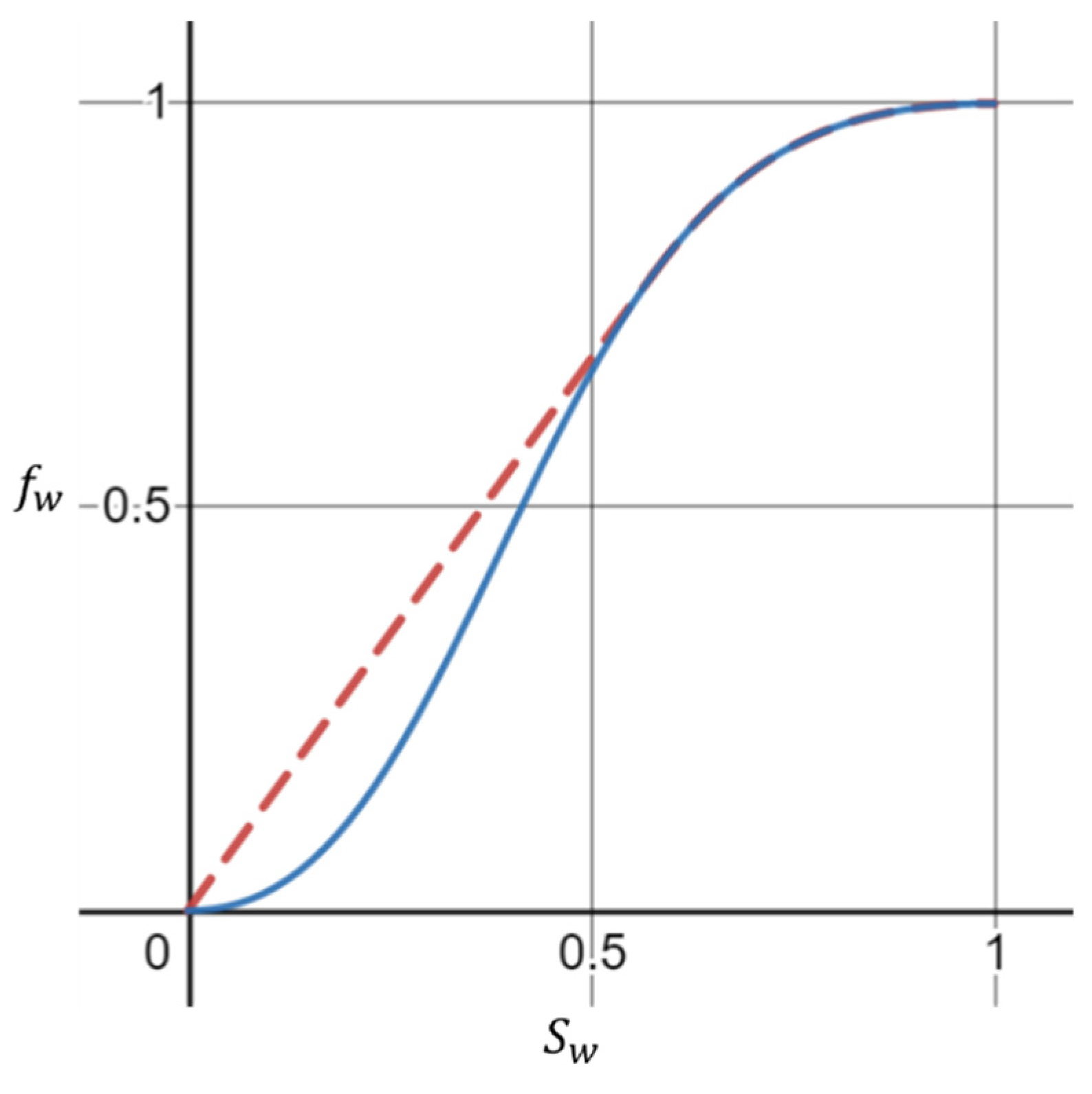
Figure 1. Nonconvex fractional flow function (blue) with an Oleinik entropy condition concave envelope (dashed red).
Energies 15 07864 g001
Figure 2. A representative PINN architecture for the solution of the hyperbolic Buckley–Leverett problem.
Energies 15 07864 g002
Figure 3. A representative PINN architecture for the solution of the hyperbolic Buckley–Leverett problem. In black is the MLP architecture. In blue is the input encoding of the attention mechanism.
Energies 15 07864 g003
Figure 4. Data-free composite PINN architecture for the solution of the hyperbolic Buckley–Leverett problem. Note: the backbone of the model could be an MLP or an attention model and the I/BCs are enforced in a hard manner.
Energies 15 07864 g004
Figure 5. Comparison between PINNs solutions, MLP and attention-based, (dashed line) and the analytical solution (solid line) at six different times.
Energies 15 07864 g005
Figure 6. Comparison between composite data-free PINNs solution (dashed line) and the analytical solution (solid line) at six different times.
Energies 15 07864 g006
Table 1. Comparison between the MLP and the attention-based architectures.
# of Layers N r N u ^ L 2 Error
MLP 810,000300 2.81 × 10 2
Attention 62000250 1.89 × 10 2
Data-free 490,0000 4.36 × 10 2
Publisher’s Note: MDPI stays neutral with regard to jurisdictional claims in published maps and institutional affiliations.