Abstract
This work reviews from a unified viewpoint the concepts underlying the “nth-Order Comprehensive Adjoint Sensitivity Analysis Methodology for Response-Coupled Forward/Adjoint Linear Systems” (nth-CASAM-L) and the “nth-Order Comprehensive Adjoint Sensitivity Analysis Methodology for Nonlinear Systems” (nth-CASAM-N) methodologies. The practical application of the nth-CASAM-L methodology is illustrated for an OECD/NEA reactor physics benchmark, while the practical application of the nth-CASAM-N methodology is illustrated for a nonlinear model of reactor dynamics that exhibits periodic and chaotic oscillations. As illustrated both by the general theory and by the examples reviewed in this work, both the nth-CASAM-L and nth-CASAM-N methodologies overcome the curse of dimensionality in sensitivity analysis. The availability of efficiently and exactly computed sensitivities of arbitrarily high order can lead to major advances in all areas that need such high-order sensitivities, including data assimilation, model calibration, uncertainty reduction, and predictive modeling.
1. Introduction
The computational model of a physical system comprises the following fundamental conceptual components: (a) a well-posed system of equations that relate the system’s independent variables and parameters to the system’s state (i.e., dependent variables); (b) nominal or mean values for the system parameters, along with information regarding the probability distributions, moments thereof, and inequality and/or equality constraints that define the range of variations in the system’s parameters; and (c) one or several quantities, customarily referred to as model/system responses (or objective functions, or indices of performance), which are computed using the mathematical model. The functional derivatives of model responses with respect to model parameters are called “sensitivities” (of responses with respect to model parameters). The computation of higher-order sensitivities by conventional methods is subject to the “curse of dimensionality”, a term coined by Belmann [1] to describe phenomena in which the number of computations increases exponentially in the respective phase space. In the particular case of sensitivity analysis, the number of large-scale computations increases exponentially in the parameter phase space as the order of sensitivities increases if conventional methods (e.g., finite differences) are used: thus, if a model has TP parameters, the computation of first-order sensitivities requires at least 2TP large-scale computations; the computation of second-order sensitivities requires at least (3TP)2 computations, and so on; and the computation of the nth-order sensitivities requires at least (nTP)n large-scale computations.
A fundamental breakthrough in the sensitivity analysis of problems of interest to nuclear reactor physics, which are governed by the linear Boltzmann transport equation, was achieved by Wigner [2], who pioneered the use of the adjoint Boltzmann transport equation to compute first-order perturbations (and, hence, first-order sensitivities) in the reactor’s multiplication factor arising from perturbations in the model parameters (nuclear cross sections). Wigner’s method became widespread in the nuclear engineering community and was considered to be adequate for predicting the effects of small parameter changes on the model responses, as well as for performing [3,4] a first-order uncertainty quantification of the standard deviation induced in a model response due to uncertainties (standard deviations and correlations) affecting the model parameters (nuclear cross sections). This situation changed after Goldstein [5] reported studies of neutron transmission through a sodium shield, which showed that even for modest variations of 5% in the cross section at the 297 keV sodium minimum, the first-order sensitivities of responses measured by detectors differed by 20–50% from their correct/actual values. These results indicated that the nonlinear dependence of a detector’s response on the sodium cross section in deep-penetration radiation and neutron shielding problems cannot be predicted by first-order sensitivities, despite the fact that the physics of neutron/gamma transport through materials is governed by the linear Boltzmann equation. These findings have motivated Greenspan et al. [6] to propose an extension of Wigner’s method [2], so as to enable the computation of second-order sensitivities of detector responses to neutron cross sections for linear neutron transport problems. Greenspan et al. [6] concluded that their methodology “appears to provide satisfactory accuracies for most non-linear problems associated with cross section changes encountered in practice”. This conclusion, while correct for the particular “neutron-transmission through a sodium shield problem” under investigation, is actually incorrect in general since, as is shown in the remainder of this work, third- and fourth-order sensitivities of responses with respect to cross sections are even more important than the second-order sensitivities in reactor physics problems. Greenspan et al. [6] further stated that: “The use of higher (than second) order sensitivity theories like the one recently proposed by Gandini [7]—is not likely to be desirable—the added accuracy provided, say, by a third order formulation is not likely to justify the additional computational effort required for its application”. Again, this statement by Greenspan et al. [6] is correct regarding the methodology proposed by Gandini [7], which is not only cumbersome and computationally inefficient but is also limited to formal time-dependent linear neutron transport and/or diffusion problems. However, the sweepingly general statement by Greenspan et al. [6] that the “use of higher (than second) order sensitivity theories…is not likely to be desirable” is proven to be incorrect in the remainder of this work by showing that the third- and fourth-order sensitivities of responses with respect to cross sections are even more important than the second-order sensitivities in reactor physics problems.
Wigner’s methodology and its extensions by Greenspan et al. [6] and Gandini [7] were developed within the specific context of the linear neutron transport equation and are not applicable to nonlinear models, since nonlinear operators do not admit adjoint operators. The rigorous first-order adjoint sensitivity analysis methodology for generic large-scale nonlinear (as opposed to linearized) systems involving generic operator responses has been conceived and developed by Cacuci [8,9], who is also credited (see, e.g., [10,11]) for having introduced these principles to the earth, atmospheric, and other sciences. Cacuci’s [8,9] first-order adjoint sensitivity analysis methodology for nonlinear systems is just as efficient for computing first-order sensitivities as Wigner’s method is for linear systems, requiring a single large-scale (adjoint) computation for obtaining all of the first-order sensitivities, regardless of the number of model parameters. This is in contradistinction with the number of (at least) “2P computations” which would be required by conventional methods (e.g., finite differences). Thus, the methodologies of Wigner [2] and Cacuci [8,9] provided the “first-order cracking of the curse of dimensionality” in sensitivity and uncertainty analysis. Cacuci’s methodology [8,9] has been applied to many (too numerous to cite here) research fields since its publication. Second-order deterministic analyses of specific problems in diverse fields, e.g., structural analysis [12,13], mechanical system [14], atmospheric science [15], linear circuit analysis, and optimization [16], have also been published. General methodologies for the efficient and exact computation of second-order response sensitivities to model responses were proposed by Cacuci for response-coupled forward and adjoint linear systems [17] and for nonlinear systems [18].
The unparalleled efficiency of the second-order adjoint sensitivity analysis methodology for linear systems conceived by Cacuci [17] was demonstrated in [19,20,21,22,23,24] by applying this methodology to compute exactly the 21,976 first-order sensitivities and 482,944,576 s-order sensitivities for an OECD/NEA reactor physics benchmark [25], which is representative of a large-scale system that involves many parameters. The results obtained in [19,20,21,22,23,24] indicated that many second-order sensitivities were much larger than the largest first-order ones, which implies that the consideration of only the first-order sensitivities is insufficient for making credible predictions regarding the expected values and uncertainties (variances, covariances, skewness) of calculated and predicted/adjusted responses. At the very least, the second-order sensitivities must also be computed in order to enable the quantitative assessment of their impact on the predicted model responses.
The findings reported in [19,20,21,22,23,24] motivated the investigation [26,27] of the largest third-order sensitivities, many of which were found to be even larger than the second-order ones. This finding, in turn, has motivated the development [28] of the mathematical framework for determining and computing the fourth-order sensitivities for the OECD/NEA benchmark, many of which were found [29,30] to be larger than the third-order ones. The need for computing the third- and fourth-order sensitivities has been underscored in [31,32]. The efficiency of Cacuci’s new methodology for computing exactly third-order and fourth-order sensitivities while overcoming the curse of dimensionality has been highlighted in [33,34,35].
This sequence of findings has motivated the conception by Cacuci [36] of the “nth-Order Comprehensive Adjoint Sensitivity Analysis Methodology for Response-Coupled Forward/Adjoint Linear Systems” (abbreviated as “nth-CASAM-L”). The nth-CASAM-L enables the efficient computation of exactly determined expressions of arbitrarily high-order sensitivities of a generic system response—which can depend on both the forward and adjoint state functions− with respect to all of the parameters that characterize the physical system. The qualifier “comprehensive” is employed in order to highlight that the model parameters considered within the framework of the nth-CASAM-L include the system’s uncertain boundaries and internal interfaces in the phase space. The nth-CASAM-L mathematical framework was developed specifically for linear systems because the most important model responses produced by such systems are various Lagrangian functionals, which depend simultaneously on both the forward and adjoint state functions governing the respective linear system. Included among such functionals are the Raleigh quotient for computing eigenvalues and/or separation constants when solving linear partial differential equations, and the Schwinger and Rousopoulos functionals (see, e.g., [37,38,39]), which play fundamental roles in optimization and control procedures, derivation of numerical methods for solving equations (differential, integral, integro-differential), and sensitivity analysis. Responses that depend on both the forward and adjoint state functions underlying the respective model can occur only for linear systems, because responses in nonlinear systems can only depend on the system’s forward state functions (since nonlinear operators do not admit adjoint operators). Consequently, the sensitivity analysis of responses that simultaneously involve both forward and adjoint state functions makes it necessary to treat linear models/systems in their own right, rather than treating them as particular cases of nonlinear systems. The nth-CASAM-L is formulated in linearly increasing higher-dimensional Hilbert spaces (as opposed to exponentially increasing parameter-dimensional spaces), thus overcoming the curse of dimensionality in enabling the most efficient computation of exactly determined expressions of arbitrarily high-order sensitivities of generic nonlinear system responses with respect to model parameters, uncertain boundaries, and internal interfaces in the model’s phase space.
In parallel with the aforementioned developments, Cacuci [40,41] has extended his original work [8,9] on nonlinear systems, providing the mathematical framework for deriving and computing efficiently the exact expressions of sensitivities with respect to imprecisely known (i.e., uncertain) model parameters, model boundaries, and/or internal interfaces, up to and including fifth order. Subsequently, Cacuci [42] has generalized the 5th-CASAM-N methodology [41] to enable the exact and efficient computation of sensitivities of arbitrarily high order with respect to model parameters, uncertain boundaries, and internal interfaces in the model’s phase space. This novel general methodology [42], called the nth-Order Comprehensive Adjoint Sensitivity Analysis Methodology for Nonlinear Systems (nth-CASAM-N), is also formulated (just like the nth-CASAM-L) in linearly increasing higher-dimensional Hilbert spaces (as opposed to exponentially increasing parameter-dimensional spaces), thus overcoming the curse of dimensionality in sensitivity analysis of nonlinear systems.
This work is structured as follows: Section 2 highlights the fundamental role of sensitivities in defining the correlations between responses and parameters. If the negative impact of the curse of dimensionality is not alleviated when computing sensitivities, this negative impact is transmitted to the computation of the aforementioned correlations. Section 3.1 illustrates the need for computing high-order sensitivities by reviewing the results obtained in [16,17,18,19,20,21,22,23,24,25,26,27,28,29,30] for an OECD/NEA reactor physics benchmark [25], which is representative of linear models/systems. These results underscore the efficiency of the nth-CASAM-L in overcoming the curse of dimensionality while producing the respective results. Section 3.2 reviews the general mathematical framework underlying the nth-CASAM-L [36].
Section 4.1 reviews the pioneering sensitivity and uncertainty analysis results presented in [43,44] for the reduced-order model developed by March-Leuba, Cacuci, and Perez [45] for studying the nonlinear dynamics displayed by boiling water reactors (BWR). This reduced-order model comprises point neutron kinetics equations coupled nonlinearly to thermal-hydraulics equations that describe the time evolution of the fuel temperature and coolant density in the recirculation loop, which is treated as a single path of fluid of variable cross-sectional area but with constant mass flow, with the coolant entering the core at saturation temperature. This model shows that the major state variables, including power, reactivity, void fraction, and temperature, undergo limit cycle oscillations under high-power/low-flow operating conditions, and the amplitudes of these oscillations are very sensitive to the reactor’s operating conditions. When increasing the heat transfer from the reactor to the coolant, this model indicates that these limit cycle oscillations can become unstable, undergoing period-doubling bifurcations in the time evolutions of the state variables (power, delayed neutron precursors, reactivity, coolant void fraction, fuel temperature) from periodic to aperiodic (chaotic) oscillations. Thus, this nonlinear model [45] illustrates generically the most extreme forms of nonlinear phenomena (from limit cycles to chaos) that can be displayed by nonlinear physical systems. The results of the sensitivity and uncertainty analyses presented in Section 4.1 are obtained by applying the first-order particularization of the nth-CASAM-N [42], the general form of which is reviewed in Section 4.2. The work of March-Leuba, Cacuci, and Perez [45] has inspired several related models of BWR-dynamics [46,47,48,49,50,51,52,53,54,55].
Section 5 reviews the concepts underlying the nth-CASAM-L [36,56] and nth-CASAM-N [42] methodologies from a unified viewpoint, indicating under which circumstances the nth-CASAM-L could be viewed as a particular case of the nth-CASAM-N methodology. As the paradigm examples presented in Section 3.1 and Section 4.1 illustrate, using finite differences for computing high-order sensitivities of model responses to model parameters becomes not only computationally unfeasible for large-scale systems (because of the curse of dimensionality), but finding the optimal step size to minimize the error between the finite difference result and the exact result is practically impossible to achieve unless one knows beforehand what the exact result is—which would be possible only by using the CASAM-L and/or nth-CASAM-N methodologies.
2. The Fundamental Role of High-Order Sensitivities in Defining Correlations among Model Responses and Parameters
The mathematical model of a physical system comprises independent variables (e.g., space, time, etc.), dependent variables (aka “state functions”; e.g., temperature, mass, momentum, etc.), and various parameters (appearing in correlations, coordinates of physical boundaries, etc.), which are all interrelated by equations that usually represent conservation laws. Without loss of generality, the model parameters can be considered to be real scalar quantities, having known nominal (or mean) values and, possibly, known higher-order moments or cumulants (i.e., variance/covariances, skewness, kurtosis), which are usually determined from experimental data and/or processes external to the physical system under consideration. The model parameters usually stem from processes that are external to the system under consideration and are seldom, if ever, known precisely. These imprecisely known model parameters are denoted as ,…, , where the subscript “TP” indicates “Total (number of) Parameters”. It is convenient to consider that these parameters are components of a “vector of parameters”, denoted as , where denotes the TP-dimensional subset of the set of real scalars. These model parameters are considered to include imprecisely known geometrical parameters that characterize the physical system’s boundaries in the phase space of the model’s independent variables. Thus, is a TP-dimensional column vector and its components are considered to include all of the uncertain model parameters, including those that may enter into defining the system’s boundary in the phase space of independent variables. For subsequent developments, it is convenient to denote matrices and vectors using capital and lower case bold letters, respectively. The symbol “” will be used to denote “is defined as” or “is by definition equal to”. Transposition will be indicated by a dagger superscript.
The result of interest computing using a mathematical/computational model of a physical system is, in principle, an implicit function of the system’s parameters . In practice, the model parameters are not known exactly, even though they are not bona fide random quantities. For practical purposes, however, these model parameters are considered to be variates that obey a multivariate probability distribution function, denoted as , which is seldom known, particularly for large-scale systems involving many parameters. Considering that the multivariate distribution is formally defined on a domain , the various moments of can be formally defined in a standard manner by using the following notation
where is a continuous function of the parameters . Thus, the moments of are defined as follows:
- The expected (or mean) value of a model parameter , denoted as , is defined as follows:The expected values are considered to be the components of the following vector of mean (expected) values:
- The covariance, , of two parameters, and , is defined as follows:The variance, , of a parameter , is defined as follows:The standard deviation of a parameter , which is denoted , is defined as follows: . The correlation, , between two parameters and , is defined as follows:
- The third-order correlation, , among three parameters , and , is defined as follows:
- The fourth-order correlation among four parameters, is defined as follows, for :In the important particular case when the parameters are normally distributed, the following relation holds:
The higher-order correlations among parameters are defined following the same pattern as displayed in Equations (6)–(8). In practice, the parameter correlations are estimated using experimental information about the parameters.
The result of interest computed using the model of the physical system under consideration is customarily called a system/model “response” and is denoted as . Being an implicit function of the system’s parameters, the response is considered to admit a formal Taylor series of around a point , which is usually taken to be the vector of expected (or nominal) parameter values, having the following well-known formal expression:
The radius/domain of convergence of the series in Equation (10) must be established before using it for any practical application. The functional derivatives of the model response with respect to the model’s parameters are customarily called the “sensitivities” (of various orders) of the model’s response with respect to the parameters. As is well known, and as indicated by Equation (10), the Taylor series of a function of variables (e.g., ) comprises first-order derivatives, distinct second-order derivatives, distinct third-order derivatives, and so on. The computation by conventional methods of the -order sensitivities of a response with respect to the parameters would require at least large-scale computations. This exponential increase—with the order of response sensitivities—in the number of large-scale computations needed to determine higher-order sensitivities is the manifestation of the “curse of dimensionality in sensitivity analysis”, by analogy to expression coined by Belmann [1] to express the difficulty of using “brute-force” grid search when optimizing a function with many input variables.
It follows from the Taylor series expansion presented in Equation (10) that, in principle, the response and parameters are correlated quantities. The correlations of various orders between a model’s response(s) and parameters are defined as follows.
- The expectation (value), , of a response is defined as follows:
- The covariance between two responses and is defined as follows:
- The triple correlations (or third-order moment of the distribution of responses), denoted as , among three responses , , and , are defined as follows:
- The quadruple correlations (or fourth-order moment of the distribution of responses), denoted as , among four responses , , , and , are defined as follows:
Expressions for the response moments defined in Equations (11)−(14) were first obtained by Tuckey [57], who provided expressions up to fifth order in the parameter standard deviations. Cacuci [56] has generalized Tuckey’s work, providing corresponding expressions up to and including the sixth-order terms in parameter standard deviations. Cacuci [56] has also noticed that the existence of the Taylor-series shown in Equation (10) implies not only correlations among model responses but also correlations among model responses and model parameters, as defined below in Equations (15)−(20), and has provided the corresponding expressions up to and including the sixth-order terms in parameter standard deviations.
- e.
- The covariance between computed responses and a parameter is defined as follows:
- f.
- The triple-correlations among one parameter, , and two responses, and , are defined as follows:
- g.
- The triple correlations among two parameters , and one response are defined as follows:
- h.
- The quadruple correlations denoted as , among one parameter, , and three responses , , and , are defined as follows:
- i.
- The quadruple correlations, denoted as , among two parameters , and two responses , , are defined as follows:
- j.
- The quadruple correlations, denoted as , among three parameters , , and one response, , are defined as follows:
3. High-Order Sensitivity and Uncertainty Analysis of Linear Models/Systems: Illustrative Example and General Theory
Section 3.1 illustrates the need for computing high-order sensitivities by reviewing the results obtained in [16,17,18,19,20,21,22,23,24,25,26,27,28,29,30] for an OECD/NEA reactor physics benchmark [25], comprising a subcritical polyethylene-reflected plutonium metal sphere, which is called the “PERP” (polyethylene-reflected plutonium) benchmark. The PERP benchmark is modeled by using the deterministic neutron transport Boltzmann equation, which is solved numerically (after discretization in the energy, spatial, and angular independent variables) using the software package PARTISN [58]. The numerical model of the PERP benchmark comprises 21,976 uncertain parameters, as follows: 180 group-averaged total microscopic cross sections, 21,600 group-averaged scattering microscopic cross sections, 120 fission process parameters, 60 fission spectrum parameters, 10 parameters describing the experiment’s nuclear sources, and 6 isotopic number densities. In view of the fact that the PERP benchmark is modeled by the integro-differential Boltzmann equation in six independent variables (the solving of which is representative of “large-scale” computations), and since this model involves 21,976 uncertain parameters (which are representative of “many parameters”), the PERP benchmark can be considered to be representative of linear models/systems for the purpose of computing high-order sensitivities.
The results reviewed in Section 3.1 were obtained by applying the nth-CASAM-L, for n = 1, 2, 3, 4, underscoring the efficiency of the nth-CASAM-L in overcoming the curse of dimensionality while producing the respective results. Section 3.2 reviews the general mathematical framework underlying the nth-CASAM-L [36].
3.1. Illustrating the Need for High-Order Sensitivity Analysis and Uncertainty Quantification: A Paradigm Reactor Physics Benchmark
The PERP benchmark is a spherical subcritical nuclear system driven by a source of spontaneous fission neutrons. The PERP benchmark comprises an inner sphere (designated as “material 1” and assigned to “zone 1”) which is surrounded by a spherical shell (designated as “material 2” and assigned to “zone 2”). The inner sphere of the PERP benchmark contains α-phase plutonium which acts as the source of particles; the radius is = 3.794 cm. This inner sphere is surrounded by a spherical shell reflector made of polyethylene with a thickness of 3.81 cm; the radius of the outer shell containing polyethylene is = 7.604 cm. Table 1 specifies the constitutive materials of the PERP benchmark.

Table 1.
Dimensions and composition of the PERP benchmark.
The neutron flux distribution within the PERP benchmark has been computed by using the deterministic software package PARTISN [58], which solves the following multigroup approximation of the transport equation for the group fluxes, :
where:
The PARTISN [58] computations used the SOURCE4C code [59] and the MENDF71X library [60] which comprise 618 group cross sections. These cross sections were collapsed to energy groups, with group boundaries, , as indicated in Figure 1. The MENDF71X library [60] uses ENDF/B-VII.1 nuclear data [61]. The group boundaries, , are user-defined and are therefore considered to be perfectly well-known parameters.
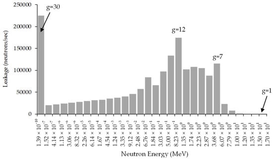
Figure 1.
Histogram plot of the leakage for each energy group for the PERP benchmark.
The fundamental quantities of interest (i.e., “system responses”) for subcritical benchmarks (such as the PERP benchmark) are single-counting rates, double-counting rates, the leakage multiplication, and the total leakage. The total leakage from the outer surface of the PERP sphere was considered to be the paradigm response of interest for illustrating the need for high-order sensitivity analysis, because the total leakage does not depend on the detector configuration (as opposed to count rates) and is therefore more meaningful physically than the count rates.
The total neutron leakage from the PERP sphere, denoted as , depends implicitly (through the neutron flux) on all model parameters and is defined as follows:
The numerical value of the PERP’s benchmark total leakage, computed by using Equation (26), is neutrons/sec. Figure 1 depicts the histogram plot of the leakage for each energy group for the PERP benchmark.
3.1.1. Overview of Results for the First, Second, Third, and Fourth-Order Sensitivities
The computations of the sensitivities, of all orders, were performed deliberately using a widely accessible desktop computer, namely a DELL AMD FX-8350 with an 8-core processor. A single adjoint (large-scale) computation is needed in order to obtain all 21,976 sensitives of the first-level adjoint function, which is subsequently used to compute all of the first-order sensitivities using inexpensive quadrature formulas. The CPU time for a typical PARTISN forward neutron transport computation with an angular quadrature of S32 is ca. 45 s. On the other hand, the CPU time for a typical adjoint neutron transport computation using the neutron transport solver PARTISN with an angular quadrature of S32 is ca. 24 s. The CPU time for computing the integrals over the adjoint function is ca. 0.004 s.
Thus, the exact computation of the 21,976 first-order sensitivities using the first-level adjoint function is (24 + 21,976 × 0.004) s = 112 s. By comparison, the approximate computation of the 21,976 first-order sensitivities using a two-point finite difference formula would require 21,976 × 2 × 45 s = 550 h. Most of the first-order relative sensitivities have been found to be negligibly small, having absolute values less than 0.1. The most important (i.e., largest) sensitivities of the leakage response are with respect to the group-averaged total microscopic cross sections, followed by the sensitivities of the leakage response with respect to the isotopic number densities. Only 16 first-order relative sensitivities have absolute values greater than 1.0; most of these involve the total cross sections of 1H (hydrogen) and 239Pu (plutonium-239).
After having computed all of the first-order sensitivities and ranked their importance in the order of the magnitudes of the corresponding first-order relative sensitivities, it is imperative to compute the second-order sensitivities in order to quantify and compare their impact to the impact of the first-order sensitivities. The theoretical framework for computing efficiently and exactly second-order sensitivities has therefore been developed and applied to the PERP benchmark 2nd-CASAM-L, and the computational results obtained for all of the second-order sensitivities of the PERP model’s leakage response with respect to the benchmark’s parameters listed in Table 2 were reported in [19,20,21,22,23,24]. The computation of these second-order sensitivities was performed in the order of priority indicated by the values of the first-order sensitivities. Hence, the highest priority was given to computing the total of second-order sensitivities of the PERP model’s leakage response to the model’s group-averaged total microscopic cross sections. It was thus found [19] that 720 of these elements have relative sensitivities greater than 1.0, and many of the second-order sensitivities are much larger than the corresponding first-order ones. The largest second-order sensitivities involve the total cross sections of 239Pu and 1H. The overall largest element is the unmixed second-order relative sensitivity , which occurs in the lowest-energy group for 1H.
Table 2.
Summary of imprecisely known parameters for the PERP benchmark.
The next largest sensitivities of the PERP leakage response were found to be [19,20,21,22,23,24] the mixed second-order sensitivities involving the isotopic number density of 239Pu and the microscopic total, scattering, or fission cross sections for the 12th or 30th energy groups of 239Pu or 1H, respectively. On the other hand, the numerical results obtained in [19,20,21,22,23,24] indicated that the second-order sensitivities of the PERP leakage response with respect to the remaining parameters (including scattering cross sections, fission cross sections, average number of neutrons per fission, and source parameters) are much smaller than the corresponding first-order ones, so that the effects of uncertainties in these parameters on the expected value, variance, and skewness of the response distribution were negligible by comparison to the corresponding effects stemming from uncertainties in the total cross sections.
Neglecting the second-order sensitivities would cause an erroneous reporting of the response’s expected value and also a very large non-conservative error by under-reporting of the response variance. For example, if the parameters were uncorrelated and had a uniform standard deviation of 10%, neglecting second-order (and higher) sensitivities would cause a non-conservative error by under-reporting of the response variance by a factor of 947%. If the cross sections were fully correlated, neglecting the second-order sensitivities would cause an error as large as 2000% in the expected value of the leakage response, and up to 6000% in the variance of the leakage response. In all cases, neglecting the second-order sensitivities would erroneously predict a Gaussian distribution in parameter space (for the PERP leakage response) centered around the computed value of the leakage response. In reality, the second-order sensitivities cause the leakage distribution in parameter space to be skewed towards positive values relative to the expected value, which, in turn, is significantly shifted to much larger positive values than the computed leakage value.
The above-mentioned results for the second-order sensitivities indicated that the third-order sensitivities of the PERP leakage response with respect to the total cross sections (which were the most important parameters affecting the PERP leakage response) needed to be computed in order to assess their impact on the response and compare this impact to the corresponding impact of the second-order sensitivities. Recall that the PERP leakage response admits 180 first-order sensitivities and 32,400 s-order sensitivities (of which 16,290 are distinct from one another) with respect to the total cross sections. It follows that there are 5,832,000 third-order sensitivities (of which 988,260 are distinct from each other) of the leakage response (just) with respect to the total cross sections. The results for the third-order sensitivities of the PERP leakage response and their effects on the response’s expected value, variance, and skewness were reported in [26,27]. These results indicated that many third-order sensitivities were considerably larger than the corresponding second-order ones, which underscored the need to compute the fourth-order sensitivities corresponding to the largest third-order ones. There are 1,049,760,000 fourth-order sensitivities (of which 45,212,895 are distinct from each other) of the leakage response with respect to the total cross sections. The general methodology for computing fourth-order sensitivities exactly and efficiently while overcoming the curse of dimensionality has been developed by Cacuci [28] and applied to the PERP benchmark. It was found [29,30] that the microscopic total cross sections of isotopes 1H and 239Pu are the most important parameters affecting the PERP benchmark’s leakage response, since they are involved in all of the large values (i.e., greater than 1.0) of the first-, second-, third- and fourth-order unmixed relative sensitivities. In particular, the largest unmixed fourth-order sensitivity is with respect to for the 30th energy group of isotope 1H. The 30th energy group comprises thermalized neutrons in the energy interval from 1.39 × 10⁻⁴ eV to 0.152 eV. This sensitivity is about 90 times larger than the corresponding largest third-order relative sensitivity, about 6350 times larger than the corresponding largest second-order sensitivity, and about 291,000 times larger than the corresponding largest first-order relative sensitivity. The largest mixed fourth-order relative sensitivity is , which involves the 30th energy group of the microscopic total cross sections for isotopes #6 (1H) and 5 (12C). Thus, among the 180 microscopic total cross sections, the parameter , i.e., the total cross sections of isotope #6 (1H) in the lowest energy group (30th), is the single most important parameter affecting the PERP benchmark’s leakage response, as it has the largest impact on the various response moments. The comparative impact of the sensitivities of various orders, from first order to fourth order, are summarized in Section 3.1.2 below.
3.1.2. Overview of the Impacts of the First-, Second-, Third-, and Fourth-Order Sensitivities on Uncertainties Induced in the PERP’s Leakage Response
The effects of the first-, second-, third-, and fourth-order sensitivities on the expected value of the PERP benchmark’s leakage response are presented in Table 3, considering that the total cross sections are normally distributed (indicated by the superscript “N”) and uncorrelated (indicated by the superscript “U”). As shown in Table 3, the effects of the second-order and fourth-order sensitivities through and to the expected response value are negligibly small when considering a small relative standard deviation of 1% for each of the uncorrelated microscopic total cross sections of the isotopes included in the PERP benchmark. Considering a moderate (5%) relative standard deviation for each of the microscopic total cross sections, the results presented in Table 3 show that indicate that the contributions from the second-order sensitivities to the expected response amount to ca. 65% of the computed leakage value , and contribute ca. 17% to the expected value of the leakage response. Furthermore, the fourth-order sensitivities contribute around 56% to the expected value , since . Hence, if the computed value, , is considered to be the actual expected value of the leakage response, neglecting the fourth-order sensitivities would produce an error of ca. 210% for 5% relative standard deviations for uncorrelated total cross sections.
Table 3.
Comparison of expected values for various relative standard deviations (RSD) of the normally distributed and uncorrelated microscopic total cross sections.
The rightmost column in Table 3 presents the results when considering a relative standard deviation of 10% for each of the uncorrelated microscopic total cross sections. These results indicate that , which implies that contributions of the second-order term are about 2.6 times larger than the computed leakage value , and contribute around 7% to the expected value . For the fourth-order term, the results in Table 3 show that , indicating that the contributions from the fourth-order sensitivities to the expected response are around 34 times larger than the computed leakage value and contribute about 90% to the expected value . Thus, for 10% relative standard deviations for uncorrelated total cross sections, the computed value would be ca. 3400% in error by comparison to the actual expected value of the leakage if the fourth-order sensitivities were neglected.
In summary, the impact of the fourth-order sensitivities on the expected value of the leakage response varies with the value of the standard deviation of the uncorrelated microscopic total cross sections. Generally, the larger the standard deviations of the microscopic total cross sections, the higher the impact of the fourth-order sensitivities will be on the expected value. For a small relative standard deviation of 1% for the parameters under consideration, the impact of the fourth-order sensitivities on the expected response value is smaller than the impact of the lower-order sensitivities. However, for a moderate relative standard deviation of 5%, the contributions from the fourth-order sensitivities are around 56% of the expected value. When the relative standard deviation is increased to 10%, the contributions from the fourth-order sensitivities to the expected value increase to nearly 90%. Notably, for the “RSD = 10%” case, neglecting the fourth-order sensitivities would cause a large error (ca. 3400%) if the computed value were considered to be the actual expected value of the leakage response.
The effects of the first-, second-, third-, and fourth-order sensitivities on the variance of the leakage response are illustrated by the results presented in Table 4. These effects are obtained when considering parameter relative standard deviations of 1%, 5%, and 10%, respectively, and considering that the total cross sections are normally distributed and uncorrelated. For uniform relative standard deviations of 1% for the uncorrelated microscopic total cross sections, the results presented in Table 4 indicate that , , and . These results indicate that, for very small relative standard deviations (e.g., 1%), the contributions from the first-order sensitivities to the response variance are significantly larger (ca. 70%) than those from higher order sensitivities.
Table 4.
Comparison of variances for various relative standard deviations (RSD) of the normally distributed and uncorrelated microscopic total cross sections.
For uniform relative standard deviations of 5% for the uncorrelated microscopic total cross sections, the results presented in Table 4 indicate that . Thus, the contributions from the third- and fourth-order sensitivities to the response variance are remarkably larger than those from the first- and second-order ones: , , and . Hence, neglecting the fourth-order sensitivities would cause a significant error in quantifying the standard deviation of the leakage response for the PERP benchmark.
The results presented in the last column of Table 4 indicate that, for relative standard deviations of 10% for the uncorrelated microscopic total cross sections, , , and . Thus, the contributions from the third- and fourth-order sensitivities amount to ca. 99% of the total contribution to the response variance, while the contributions stemming from the first- and second-order sensitivities are negligibly small by comparison. The diverging trend displayed by the standard deviations of the leakage response as the order of sensitivity increases, namely, , for the “10%” case is similar to the “5% case” above, but with much larger amplitudes.
The effects of the first-, second-, third-, and fourth-order sensitivities on the standard deviations of the leakage response when considering 10% relative standard deviations for the uncorrelated microscopic total cross sections are illustrated in Figure 2, which presents plots for , , , , and . Very importantly, the negative value of shown in Figure 2 indicates that considering the computed value to be the expected value of the leakage response would produce unphysical results for 10% relative standard deviations for the microscopic total cross sections.
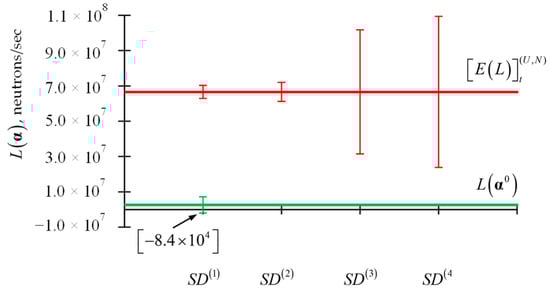
Figure 2.
Comparison of (in green), (in red), due to 10% standard deviations of the uncorrelated microscopic total cross sections.
In summary, the impact of the sensitivities of various orders on the standard deviation of the leakage response is as follows: (i) for small (1%) relative standard deviations for the microscopic total cross sections, the uncertainty of the leakage response arising solely from the first-order sensitivities are significantly larger than the uncertainties arising solely from the second-, third-, and fourth-order sensitivities, respectively, but following an oscillating pattern: ; (ii) when considering moderate (5%) and larger (10%) relative standard deviations for the microscopic total cross sections, the standard deviation of the leakage response increases substantially as successively higher-order sensitivities are considered, leading to the following sequence of inequalities, , which indicates the need to verify the convergence/divergence of the Taylor series which underlies the expression of the response’s standard deviation.
3.1.3. Effects of the Fourth-Order Sensitivities on the Third-Order Response Moment and Skewness
The results obtained for the third-order response moment and skewness when considering relative standard deviations of 1%, 5%, and 10%, respectively, for the microscopic total cross sections (considered to be normally distributed and uncorrelated) are summarized in Table 5.
Table 5.
Comparison of the third-order response moment and skewness for various relative standard deviations (RSD) of the normally distributed and uncorrelated microscopic total cross sections.
Considering 1% relative standard deviations for the uncorrelated microscopic total cross sections, the results presented in Table 5 indicate that , , and . Thus, for small (1%) relative standard deviations, the contributions to the third-order response moment stemming from the second-order sensitivities are the largest (e.g., around 53% in this case), followed by the contributions stemming from the third-order sensitivities, while the contributions stemming from the fourth-order sensitivities are the smallest.
Considering 5% relative standard deviations for the uncorrelated microscopic total cross sections, the results in Table 5 show that , , and . In this case, the contributions from the third-order sensitivities are the largest (e.g., around 60%), followed by the contributions from the fourth-order sensitivities, which contribute about 30%; the smallest contributions stem from the second-order sensitivities.
Considering 10% relative standard deviations for the uncorrelated microscopic total cross sections, the results in Table 5 indicate that , , and . These results display the same trends as the results for the “RSD = 5%” case, but the magnitudes of the respective contributions are significantly larger by comparison to the corresponding results for the “RSD = 5%” case.
For the response skewness, , the results shown in in the last row of Table 5 indicate that all the second-, third-, and fourth-order sensitivities produce a positive response skewness, which causes the leakage response distribution to be skewed towards the positive direction from its expected value . The results shown in the last row of Table 5 also indicate that as the relative standard deviation of the uncorrelated microscopic total cross sections increases from 1% to 10%, the value of the skewness decreases, thus causing the leakage response distribution to become increasingly more symmetrical about the mean value . Neglecting the fourth-order sensitivities would cause a significant error in the skewness. For example, for the case “RSD = 5%”, if the fourth-order sensitivities were neglected, the contributions from the first-, second-, and third-order sensitivities to the skewness would have the value , which would be 135% smaller than the more accurate result obtained by including the contributions of the fourth-order sensitivities. The fourth-order sensitivities produce a positive response skewness, causing the leakage response distribution to be skewed towards the positive direction from its expected value. The impact of the fourth-order sensitivities on the skewness of the leakage response also changes with the value of the standard deviation of the microscopic total cross sections: larger standard deviations (for the parameters) tend to decrease the value of the skewness, causing the leakage response distribution to become more symmetrical about the mean value .
A “first-order sensitivity and uncertainty quantification” will always produce an erroneous third moment (and, hence, skewness) of the predicted response distribution, unless the unknown response distribution happens to be symmetrical. At least second-order sensitivities must be used in order to estimate the third-order moment (and, hence, the skewness) of the response distribution. With pronounced skewness, standard statistical inference procedures such as constructing a confidence interval for the mean (expectation) of a computed/predicted model response will be not only incorrect, in the sense that the true coverage level will differ from the nominal (e.g., 95%) level, but the error probabilities will be unequal on each side of the predicted mean. Thus, the truncation of Taylor expansion of the response (as a function of parameters) depends both on the magnitudes of the response sensitivities to parameters and the parameter uncertainties involved: if the uncertainties are small, then a fourth-order expansion suffices, in most cases, for obtaining relatively accurate results. In any case, the truncation error of a convergent Taylor series can be quantified a priori. If the parameter uncertainties are large, the Taylor series may diverge, so one would need to reduce such uncertainties, e.g., by performing additional measurements of the respective parameters. Of course, if the parameter uncertainties are large, all statistical methods are doomed to produce unreliable results for large-scale, realistic problems involving many uncertain parameters.
Obtaining the exact and complete set of first-order sensitivities of responses to model parameters is therefore of paramount importance for any analysis of a computational model. The second-order sensitivities contribute the leading correction terms to the response’s expected value, causing it to differ from the response’s computed value. The second-order sensitivities also contribute to the response variances and covariances. If the parameters follow a normal (Gaussian) multivariate distribution, the second-order sensitivities contribute the leading terms to the response’s third-order moment. In particular, the skewness of a single response, , is customarily denoted as , and is defined as follows: where denotes the third central moment of the response distribution. Thus, neglecting the second-order response sensitivities to normally distributed parameters would nullify the third-order response correlations and hence would nullify the skewness of a response. Hence, a “first-order sensitivity and uncertainty quantification” will always produce a zero-valued skewness of the predicted response distribution, which would be erroneous unless the unknown response distribution happens to be symmetrical. At least second-order sensitivities must be used in order to estimate the third-order moment and, hence, the skewness of the response distribution. The skewness provides a quantitative measure of the asymmetries in the respective distribution, indicating the direction and relative magnitude of a distribution’s deviation from the normal distribution. With pronounced skewness, standard statistical inference procedures such as constructing a confidence interval for the mean (expectation) of a computed/predicted model response will be incorrect, in the sense that the true coverage level will differ from the nominal (e.g., 95%) level. Furthermore, the error probabilities will be unequal on each side of the predicted mean.
3.2. Overview of the nth-Order Comprehensive Adjoint Sensitivity Analysis Methodology for Response-Coupled Forward and Adjoint Linear Systems (nth-CASAM-L)
The nth-Order Comprehensive Adjoint Sensitivity Analysis Methodology for Response-Coupled Forward and Adjoint Linear Systems (nth-CASAM-L), which was originally presented by Cacuci [36], is briefly summarized in this subsection. As was mentioned in Section 3.1, the mathematical/computational model of a physical system comprises model parameters which are imprecisely known. In addition to the TP model parameters described in Section 3.1, the mathematical model of a physical system is considered to comprise independent variables which will be denoted as , and are considered to be the components of a -dimensional column vector denoted as , where the sub/superscript “” denotes the “Total (number of) Independent variables” and where the components , can be considered, without loss of generality, to be real quantities. The vector of independent variables is considered to be defined on a phase-space domain, denoted as , , the boundaries of which may depend on (some of) the model parameters . The lower boundary point of an independent variable is denoted as (e.g., the inner radius of a sphere or cylinder, the lower range of an energy variable, the initial time value, etc.), while the corresponding upper boundary point is denoted as (e.g., the outer radius of a sphere or cylinder, the upper range of an energy variable, the final time value, etc.). The boundary of is denoted as ; it comprises the set of all of the endpoints , .
A linear physical system is generally modeled by a system of coupled linear operator equations which can be generally represented in block-matrix form, as follows:
where is a -dimensional column vector of dependent variables and where the sub/superscript “” denotes the “Total (number of) Dependent variables.” The functions , denote the system’s “dependent variables” (also called “state functions”). The components , , of the -dimensional matrix are operators that act linearly on the dependent variables and also depend on the uncertain model parameters . The components of the -dimensional column vector represent inhomogeneous source terms which are considered to depend (nonlinearly) on the model parameters. Since the sources on the right side of Equation (27) may comprise distributions, all equalities that involve differential equations are considered to hold in the weak (i.e., “distributional”) sense.
Since the complete mathematical model is considered to be linear in , the boundary and/or initial conditions needed to define the domain of ; when contains differential operators, it must also be linear in and can be represented as follows:
In (28), the components , of the -dimensional matrix operator act linearly on and nonlinearly on . The total number of boundary and initial conditions is denoted as . The operator is a -dimensional vector comprising inhomogeneous boundary source terms that act nonlinearly on . The subscript “” in Equation (28) indicates boundary conditions associated with the forward state function .
Physical problems modeled by linear systems and/or operators are naturally defined in Hilbert spaces. The dependent variables , for the physical system represented by Equations (27) and (28) are considered to be square-integrable functions of the independent variables, belonging to a Hilbert space which is denoted as (where the subscript “zero” denotes “zeroth-level“ or “original”). The Hilbert space is considered to be endowed with the following inner product, denoted as , between two elements and :
The product notation in Equation (29) denotes the respective multiple integrals. The linear operator admits an adjoint operator, which is denoted as and which is defined through the following relation for a vector :
In (30), the formal adjoint operator is the matrix comprising elements obtained by transposing the formal adjoints of the forward operators , i.e.,
Hence, the system adjoint to the linear system represented by (27) and (28) can generally be represented as follows:
When comprises differential operators, the operations (e.g., integration by parts) that implement the transition from the left side to the right side of Equation (30) give rise to boundary terms which are collectively called the “bilinear concomitant.” The domain of is determined by selecting adjoint boundary and/or initial conditions so as to ensure that the bilinear concomitant vanishes when the selected adjoint boundary conditions are implemented together with the forward boundary conditions given in Equation (28). The adjoint boundary conditions thus selected are represented in operator form by Equation (33), where the subscript “” indicates adjoint boundary and/or initial conditions associated with the adjoint state function . In most practical situations, the Hilbert space is self-dual. Solving Equations (27) and (28) at the nominal parameter values yields the nominal value of the forward state function, while solving Equations (32) and (33) at yields the nominal value of the adjoint state function.
The relationship shown in Equation (30), which is the basis for defining the adjoint operator, also provides the following fundamental “reciprocity-like” relation between the sources of the forward and the adjoint equations, cf. Equations (27) and (32), respectively:
The functional on the right side of Equation (34) represents a “detector response”, i.e., a reaction rate between the particles and the medium represented by , which is equivalent to the “number of counts” of particles incident on a detector of particles that “measures” the particle flux . In view of the relation provided in Equation (34), the source term in the adjoint Equation (32) is usually associated with the “result of interest” to be measured and/or computed, which is customarily called the system’s “response.” In particular, if , then , which means that, in such a case, the right side of (34) provides the value of the dependent variable (particle flux, temperature, velocity, etc.) at the point in the phase space where the respective measurement is performed.
Since the linear operators that underly linear systems admit adjoint operators, important model responses of linear systems can be functions of both the forward and the adjoint state functions. Examples of such responses are the Schwinger [37] and Roussopoulos [38] functionals, as well as the Raleigh quotient [39] for computing eigenvalues of linear systems. Such responses cannot be encountered in nonlinear problems since nonlinear operators do not admit adjoint operators. In this sense, linear systems differ fundamentally from nonlinear systems and cannot always be considered to be particular cases of nonlinear systems but need to be treated comprehensively in their own right. Thus, the fundamental form of a response computed using a linear model is an operator which acts nonlinearly on the model’s forward and adjoint state functions, as well as on the imprecisely known model parameters, directly and indirectly through the state functions, having the following generic form:
where denotes a suitably Gateaux (G)-differential function of the indicated arguments. In general, is nonlinear in , , and , and the components of are considered to also include parameters that may specifically appear only in the definition of the response under consideration (but which might not appear in the definition of the model). Thus, the (physical) “system” is defined and understood to comprise both the system’s computational model and the system’s response. Due to the response’s implicit dependence on the model parameters through the forward and/or adjoint state functions, the response of a linear system is a nonlinear function of the model’s parameters, except perhaps in particularly trivial situations. The nominal value of the response, , is determined by using the nominal parameter values , the nominal value of the forward state function, and the nominal value of the adjoint state function.
Since the model parameters are imprecisely known quantities, their actual values (which are not known in practice) will differ from their nominal values (which are known in practice) by quantities denoted as The variations will cause corresponding variations ,, in the forward and adjoint state functions, respectively. In turn, all of these variations will cause a response variation around the nominal value . The first-order sensitivities of the response with respect to the model parameters are contained within the first-order Gateaux (G)-variation, denoted as , of the response for arbitrary variations in the model parameters and state functions, in a neighborhood around . By definition, the first-order Gateaux (G)-variation is obtained as follows:
where the “direct-effect” term depends only on the parameter variation and is defined as follows:
and where the “indirect effect” term depends only on the variations and in the state functions, and is defined as follows:
The notation has been used in Equations (37) and (38) to indicate that the quantity within the brackets is to be evaluated at the nominal values of the parameters and state functions. While the “direct effect” term defined in Equation (37), which depends only on the parameter variations , can be computed immediately, the “indirect effect” term defined in Equation (38) can be computed only after having determined the values of the variations and . The variations and are the solutions of the system of equations obtained by taking the G-differentials of Equations (27), (28), (32), and (33), which can be written in the following matrix-vector form:
where
The matrices and , which appear on the right side of Equation (39), are defined as follows:
The system of equations comprising Equations (39) and (40) is called the “1st-Level Variational Sensitivity System” (1st-LVSS) and its solution, , is called the “1st-Level variational sensitivity function”, as indicated by the superscript “(1)”. Since the source term, , is a function of , it follows that the 1st-LVSS would need to be solved times in order to obtain the vector which would correspond to each parameter variation , . The need for computing the functions and can be avoided by applying the First-Order Comprehensive Adjoint Sensitivity Analysis Methodology (1st-CASAM-L), which enables the elimination of and from the expression of the indirect effect term defined in Equation (38). This elimination is achieved by implementing the following sequence of steps:
- Introduce a Hilbert space, denoted as , comprising square-integrable function vector-valued elements of the form , , . The inner product between two elements, , , is denoted as and is defined as follows:
- In the Hilbert , form the inner product of Equation (39) with a vector-valued function to obtain:
- Using the definition of the adjoint operator in the Hilbert space , recast the left side of Equation (46) as follows:where denotes the bilinear concomitant defined on the phase-space boundary , and where is the operator formally adjoint to , defined as follows:
- Require the first term on right side of Equation (47) to represent the indirect effect term defined in Equation (38), to obtain the following relation:where
- Implement the boundary conditions given in Equation (40) into Equation (47) and eliminate the remaining unknown boundary values of the functions and from the expression of the bilinear concomitant by selecting appropriate boundary conditions for the function , to ensure that Equation (49) is well-posed while being independent of unknown values of , , and . The boundary conditions thus chosen for the function can be represented in operator form as follows:
- The selection of the boundary conditions for the adjoint function represented by Equation (51) eliminates the appearance of the unknown values of in the bilinear concomitant and reduces it to a residual quantity which will be denoted as and which contains boundary terms involving only known values of , , , , and . This residual quantity does not automatically vanish.
- The system of equations comprising Equation (49) together with the boundary conditions represented in Equation (51) constitute the First-Level Adjoint Sensitivity System (1st-LASS). The solution of the 1st-LASS is called the First-level adjoint sensitivity function. The 1st-LASS is called “first-level” (as opposed to “first-order”) because it does not contain any differential or functional derivatives, but its solution, , is used below to compute the first-order sensitivities of the response with respect to the model parameters.
- It follows from (46) and (47) that the following relation holds:
- Recalling from (49) that the first term on the right side of (52) is the indirect effect term , it follows from (52) that the indirect effect term can be expressed in terms of the first-level adjoint sensitivity function as follows:
As indicated by the identity relation in Equation (53), the variations and have been eliminated from the original expression of the indirect effect term, which now instead depends on the first-level adjoint sensitivity function . Very importantly, the 1st-LASS is independent of parameter variations . Hence, the 1st-LASS needs to be solved only once (as opposed to the 1st-LVSS or the 1st-OFSS, which would need to be solved anew for each parameter variation) to determine the first-level adjoint sensitivity function . Subsequently, the indirect effect term is computed efficiently and exactly by simply performing the integrations over the adjoint function , as indicated by Equation (53).
Adding the expression of the direct effect term defined in Equation (37) to the expression of the indirect effect term obtained in Equation (53) yields the following expression for the total first-order G-differential of the response computed at the nominal values for the models’ parameter and state functions:
The expression obtained in Equation (54) no longer depends on the variations and but instead depends on the first-level adjoint sensitivity function . In particular, the expression in Equation (54) reveals that the sensitivities of the response to parameters that characterize the system’s boundary and/or internal interfaces can arise both from the direct effect and indirect effect terms. It also follows from Equation (54) that the quantity has become a total differential in the parameter variation so it can be expressed in the following form:
where the quantities represent the first-order sensitivities (i.e., partial functional derivatives) of the response with respect to the model parameter , evaluated at the nominal values of the state functions and model parameters. Furthermore, each of the first-order sensitivities can be represented in integral form as follows:
In particular, if the residual bilinear concomitant does not vanish, the functions would contain suitably defined Dirac delta functionals for expressing the respective non-zero boundary terms as volume integrals over the phase space of the independent variables. Dirac delta functionals would also be needed to represent, within , the terms containing the derivatives of the boundary endpoints with respect to the model and/or response parameters.
Cacuci [36] has obtained the general expression of the arbitrarily high-order (nth-order, where n is an arbitrary integer) sensitivities of the response to model parameters by treating each sensitivity as a response, applying the principles outlined in items (1)−(9) to successively higher-order sensitivities and, ultimately, using mathematical induction to demonstrate that general expression thus obtained for the nth-order sensitivity is correct. Each of the (n − 1)th-order sensitivities of the response with respect to the parameters , where , are used in the role of a “model response”, for which the first-order G-differential is obtained by applying the principles outlined in items (1)−(9), thereby ultimately obtaining the general expression of the nth-order sensitivities of the response . The details of the nth-CASAM-L methodology are provided by Cacuci [36]. The end results produced by the nth-CASAM-L methodology enable the exact and efficient computation—overcoming the curse of dimensionality in sensitivity analysis—of the nth-order partial sensitivities of the response with respect to the model parameters, using the expression provided below:
The various quantities which appear in Equation (57) are defined as follows:
- (1)
- The quantity denotes the nth-order partial sensitivity of the response with respect to the model parameters, evaluated at the nominal values of the parameters and state functions. When the symmetries among the various partial derivatives/sensitivities are considered, the respective indices have ranges as follows: ; ; …; . In integral form, the nth-order partial sensitivity of the response can be written as follows:
- (2)
- The nth-level state , which appears in the arguments of , is defined as follows:
- (3)
- The inner product which appears in Equation (57) is defined in a Hilbert space denoted as , comprising -dimensional block vectors having the following structure: ,, . The inner product between two elements, and , of the Hilbert space , is denoted as and is defined as follows:
- (4)
- The adjoint operator which appears on the left side of Equation (62) is constructed by using the inner product defined in Equation (60), via the following relation:
- (5)
- The nth-level adjoint sensitivity function , which appears in the arguments of , is the solution of the following nth-level adjoint sensitivity system nth-LASS, for ; ; …:where the vector , comprises components defined for each ; ; …; , as follows:
- (6)
- The quantity denotes the residual bilinear concomitant defined on the phase-space boundary , evaluated at the nominal values of the model parameter and respective state functions.
4. High-Order Sensitivity and Uncertainty Analysis of Nonlinear Models/Systems: Illustrative Example and General Theory
It is currently well known that a boiling water reactor (BWR) can undergo time-dependent power–amplitude oscillations, particularly when operated under high-power and low-flow conditions, due to the nonlinear coupling, through the void reactivity, between the neutronics and thermal-hydraulic processes. Such power oscillations can occur globally, when the reactor’s power oscillates in phase across the entire reactor core, or regionally, when part (e.g., half, for the so-called “first mode”) of the reactor core oscillates out of phase with respect to the other part (half), while the average power remains essentially constant across the reactor. In a pioneering sequence of works, March-Leuba, Cacuci, and Perez [45,46,47] proposed a phenomenological reduced-order model for analyzing qualitatively the dynamic behavior of BWRs, predicting global limit cycle oscillations in BWRs four years before they actually occurred [62] in an operating power reactor in the USA, on 9 March 1988, in the LaSalle County-2 BWR in Seneca, Illinois. The reduced-order model developed by March-Leuba, Cacuci, and Perez [45] comprises point neutron kinetics equations coupled nonlinearly to thermal-hydraulics equations that describe the time evolution of the fuel temperature and coolant density in the recirculation loop, which is treated as a single path of fluid of variable cross-sectional area but with constant mass flow, with the coolant entering the core at saturation temperature. This model showed that the major state variables, including power, reactivity, void fraction, and temperature, undergo limit cycle oscillations under high-power/low-flow operating conditions, and the amplitudes of these oscillations are very sensitive to the reactor’s operating conditions. This model also indicated that these limit cycle oscillations can become unstable—when increasing the heat transfer from the reactor to the coolant—and can undergo period-doubling bifurcations causing oscillatory (from periodic to aperiodic) time evolutions of the state variables (power, delayed neutron precursors, reactivity, coolant void fraction, and fuel temperature). The reduced-order model introduced by March-Leuba, Cacuci, and Perez [45] has generated great interest in the scientific community, inspiring investigations of the stability limits for in-phase and out-of-phase oscillation modes and the nature of the underlying bifurcations in the various state functions, as exemplified by [48,49,50,51,52,53,54,55].
Section 4.1 reviews the pioneering sensitivity and uncertainty analysis results presented in [43,44] for the reduced-order model of BWR dynamics developed by March-Leuba, Cacuci, and Perez [45]. This nonlinear model [45] illustrates generically the most extreme forms of nonlinear phenomena (from limit cycles to chaos) that can be displayed by nonlinear physical systems, so it is considered to be a representative paradigm for illustrating the application of the nth-CASAM-N methodology [42] for computing efficiently and exactly the sensitivities of responses to parameters for nonlinear systems. For completeness, the general mathematical formalism underlying the nth-CASAM-N [42] is reviewed in Section 4.2.
4.1. Illustrative Sensitivity and Uncertainty Analysis of a Reduced-Order Model of BWR-Dynamics
The reduced-order model developed by March-Leuba, Cacuci, and Perez [45] describes the fundamental processes underlying the dynamic behavior of a BWR when the reactor is perturbed from its originally critical steady-state condition, by insertion of reactivity. This reduced-order (lumped-parameter) model comprises differential equations that describe the following phenomena:
- (a)
- A point reactor representation of neutron kinetics, including the neutron precursors:
- (b)
- A “one-node” lumped-parameter representation of the heat transfer process in the fuel:
- (c)
- A “two-nodes” lumped-parameter representation of the channel thermal hydraulics, accounting for the reactivity feedback:
The initial conditions at for Equations (74)−(77) are as follows:
The state variables in Equations (74)−(78) are defined as follows:
- (i)
- denotes the normalized excess neutron population, where denotes the actual time-dependent neutron population and denotes the neutron population of the initially critical reactor.
- (ii)
- denotes the normalized excess population of delayed neutron precursors, where denotes the actual time-dependent population of delayed neutron precursors and denotes the population of delayed neutron precursors of the initially critical reactor.
- (iii)
- denotes the excess fuel temperature, defined as the departure from the temperature of the initially critical reactor.
- (iv)
- denotes the Heaviside functional: and .
- (v)
- denotes the relative excess coolant density, defined as the departure from the coolant density of the initially critical reactor.
- (vi)
- denotes the excess reactivity, defined as the departure from the reactivity of the initially critical reactor.
The nominal values of the model parameters which appear in Equations (74)−(78) are reported in Table 6. Since the qualifier “excess” signifies that the above quantities are defined as departures from the critical reactor configuration, the nominal values of the initial conditions shown in Equations (79)−(82) are all zero at .
Table 6.
Nominal values of imprecisely known BWR model parameters.
The reduced-order model defined by Equations (74)−(82) has two equilibrium points in the phase space, one stable (denoted as “point A”) and the other one unstable (denoted as “point B”), at the following phase space locations:
- Stable equilibrium (A), which corresponds to the critical reactor configuration, which is defined as follows:
- b.
- Unstable equilibrium (B):
As discussed by March-Leuba, Cacuci, and Perez [45], when the feedback gain in Equation (77) is increased, thereby increasing the heat transfer from the reactor to the coolant, the equilibrium point A becomes unstable after the stability threshold is crossed. The phase-space trajectories of the lumped-parameter model oscillate between the two unstable equilibrium points until a stable limit cycle sets in. Increasing the value of the feedback gain beyond the stability of the first limit cycle will cause this cycle to bifurcate, through a period-doubling bifurcation, into a period-two cycle. Continuing to increase the feedback gain leads to a cascade of period-doubling bifurcations which lead to aperiodic behavior, as illustrated in Figure 3 by the bifurcation map for the excess temperature , which is obtained by plotting the extrema of as a function of the feedback gain . The values of the bifurcation variables are provided in Table 7. The bifurcation map presented in Figure 3 for values of k ranging from to (i.e., ) highlight the following Regions in the phase space:
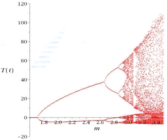
Figure 3.
Bifurcation map of .
Table 7.
Bifurcation points for the reduced-order BWR model by March-Leuba, Cacuci, and Perez (1984).
- Region 1: Stable Region, before the first-order bifurcation, , in which the state functions oscillate with decreasing amplitudes converging toward steady-state values.
- Region 2: Unstable Region between the first-order bifurcation and the second-order bifurcations, , in which the state functions oscillate indefinitely between two unstable attractors.
- Region 3: Unstable Region between the second-order bifurcations and the third-order bifurcations, , in which the state functions oscillate indefinitely between four unstable attractors.
- Region 4: Unstable Region between the third-order bifurcations and the fourth-order bifurcations, , in which the state functions oscillate indefinitely between eight unstable attractors.
- Region 5: Chaotic Region stemming from the cascade of period-doubling pitchfork bifurcations produced when the feedback gain is increased past a critical value (called accumulation point), , where , in which the state functions oscillate indefinitely between infinitely many unstable attractors.
The state functions are attracted in the stable Region 1 to the stable equilibrium attractor A, having the following coordinates in the phase space:
The largest first-order sensitivity displayed by is with respect to the initial condition for the excess coolant density , as depicted in Figure 4, which also presents, for comparison, the sensitivities of to the other initial conditions. As depicted in Figure 4, the sensitivities oscillate with very large amplitudes immediately after the onset of the transient, which is initiated by perturbing the initially critical reactor in the steady state, and these amplitudes decay exponentially in time. The features depicted in Figure 4 are transmitted to the first-order total absolute standard deviation, denoted as , induced in by the sensitivities and parameter standard deviations, as shown in Figure 5.
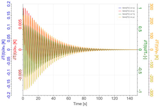
Figure 4.
Time evolutions of the sensitivities of with respect to the initial conditions , , , in Region 1.
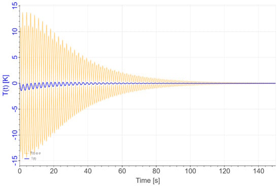
Figure 5.
Time evolution of (blue graph) with uncertainty bands (yellow graphs), considering uniform 5% relative standard deviations for all parameters and 5% absolute standard deviations for the initial conditions in Region 1.
The first-order total absolute standard deviation, denoted as , for is obtained by using the well-known formula , where denotes the sensitivity of to the parameter , and where denotes the standard deviation for the respective parameter. The time evolution of the nominal value of the state function is depicted in blue in Figure 5 along with the time evolution of the functions labeled “” and depicted in yellow, where denotes the total absolute standard deviation for . Immediately after the onset of the transient effected by perturbing the initially critical reactor in the steady state, the standard deviation for is very large, reaching values that more than 10 times larger than the state function itself. In time, the standard deviation decays exponentially, reaching values comparable to the state function after about 140 s from the start of the transient. Very importantly, Figure 5 indicates that predictions of the excess temperature of during the first 120 s after the BWR model is perturbed from its initial critical steady state would be unreliable. Furthermore, it is possible that that the model could be “pushed” into one of the oscillatory Regions by the large amplitudes reached by the standard deviation of immediately after the onset of the perturbation.
The largest first-order sensitivity displayed by in the oscillatory Region 2 is also with respect to the initial condition ; the time evolution of this sensitivity is depicted in Figure 6, together with the sensitivities of to the other initial conditions. As depicted in Figure 6, the amplitudes of these sensitivities are about two orders of magnitude larger than the corresponding first-order sensitivities. In contradistinction with the decaying amplitudes of the oscillations in Region 1, the oscillation amplitudes of the sensitivities in Region 2 stabilize to large values asymptotically in time. The features depicted in Figure 6 are transmitted to the first-order total absolute standard deviation induced in , as shown in Figure 7, which depicts (in blue) the time evolution of the nominal value of the state function along with the time evolution (in yellow) of the functions . As indicated in Figure 7, the standard deviation increases rapidly after the onset of the transient (by perturbing the initially critical reactor in the steady state), oscillating with rapidly increasing amplitudes, reaching in 40 s after the start of the transient values that are 400K larger than the amplitude of the excess temperature, , which oscillates around the initial value . It is evident from Figure 7 that the standard deviation of renders the prediction of the evolution of this state function highly unreliable after less than 10 s from the initiation of the transient.
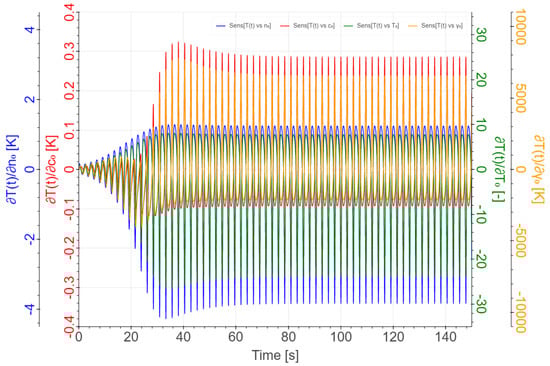
Figure 6.
Time evolutions of the sensitivities of with respect to the initial conditions , , , in Region 2.
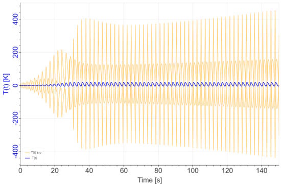
Figure 7.
Time-evolution of (blue graph) with uncertainty bands (yellow graphs), considering uniform 5% relative standard deviations for all parameters and 5% absolute standard deviations for the initial conditions in Region 2.
The evolution of the standard deviation of in the oscillatory Region 3 is depicted in Figure 8, which indicates that a standard deviation as small as 5% in the model’s parameters and initial conditions will be magnified in the oscillatory regions so much as to preclude any accurate prediction of the actual values of the excess temperature . This conclusion is also evidenced by the results presented in Table 8, which presents the largest positive and negative values attained by the oscillation amplitude of in the aperiodic Region 5, for 6 windows of 25 s each, covering the transient period from 0 to 150 s.
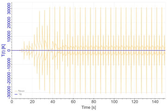
Figure 8.
Time-evolution of (blue graph) with uncertainty bands (yellow graphs), considering uniform 5% relative standard deviations for all parameters and 5% absolute standard deviations for the initial conditions in Region 3 for .
Table 8.
Maxima and minima of the uncertainty of considering a 5% std. dev. for all parameters and initial conditions in Region 5 for various time windows.
4.2. Overview of the nth-Order Comprehensive Sensitivity Analysis Methodology for Nonlinear Systems (nth-CASAM-N)
Using the same notation for the model’s independent variables and parameters as for the linear system considered in Section 3, the mathematical modeling of a nonlinear physical system can be represented in operator form as follows:
The quantities which appear in Equation (86) are defined as follows:
- is a -dimensional column vector of dependent variables; the abbreviation “” denotes “total number of dependent variables.” The functions denote the system’s “dependent variables” (also called “state functions”); , where is a normed linear space over the scalar field of real numbers.
- denotes a -dimensional column vector. The components are operators (including differential, difference, integral, distributions, and/or finite or infinite matrices) acting (usually) nonlinearly on the dependent variables , the independent variables , and the model parameters . The mapping is defined on the combined domains of the model’s parameters and state functions, i.e., , where , , , .
- is a -dimensional column vector which represents inhomogeneous source terms, which usually depend nonlinearly on the uncertain parameters . The vector is defined on a normed linear space denoted as , i.e., .
Boundary and/or initial conditions must also be provided if differential operators appear in Equation (86). In operator form, these boundaries and/or initial conditions are represented as follows:
Solving Equations (86) and (87) at the nominal parameter values provides the “nominal solution” , i.e., the vectors and , satisfies the following equations:
The model response is a functional considered to be representable in the following generic integral form:
where is a suitably differentiable nonlinear function of and of . It is important to note that the components of include not only parameters that appear in the equations defining the computational model per se, i.e., in Equations (86) and (87), but also include parameters that specifically occur only in the definition of the response under consideration. It is also important to note that the system’s definition domain, , in phase space is considered to be imprecisely known, subject to uncertainties in the components of the vector of model parameters . Therefore, the system domain’s boundary, , as well as the model response , will be affected by the boundary uncertainties that affect the endpoints . Such boundary uncertainties stem most often from manufacturing uncertainties.
Variation in the model and boundary parameters will cause corresponding variations around the nominal solution in the forward state functions. The variations and will, in turn, induce variations in the system’s response. The first-order G-differential is obtained, by definition, as follows:
In Equation (91), the direct effect term comprises only dependencies on and is defined as follows:
where
On the other hand, the quantity in Equation (91) comprises only variations in the state functions and is therefore called the indirect effect term, having the following expression:
The indirect effect term induces variations in the response through the variations in the state functions, which are, in turn, caused by the parameter variations through the equations underlying the model. Evidently, the indirect effect term can be quantified only after having determined the variation in terms of the variation . The indirect effect term induces variations in the response through the variations in the state functions, which are, in turn, caused by the parameter variations through the equations underlying the model. Evidently, the indirect effect term can be quantified only after having determined the variation in terms of the variation .
The first-order relationship between the vectors and is determined by solving the equations obtained by applying the definition of the G-differential to Equations (86) and (87), which yields the following equations:
Carrying out the differentiations with respect to in Equations (95) and (96) and setting in the resulting expressions yields the following equations:
In Equations (97) and (98), the superscript “(1)” indicates “1st-Level” and the various quantities which appear in these equations are defined as follows:
The system comprising Equations (97) and (98) is called the “1st-Level Variational Sensitivity System” (1st-LVSS). In order to determine the solutions of the 1st-LVSS that would correspond to every parameter variation , , the 1st-LVSS would need to be solved times, with distinct right sides for each , thus requiring large-scale computations.
The need for computing the vector is eliminated by applying the 1st-CASAM-N to express the indirect effect term defined in Equation (94) in terms of the solutions of the “1st-Level Adjoint Sensitivity System” (1st-LASS), the construction of which requires the introduction of adjoint operators. The 1st-CASAM-N represents a generalization of the pioneering works by Cacuci (1981a, b) which had conceived the “Adjoint Sensitivity Analysis Methodology for Nonlinear Systems” but in which the domain boundary was considered to have been perfectly well-known, free of uncertainties. The qualifier “comprehensive” is meant to indicate that that the 1st-CASAM-N considers that the internal and external boundaries of the phase-space domain depend on the uncertain model parameters and are thereby imprecisely known, subject to uncertainties. The construction of the “1st-Level Adjoint Sensitivity System” (1st-LASS) is accomplished by introducing a real Hilbert space denoted as , endowed with an inner product of two vectors and denoted as and defined as follows:
where , and where the “dagger” (), which indicates “transposition”, has been omitted (to simplify the notation) in the representation of this scalar product. Using the definition of the adjoint operator in and applying the 1st-CASAM-N yields the following expression for the first G-differential of the response :
where for each , the quantity denotes the first-order sensitivities of the response with respect to the model parameters and has the following expression:
The quantity , which appears in the inner product on the right side of Equation (105), is defined as follows:
The first-level adjoint sensitivity function , which appears in the inner product on the right side of Equation (105), is the solution of the following 1st-LASS:
In Equations (107) and (108), the superscript “(1)” indicates “1st-Level”, (evidently), and the various quantities which appear in these equations are defined as follows:
The domain of the first-level adjoint operator is determined by selecting adjoint boundary and/or initial conditions, represented in operator form in Equation (108), such as to eliminate boundary terms containing unknown values of the function which arise in the bilinear concomitant in the course of constructing through the following relation:
where denotes the associated bilinear concomitant evaluated on the space/time domain’s boundary . The selection of the adjoint boundary conditions represented by Equation (108) reduces the bilinear concomitant to a quantity denoted as , which will contain boundary terms involving only known values of , , , and .
As indicated by Equation (105), each of the first-order sensitivities of the response with respect to the model parameters (including boundary and initial conditions) can be computed inexpensively after having obtained the function , using just quadrature formulas to evaluate the various inner products involving . The function is obtained by solving numerically the 1st-LASS, cf. Equations (107) and (108), which is the only large-scale computation needed for obtaining all of the first-order sensitivities, since the 1st-LASS is independent of parameter variation , , and therefore needs to be solved only once, regardless of the number of model parameters under consideration. Furthermore, since the 1st-LASS is linear in , solving it requires less computational effort than solving the original model, which is nonlinear in . The first-order sensitivity is used in the role of a “model response” for determining the second- and higher-order sensitivities of the response with respect to the model’s parameters.
The generic expression of the nth-order sensitivity of the response with respect to the parameters is obtained, for each , by applying the nth-Order Comprehensive Sensitivity Analysis Methodology for Nonlinear Systems (nth-CASAM-N) conceived by Cacuci [40]. Using mathematical induction, Cacuci [40] obtained the nth-order sensitivity from the expression of the total first-order G-differential of each of the (n − 1)th-order sensitivities, each of which was shown by Cacuci [40] to have the following expression for :
where
The various quantities appearing in the expression presented in Equation (113) are defined as follows:
- (i)
- The nth-level adjoint sensitivity function , which appears in the inner product on the right side of Equation (113), is the solution of the following nth-Level Adjoint Sensitivity System (nth-LASS):subject to boundary conditions represented in operator form as follows:The quantities which appear in the definition of the nth-LASS, cf. (115) and (116), are defined as follows:The variational matrix comprises block matrices, each comprising components/elements. Thus, the matrix comprises a total of components/elements. The quantity denotes a block matrix having components, each component being a -dimensional matrix having identically zero components. The other submatrices appearing in the definition of are as follows:
- (ii)
- The quantity , which appears in the inner product on the right side of Equation (113), is defined as follows:
- (iii)
- The inner product which appears on the right side of Equation (113) is defined in a Hilbert space , the elements of which are block vectors of the form , comprising -dimensional vectors of the form , . The Hilbert space is endowed with an inner product of two vectors and , denoted as and defined as follows:
- (iv)
- The nth-Level Adjoint Sensitivity System (nth-LASS) for the nth-level adjoint function is obtained by using the inner product defined in (128), as follows:where the quantity denotes the corresponding bilinear concomitant on the domain’s boundary, evaluated at the nominal values for the parameters and respective state functions.
- (v)
- The quantity , which appears on the right side of Equation (113), denotes residual boundary terms which may have not vanished automatically after having used the variational forward and adjoint boundary conditions to eliminate from Equation (129) all unknown values of the nth-level variational function .
5. Discussion: Unified View of the nth-CASAM-L and nth-CASAM-N Methodologies
As indicated by the summary presentations in Section 3 and Section 4, the nth-CASAM-L and nth-CASAM-N methodologies are based on the same fundamental principles, as follows:
- The total sensitivity of a model response to the model parameters is defined as the Gateaux (G)-differential of the response with respect to variations in the model parameters and state functions, thereby giving rise to two terms: (i) the so-called direct effect term, which depends directly and solely on the variations in the model parameters, and (ii) the so-called indirect effect term, which depends solely on the variations in the model’s state functions.
- The straightforward evaluation of the indirect effect term would require performing as many large-scale computations (equivalent to solving the original equations) as there are model parameters, which is computationally impractical/unfeasible for realistic models involving many parameters.
- The need for performing impractically many large-scale computations is overcome by replacing the state function variations in the expression of the indirect effect term with the first-level adjoint sensitivity function, the computation of which requires a single large-scale computation for solving the 1st-LASS, which is independent of parameter variations.
- Each subsequent sensitivity is treated as a model response, i.e., the first-order sensitivities are considered to be model responses for the computation of the second-order sensitivities using second-level adjoint sensitivity functions, and so on. The dimensions of the nth-LASS increase linearly with the order n of the computed sensitivity.
- The sensitivities of order higher than first are computed in the ranking order of the first-order sensitivities, starting with the second-order sensitivities stemming from the largest first-order sensitivity, which are computed with the highest priority.
- Since the linear operators that underly linear systems admit adjoint operators, important model responses of linear systems can be functions of both the forward and the adjoint state functions. Such responses cannot be encountered in nonlinear problems, since nonlinear operators do not admit adjoint operators. In such cases, the nth-CASAM-L should be applied, since it is most efficient computational methodology.
- When the model response of a linear system depends only on either the forward or adjoint state function, the nth-CASAM-L and nth-CASAM-N coincide. Thus, when the model response depends only on the forward state function , the correspondence between the nth-CASAM-L and nth-CASAM-N is as follows: and . On the other hand, when the model response depends only on the adjoint state function , the correspondence between the nth-CASAM-L and nth-CASAM-N is as follows: and .
- When the model response depends both on the forward state function and on the adjoint state function , the correspondence between the nth-CASAM-L and nth-CASAM-N is as follows: , , , , and . If such a concatenation of the original forward and adjoint models for linear systems were implemented in practice, however, such a concatenation could lead to an unnecessary computational burden by comparison to the nth-CASAM-L framework, which treats separately the component forward and adjoint linear systems.
- Within both the nth-CASAM-L and nth-CASAM-N, the sizes of the nth-level adjoint sensitivity systems increase linearly with increasing level n, which represents the order of the sensitivities being computed. This indicates that the number of large-scale computations increases linearly with the order of sensitivities. In this sense, the nth-CASAM-L and nth-CASAM-N overcome the curse of dimensionality [1] in sensitivity analysis, since, in contradistinction to the nth-CASAM-L and nth-CASAM-N methodologies, the number of large-scale computations needed to compute the nth-order sensitivities using conventional methods increases exponentially with the sensitivities’ order. Of course, computing sensitivities by using finite difference formulas in conjunction with re-computations using altered parameter values could be a “solution of last resort” for selected sensitivities. However, as has been shown in [29,43] for the linear and nonlinear illustrative paradigm problems reviewed in Section 3 and Section 4, respectively, using finite differences becomes not only computationally unfeasible for obtaining higher-order sensitivities because of the “curse of dimensionality,” but finding the optimal step size to minimize the error between the finite difference result and the exact result is practically impossible to achieve unless one knew beforehand what the exact result is (which would be possible only by using the CASAM-L and nth-CASAM-N methodologies). As has been demonstrated in [29,43], a step size that is “too small” produces large errors, while a step-size which is “too large” produces even larger errors or even non-convergence. However, unless one knows ahead of time the exact result, it is not possible even to know that the finite difference formula has produced a correct or an erroneous result.
- Ongoing work aims at merging (a) concepts of artificial intelligence (AI) with (b) concepts underlying the nth-CASAM methodologies and (c) concepts underlying the “BERRU-predictive modelling” methodology [63] into a new, potentially ground-breaking methodology aimed at “Intelligent High-Order Forward and Inverse Predictive Modelling” in order to achieve the following goals: (i) quantify the impact of ignorance, such as missing phenomena in the computational model and/or experimental information; (ii) reduce uncertainties in predicted model responses/results; (iii) improve the fidelity of computational models by reducing uncertainties in imprecisely known model parameters and incorporating missing phenomena, thus reducing the impact of prior ignorance.
Funding
This research received no external funding.
Conflicts of Interest
The author declares no conflict of interest.
References
- Bellman, R.E. Dynamic Programming; Rand Corporation and Princeton University Press: Princeton, NJ, USA, 1957; ISBN 978-0-691-07951-6. [Google Scholar]
- Wigner, E.P. Effect of Small Perturbations on Pile Period; Chicago Report CP-G-3048; Springer: Chicago, IL, USA, 1945. [Google Scholar]
- Gandini, A.; Salvatores, M. Nuclear Data and Integral Measurements Correlation for Fast Reactors. Part 3: The Consistent Method CNEN-RT/FI (74)3, 1974.
- Weisbin, C.R.; Marable, J.H.; Lucius, J.L.; Oblow, E.M.; Mynatt, F.R.; Peelle, R.W.; Perey, F.G. Application of FORSS Sensitivity and Uncertainty Methodology to Fast Reactor Benchmark Analysis, ORNL/TM-5563; Oak Ridge National Laboratory: Oak Ridge, TN, USA, 1976. [Google Scholar]
- Goldstein, H. A Survey of Cross Section Sensitivity Analysis as Applied to Radiation Shielding. In Proceedings of the Fifth International Conference on Reactor Shielding, Knoxville, TN, USA, 18–22 April 1977; Roussin, R.W., Abbott, L.S., Bartine, D.E., Eds.; Science Press: Princeton, NJ, USA, 1977; pp. 73–90. [Google Scholar]
- Greenspan, E.; Karni, Y.; Gilai, D. High Order Effects in Cross Section Sensitivity Analysis; United States: N. p. 1978. Web.
- Gandini, A. Higher Order Time-Dependent Generalized Perturbation Theory. Nucl. Sci. Eng. 1978, 67, 91. [Google Scholar] [CrossRef]
- Cacuci, D.G. Sensitivity Theory for Nonlinear Systems: I. Nonlinear Functional Analysis Approach. J. Math. Phys. 1981, 22, 2794–2802. [Google Scholar] [CrossRef]
- Cacuci, D.G. Sensitivity Theory for Nonlinear Systems: II. Extensions to Additional Classes of Responses. J. Math. Phys. 1981, 22, 2803–2812. [Google Scholar] [CrossRef]
- Práger, T.; Kelemen, F.D. Adjoint methods and their application in earth sciences. In Advanced Numerical Methods for Complex Environmental Models: Needs and Availability; Faragó, I., Havasi, Á., Zlatev, Z., Eds.; Bentham Science Publishers: Oak Park, IL, USA, 2014; Chapter 4A; pp. 203–275. [Google Scholar]
- Luo, Z.; Wang, X.; Liu, D. Prediction on the static response of structures with large-scale uncertain-but-bounded parameters based on the adjoint sensitivity analysis. Struct. Multidiscip. Optim. 2020, 61, 123–139. [Google Scholar] [CrossRef]
- Haftka, R.T. Second-order sensitivity derivatives in structural analysis. AIAA J. 1982, 20, 1765–1766. [Google Scholar] [CrossRef]
- Haftka, R.T.; Mroz, Z. First-and second-order sensitivity analysis of linear and nonlinear structures. AIAA J. 1986, 24, 1187–1192. [Google Scholar] [CrossRef]
- Haug, E.J.; Ehle, P.E. Second-order design sensitivity analysis of mechanical system dynamics. Int. J. Numer. Methods Eng. 1982, 18, 1699–1717. [Google Scholar] [CrossRef]
- Le Dimet, F.X.; Navon, I.M.; Daescu, D.N. Second-order information for data assimilation. Monthly Weather Rev. 2002, 130, 629–648. [Google Scholar] [CrossRef]
- Ye, X.; Li, P.; Liu, F.Y. Exact time-domain second-order adjoint-sensitivity computation for linear circuit analysis and optimization. IEEE Trans. Circ. Syst. 2010, 57, 236–248. [Google Scholar]
- Cacuci, D.G. Second-Order Adjoint Sensitivity Analysis Methodology (2nd-ASAM) for Computing Exactly and Efficiently First- and Second-Order Sensitivities in Large-Scale Linear Systems: I. Computational Methodology. J. Comp. Phys. 2015, 284, 687–699. [Google Scholar] [CrossRef]
- Cacuci, D.G. Second-Order Adjoint Sensitivity Analysis Methodology (2nd-ASAM) for Large-Scale Nonlinear Systems: I. Theory. Nucl. Sci. Eng. 2016, 184, 16–30. [Google Scholar]
- Cacuci, D.G.; Fang, R.; Favorite, J.A. Comprehensive Second-Order Adjoint Sensitivity Analysis Methodology (2nd-ASAM) Applied to a Subcritical Experimental Reactor Physics Benchmark: I. Effects of Imprecisely Known Microscopic Total and Capture Cross Sections. Energies 2019, 12, 4219. [Google Scholar] [CrossRef] [Green Version]
- Fang, R.; Cacuci, D.G. Comprehensive Second-Order Adjoint Sensitivity Analysis Methodology (2nd-ASAM) Applied to a Subcritical Experimental Reactor Physics Benchmark: II. Effects of Imprecisely Known Microscopic Scattering Cross Sections. Energies 2019, 12, 4114. [Google Scholar] [CrossRef]
- Cacuci, D.G.; Fang, R.; Favorite, J.A.; Badea, M.C.; Di Rocco, F. Comprehensive Second-Order Adjoint Sensitivity Analysis Methodology (2nd-ASAM) Applied to a Subcritical Experimental Reactor Physics Benchmark: III. Effects of Imprecisely Known Microscopic Fission Cross Sections and Average Number of Neutrons per Fission. Energies 2019, 12, 4100. [Google Scholar] [CrossRef]
- Fang, R.; Cacuci, D.G. Comprehensive Second-Order Adjoint Sensitivity Analysis Methodology (2nd-ASAM) Applied to a Subcritical Experimental Reactor Physics Benchmark. IV: Effects of Imprecisely Known Source Parameters. Energies 2020, 13, 1431. [Google Scholar] [CrossRef]
- Fang, R.; Cacuci, D.G. Comprehensive Second-Order Adjoint Sensitivity Analysis Methodology (2nd-ASAM) Applied to a Subcritical Experimental Reactor Physics Benchmark: V. Computation of 2nd-Order Sensitivities Involving Isotopic Number Densities. Energies 2020, 13, 2580. [Google Scholar] [CrossRef]
- Cacuci, D.G.; Fang, R.; Favorite, J.A. Comprehensive Second-Order Adjoint Sensitivity Analysis Methodology (2nd-ASAM) Applied to a Subcritical Experimental Reactor Physics Benchmark: VI. Overall Impact of 1st- and 2nd-Order Sensitivities. Energies 2020, 13, 1674. [Google Scholar] [CrossRef]
- Valentine, T.E. Polyethylene-reflected plutonium metal sphere subcritical noise measurements, SUB-PU-METMIXED-001. In International Handbook of Evaluated Criticality Safety Benchmark Experiments; NEA/NSC/DOC(95)03/I-IX; Organization for Economic Co-Operation and Development (OECD), Nuclear Energy Agency (NEA): Paris, France, 2006. [Google Scholar]
- Cacuci, D.G.; Fang, R. Third-Order Adjoint Sensitivity Analysis of an OECD/NEA Reactor Physics Benchmark: I. Mathematical Framework. Am. J. Comput. Math. 2020, 10, 503–528. [Google Scholar] [CrossRef]
- Fang, R.; Cacuci, D.G. Third-Order Adjoint Sensitivity Analysis of an OECD/NEA Reactor Physics Benchmark: II. Computed Sensitivities. Am. J. Comp. Math. 2020, 10, 529–558. [Google Scholar] [CrossRef]
- Cacuci, D.G. Fourth-Order Comprehensive Adjoint Sensitivity Analysis (4th-CASAM) of Response-Coupled Linear Forward/Adjoint Systems: I. Theoretical Framework. Energies 2021, 14, 3335. [Google Scholar] [CrossRef]
- Cacuci, D.G.; Fang, R. Fourth-Order Adjoint Sensitivity Analysis of an OECD/NEA Reactor Physics Benchmark: II. Mathematical Expressions and CPU-Time Comparisons for Computing 4th-Order Sensitivities. Am. J. Comp. Math. 2021, 11, 133–156. [Google Scholar] [CrossRef]
- Fang, R.; Cacuci, D.G. Fourth-Order Adjoint Sensitivity and Uncertainty Analysis of an OECD/NEA Reactor Physics Benchmark: I. Computed Sensitivities. J. Nucl. Eng. 2021, 2, 281–308. [Google Scholar] [CrossRef]
- Cacuci, D.G. On the Need to Determine Accurately the Impact of Higher-Order Sensitivities on Model Sensitivity Analysis, Uncertainty Quantification and Best-Estimate Predictions. Energies 2021, 14, 6318. [Google Scholar] [CrossRef]
- Cacuci, D.G. High-Order Deterministic Sensitivity Analysis and Uncertainty Quantification: Review and New Developments. Energies 2021, 14, 6715. [Google Scholar] [CrossRef]
- Cacuci, D.G. Towards Overcoming the Curse of Dimensionality: The Third-Order Adjoint Method for Sensitivity Analysis of Response-Coupled Linear Forward/Adjoint Systems, with Applications to Uncertainty Quantification and Predictive Modeling. Energies 2019, 12, 4216. [Google Scholar] [CrossRef]
- Cacuci, D.G. Towards Overcoming the Curse of Dimensionality in Predictive Modelling and Uncertainty Quantification. In Proceedings of the Invited Plenary Presentation, PHYSOR 2020: Transition to a Scalable Nuclear Future, Cambridge, UK, 29 March–2 April 2020. [Google Scholar]
- Cacuci, D.G. Towards Overcoming the Curse of Dimensionality in Predictive Modelling and Uncertainty Quantification. Eur. Phys. J. Conf. 2021, 247, 20005. [Google Scholar] [CrossRef]
- Cacuci, D.G. The nth-Order Comprehensive Adjoint Sensitivity Analysis Methodology for Response-Coupled Forward/Adjoint Linear Systems (nth-CASAM-L): I. Mathematical Framework. Energies 2021, 14, 8314. [Google Scholar] [CrossRef]
- Levine, H.; Schwinger, J. On the theory of diffraction by an aperture in an infinite plane screen. Phys. Rev. 1949, 75, 1423. [Google Scholar] [CrossRef]
- Roussopolos, P. Methodes variationeles en theories des collisions. C.R. Acad. Sci. 1953, 236, 1858. [Google Scholar]
- Stacey, W.M. Variational Methods in Nuclear Reactor Physics; Academic Press, Inc.: New York, NY, USA, 1974. [Google Scholar]
- Cacuci, D.G. The Fourth-Order Comprehensive Adjoint Sensitivity Analysis Methodology for Nonlinear Systems (4th-CASAM-N): I. Mathematical Framework. J. Nucl. Eng. 2022, 3, 37–71. [Google Scholar] [CrossRef]
- Cacuci, D.G. The Fifth-Order Comprehensive Adjoint Sensitivity Analysis Methodology for Nonlinear Systems (5th-CASAM-N): I. Mathematical Framework. Am. J. Comput. Math. 2022, 12, 44–78. [Google Scholar] [CrossRef]
- Cacuci, D.G. The nth-Order Comprehensive Adjoint Sensitivity Analysis Methodology for Nonlinear Systems (nth-CASAM-N): Mathematical Framework. J. Nucl. Eng. 2022, 3, 163–190. [Google Scholar] [CrossRef]
- Cacuci, D.G.; DiRocco, F. Sensitivity and Uncertainty Analysis of a Reduced-Order Model of Nonlinear BWR Dynamics Sensitivity and Uncertainty Analysis of Boiling Water Reactors Nonlinear Dynamics: II. Adjoint Sensitivity Analysis. Ann. Nucl. Energy 2020, 148, 107748. [Google Scholar] [CrossRef]
- DiRocco, F.; Cacuci, D.G. Sensitivity and Uncertainty Analysis of a Reduced-Order Model of Nonlinear BWR Dynamics. III: Uncertainty Analysis Results. Ann. Nucl. Energy 2020, 148, 107749. [Google Scholar] [CrossRef]
- March-Leuba, J.; Cacuci, D.G.; Perez, R.B. Universality and Aperiodic Behavior of Nuclear Reactors. Nucl. Sci. Eng. 1984, 86, 401–404. [Google Scholar] [CrossRef]
- March-Leuba, J.; Cacuci, D.G.; Perez, R.B. Nonlinear Dynamics and Stability of Boiling Water Reactors: Part 1—Qualitative Analysis. Nucl. Sci. Eng. 1986, 93, 111–123. [Google Scholar] [CrossRef]
- March-Leuba, J.; Cacuci, D.G.; Perez, R.B. Nonlinear Dynamics and Stability of Boiling Water Reactors: Part 2—Quantitative Analysis. Nucl. Sci. Eng. 1986, 93, 124–136. [Google Scholar] [CrossRef]
- March-Leuba, J.; Blakeman, E.D. A Mechanism for Out-of-Phase Power Instabilities in Boiling Water Reactors. Nucl. Sci. Eng. 1991, 107, 173. [Google Scholar] [CrossRef]
- Tsuji, M.; Nishio, K.; Narita, M.; Ogawa, Y.; Mori, M. Stability Analysis of BWRs Using Bifurcation Theory. J. Nucl. Sci. Technol. 1993, 30, 1107–1119. [Google Scholar] [CrossRef]
- Karve, A.A.; Uddin, R.; Dorning, J.J. Stability analysis of BWR nuclear-coupled thermal-hydraulics using a simple model. Nucl. Eng. Des. 1997, 177, 155–177. [Google Scholar] [CrossRef]
- Dokhane, A.; Hennig, D.; Uddin, R.; Chawla, R. BWR stability and bifurcation analysis using reduced order models and system codes: Identification of a subcritical Hopf bifurcation using RAMONA. Ann. Nucl. Energy 2007, 34, 792–802. [Google Scholar] [CrossRef]
- Lange, C.; Hennig, D.; Hurtado, A. An advanced reduced order model for BWR stability analysis. Prog. Nucl. Energy 2011, 53, 139–160. [Google Scholar] [CrossRef]
- Wahia, P.; Kumawat, V. Nonlinear stability analysis of a reduced order model of nuclear reactors: A parametric study relevant to the advanced heavy water reactor. Nucl. Eng. Des. 2011, 241, 134–143. [Google Scholar] [CrossRef]
- Pandey, V.; Singh, S. Detailed bifurcation analysis with a simplified model for advanced heavy water reactor system. Commun. Nonlinear Sci. 2015, 20, 186–198. [Google Scholar] [CrossRef]
- Pandey, V.; Singh, S. A bifurcation analysis of boiling water reactor on large domain of parametric spaces. Commun. Nonlinear Sci. 2016, 38, 30–44. [Google Scholar] [CrossRef]
- Cacuci, D.G. The nth-Order Comprehensive Adjoint Sensitivity Analysis Methodology, Volume 1; Springer Nature: Cham, Switzerland, 2022. [Google Scholar] [CrossRef]
- Tukey, J.W. The Propagation of Errors, Fluctuations and Tolerances; Technical Reports No. 10–12; Princeton University: Princeton, NJ, USA, 1957; pp. 23–42. [Google Scholar]
- Alcouffe, R.E.; Baker, R.S.; Dahl, J.A.; Turner, S.A.; Ward, R. PARTISN: A Time-Dependent, Parallel Neutral Particle Transport Code System; LA-UR-08-07258; Los Alamos National Laboratory: Los Alamos, NM, USA, 2008. [Google Scholar]
- Wilson, W.B.; Perry, R.T.; Charlton, W.S.; Parish, T.A.; Shores, E.F. SOURCES4C: A code for calculating (α, n), spontaneous fission, and delayed neutron sources and spectra. In Proceedings of the American Nuclear Society/Radiation Protection and Shielding Division 12th Biennial Topical Meeting, Santa Fe, NM, USA, 14–18 April 2002. [Google Scholar]
- Conlin, J.L.; Parsons, D.K.; Gardiner, S.J.; Gray, M.; Lee, M.B.; White, M.C. MENDF71X: Multigroup Neutron Cross-Section Data Tables Based upon ENDF/B-VII.1X; Los Alamos National Laboratory Report LA-UR-15-29571; Los Alamos National Laboratory: Los Alamos, NM, USA, 2013. [Google Scholar]
- Chadwick, M.B.; Herman, M.; Obložinský, P.; Dunn, M.E.; Danon, Y.; Kahler, A.C.; Smith, D.L.; Pritychenko, B.; Arbanas, G.; Arcilla, R.; et al. ENDF/B-VII.1: Nuclear data for science and technology: Cross sections, covariances, fission product yields and decay data. Nucl. Data Sheets 2011, 112, 2887–2996. [Google Scholar] [CrossRef]
- United States Nuclear Regulatory Commission Information Notice No. 88–39: LaSalle Unit 2 Loss of Recirculation Pumps with Power Oscillation Event; Office of Nuclear Reactor Regulation: Washington DC, USA, 15 June 1988.
- Cacuci, D.G. BERRU Predictive Modeling: Best Estimate Results with Reduced Uncertainties; Springer: Berlin/Heidelberg, Germany; New York, NY, USA, 2019. [Google Scholar]
Publisher’s Note: MDPI stays neutral with regard to jurisdictional claims in published maps and institutional affiliations. |
© 2022 by the author. Licensee MDPI, Basel, Switzerland. This article is an open access article distributed under the terms and conditions of the Creative Commons Attribution (CC BY) license (https://creativecommons.org/licenses/by/4.0/).