Statistical and Artificial Neural Networks Models for Electricity Consumption Forecasting in the Brazilian Industrial Sector

Abstract

Forecasting the industry’s electricity consumption is essential for energy planning in a given country or region. Thus, this study aims to apply time-series forecasting models (statistical approach and artificial neural network approach) to the industrial electricity consumption in the Brazilian system. For the statistical approach, the Holt–Winters, SARIMA, Dynamic Linear Model, and TBATS (Trigonometric Box–Cox transform, ARMA errors, Trend, and Seasonal components) models were considered. For the approach of artificial neural networks, the NNAR (neural network autoregression) and MLP (multilayer perceptron) models were considered. The results indicate that the MLP model was the one that obtained the best forecasting performance for the electricity consumption of the Brazilian industry under analysis.

1. Introduction

In recent years, projections of electricity consumption for the Brazilian industrial sector have been studied, both for short and long term [1]. This interest is related to the development of the sector, energy planning, and energy efficiency [2]. Furthermore, electricity has economic and social importance for a country or region. Thus, considering the industrial sector as one of the largest electricity consumers, studies must be carried out to ensure a minimum of predictability for legislators and consumers’ decision-making processes [3].

In this context, several models have been used to obtain electricity predictions, such as the regression models using only weather variables for predicting load demand in England and Wales [4]; linear regression models for electricity consumption projections in Italy [5]; the Box and Jenkins models as well as the exponential smothing models for electricity demand in European countries [6]; the neural network models for power load forecast in Brazil [7]; the Bayesian dynamic linear model for short-term forecasting of Brazilian industry electricity consumption [8]; additive semi-parametric models for energy load forecasting in Australia [9]; bottom–up model for electricity consumption in Taiwan’s cement industry [10]; bottom–up approach for electricity consumption forecasting of the pulp and paper sector of the Brazilian industry [1]; and bottom–up stochastic approach for electricity consumption forecasting of a sector of the Brazilian industry [11]. Martínez-Álvarez et al. [12] used data-mining techniques to electricity demand forecasting; a comparative study of different time-series models for energy consumption forecasting of smart buildings in a university campus in the south of Spain [13]; there was also a study about energy consumption forecasting to an industrial building using an artificial neural network (ANN) algorithm [14], and artificial intelligence techniques were used for energy demand planning in smart homes [15]. Sulandari et al. [16] used singular spectrum analysis, fuzzy systems, and neural networks for electricity load time-series forecasting in Indonesia. Sulandari et al. [17] presented an SSA-based hybrid forecasting method for a complex seasonal time series of daily electricity load in Indonesia. Sulandari et al. [18] presented a study comparative with the methods of Singular Spectrum Analysis, fuzzy systems, and neural networks for Indonesian electricity load demand forecasting.

The time-series forecasting models are mathematical and computational modeling strategies used in academic research and to help in public policies, which are oriented by evidence. The literature concerning time-series forecasting has to a heterogeneous and dynamic degree taken into account an extensive amount of scientific production and competitions for evaluating models applied to observed data in different fields of knowledge [19,20,21]. It is possible to find in the literature prediction comparisons in which univariate time-series models are superior to (or as good as) multivariate models (as in the discussion proposed in [22,23,24,25]). A possible interpretation for this result is a sparse representation, in large-scale models, of the dynamic interactions in a system of variables [26].

The purpose of this work is to perform a comparative study between two classes of models for time-series forecasting (statistical and artificial neural networks) applied to the electricity consumption in the Brazilian industry.

To achieve the goal of this study, the Holt–Winters method, the seasonal autoregressive integrated moving average model (SARIMA), the dynamic linear model, and TBATS (Trignometric Box–Cox transform, ARMA errors, Trend, and Seasonal components) were considered as part of the statistical approaches. For the artificial neural networks approach, we consider the neural network autoregression (NNAR) and the multilayer perceptron (MLP). It is noteworthy that the use of these classes of models within the same comparative study investigating the consumption of electricity in the Brazilian industry was not found in the literature, although, as noted, there are studies that apply prediction models to the data under analysis. Therefore, the development of this work contributes to the literature available in this area, opening space for further discussions and applications.

This study is structured as follows. Section 2 describes the methodology, Section 3 presents the main results and discussion. Finally, Section 4 gives the conclusion and introduces problems for future research.

2. Methodology

The empirical strategy adopted in this work takes into account statistical and artificial neural networks models to forecast the time series of monthly industrial electricity consumption in the Brazilian energy system. The data were extracted from the Time-Series Management System of the Central Bank of Brazil [27]. We split the dataset into the training set (January 1979 to December 2018) for model fit and the test set (January 2019 to December 2020) to assess the predictive ability of the models under consideration. It is important to note that our analysis seeks to measure the predictive capacity of models for short-term predictions. Thus, the test set with 24 (5%) observations is reasonable for investigation.

The most suitable model was selected through the precision metric mean absolute percentage error (MAPE). All statistical analysis and graphical representations were made using R programming language [28].

2.1. Statistical Models

Statistical models have applications in several areas of knowledge and are considered as established models in the forecasting literature. Here, the models that are considered as part of statistical approach are the Holt–Winters method, the SARIMA model, the dynamic linear model, and the TBATS algorithm.

2.1.1. Holt–Winters Method

The Holt–Winters method was proposed with the contributions of [29,30] using exponentially weighted moving averages to update those needed for seasonal adjustment of the mean (trend) and seasonality. This method can be built in an additive or multiplicative way. The additive method is an extension of Holt’s exponential smoothing that captures seasonality and produces exponentially smoothed values for the level of the forecast, the trend of the forecast, and the seasonal adjustment to the forecast, adding the seasonality factor to the trended forecast. The multiplicative method multiplies the trended forecast by the seasonality, producing the Holt–Winters’ multiplicative forecast. The seasonal adjustment for the additive method subtracts a seasonality component from the level equation. For the multiplicative method, there is a division of the series by its seasonality component.

Table 1. The smoothing and forecast equations of the Holt–Winters method.

Equations	Additive Method	Multiplicative Method
Level (${\ell }_t$)	$\alpha \left(y_t-s_{t-m}\right)+(1-\alpha )\left({\ell }_{t-1}+b_{t-1}\right)$	$\alpha \frac{y_t}{s_{t-m}}+(1-\alpha )\left({\ell }_{t-1}+b_{t-1}\right)$
Trend ($b_t$)	$\beta \left({\ell }_t-{\ell }_{t-1}\right)+(1-\beta )b_{t-1}$	$\beta \left({\ell }_t-{\ell }_{t-1}\right)+(1-\beta )b_{t-1}$
Seasonal ($s_t$)	$\gamma \left(y_t-{\ell }_{t-1}-b_{t-1}\right)+(1-\gamma )s_{t-m}$	$\gamma \frac{y_t}{\left({\ell }_{t-1}+b_{t-1}\right)}+(1-\gamma )s_{t-m}$
Forecast (${\widehat{y}}_{t+h\mid t}$)	${\ell }_t+h{b}_t+s_{t+h-m(k+1)}$	$\left({\ell }_t+h{b}_t\right)s_{t+h-m(k+1)}$

describes the three smoothing equations (level, trend, and seasonality) and the forecast equation to the Holt–Winters method.

2.1.2. SARIMA

Following the contributions of [31], we consider as the second model used in this work the SARIMA multiplicative model (seasonal autoregressive integrated moving average model), considering level, trend, and seasonality components from simple and seasonal operators (see Equation (1)).

$$\varphi \left(B\right)\mathsf{\Phi }\left(B^s\right){\nabla }^d{\nabla }_s^D{Y}_t=\theta \left(B\right)\mathsf{\Theta }\left(B^s\right){\alpha }_t,$$

(1)

where $\varphi \left(B\right)$ is the simple autoregressive operator, $\mathsf{\Phi }\left(B^s\right)$ is the seasonal autoregressive operator, ${\nabla }^d$ is the simple differenciated operator, ${\nabla }_s^D$ is the seasonal differenciated operator, $\theta \left(B\right)$ is the simple moving average operator, $\mathsf{\Theta }\left(B^s\right)$ is the seasonal moving average operator, and ${\alpha }_t$ is a random noise.

2.1.3. Dynamic Linear Model

The dynamic linear model was the third model considered in this study. From a state-space structure, the general form of the dynamic linear model can be written using two main equations: the so-called observational equation (Equation (2)) and the system evolution equation (Equation (3)) [32].

$$Y_t=F_t{\theta }_t+v_t,v_t\sim N_m\left(0,V_t\right)$$

(2)

$${\theta }_t=G_t{\theta }_{t-1}+w_t,w_t\sim N_p\left(0,W_t\right)$$

(3)

By definition, ${\theta }_t$ is the state vector in time t, $F_t$ is a known regression matrix of the observational equation, and $G_t$ is a known matrix of the evolution of the system evolution equation. It is assumed that $V_t$ is a vector of variance associated with the errors of the observational equation and $W_t$ is a matrix of covariance associated with the errors of the equation of evolution of the system.

As mentioned, the matrices $F_t$ and $G_t$ are known matrices, being used to build the structure of the model according to the components found in the series to be analyzed—level, trend, and seasonality. However, in this study, we performed the estimation of the observational variance matrices $V_t$ and the covariance of the system $W_t$ using the Monte Carlo Markov Chain (MCMC) method, considered the Gibbs sampler algorithm.

2.1.4. Trignometric Box–Cox Transform, ARMA Errors, Trend, and Seasonal Components (TBATS)

Finally, the TBATS model was the fourth model considered as part of the statistical approach. This method uses a combination of Fourier terms with an exponential smoothing state-space model and Box–Cox transformation, being useful for adjusting the seasonality change over time. Proposed by [33], the model can be written in its reduced form as

$${\phi }_p\left(L\right)\eta \left(L\right)y_t^{\left(\omega \right)}={\theta }_q\left(L\right)\delta \left(L\right){\epsilon }_f,$$

(4)

where L is a lag operator, $\eta \left(L\right)=det\left(\mathbf{I}-{\mathbf{F}}^{*}L\right)$, $\delta \left(L\right)=$ ${\mathbf{w}}^{*}adj\left(\mathbf{I}-{\mathbf{F}}^{*}L\right){\mathbf{g}}^{*}L+det\left(\mathbf{I}-{\mathbf{F}}^{*}L\right)$, ${\phi }_p\left(L\right)$, and ${\theta }_q\left(L\right)$ are polynomials with degrees p e q, ${\mathbf{w}}^{*}=(1,\varphi ,\mathbf{a})$, ${\mathbf{g}}^{*}={(\alpha ,\beta ,\gamma )}^{\prime }$, with the matrix ${\mathbf{F}}^{*}$ defined by

$${\mathbf{F}}^{*}=\left[\begin{array}{ccc}1\hfill & \varphi \hfill & 0\hfill \\ 0\hfill & \varphi \hfill & 0\hfill \\ 0^{\prime }\hfill & 0^{\prime }\hfill & \mathbf{A}\hfill \end{array}\right].$$

(5)

2.2. Artificial Neural Networks Approach

An artificial neural networks seeks to model the relationship between a set of input signals and an output signal, which was inspired by the working mechanism of a biological brain. In this study, we use autoregressive neural networks (NNAR) and multilayer perceptron (MLP).

2.2.1. Autoregressive Neural Networks (NNAR)

The $NNAR{(p,P,k)}_m$ model takes into account a feedforward network with a single hidden layer, p inputs, k nodes in the hidden layer, P seasonal lags, and m periods [34,35]. We consider the algorithm proposed by [36] that defines the number of nodes in the hidden layer (k) as an average of the number of inputs and the number of outputs, that is, $(p+P+1)/2$. Thus, the model is capable of capturing the time-series components (level, trend, and seasonality). In this NNAR model, the inputs into each hidden layer neuron are combined linearly (Equation (6)) to give weight and produce output from artificial neural networks and the activation function as the binary sigmoid, which is a nonlinear function (Equation (7)).

$$z_j={\alpha }_j+\sum _{i=1}^N{w}_{i,j}{x}_i,$$

(6)

$z_j$ represents the jth hidden layer neuron, N represents the number of input layer neurons, ${\alpha }_j$ represents the intercept of the j-th hidden neuron, $w_{i,j}$ denotes the weights assigned to the connection between the input and the hidden layer, $x_i$ are the observations (covariates or neurons) of the input layer, and the activation function is given by

$$g\left(z\right)=\frac{1}{1+e^{-z}}.$$

(7)

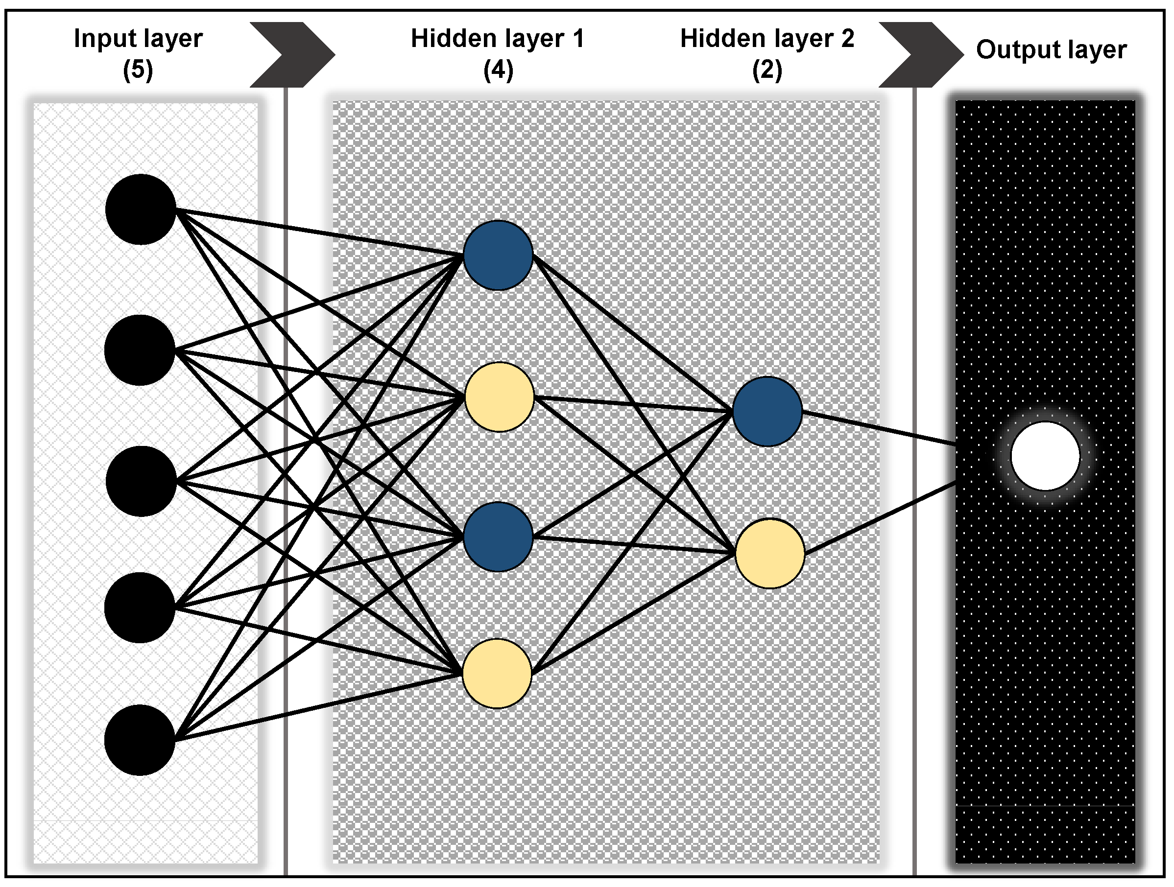
2.2.2. Multilayer Perceptron (MLP)

Multilayer perceptron or feedforward deep network is a mathematical function mapping a sort of input values to output values. According to [37], the main objective of a feedforward neural network is to approximate any function $f^{*}$, defining a mapping $y=f(x;\theta )$, and learn the value of the parameter $\theta =(w_j,v_1,\dots ,v_N)$ that makes the best function approximation.

According to [38], the MLP is given by

$$\widehat{y}=v_0+\sum _{j=1}^N{v}_{j}g\left(w_j^T{x}^{{}^{\prime }}\right)$$

(8)

where $x^{{}^{\prime }}$ is the input vector x, augmented with 1, i.e., $x^{{}^{\prime }}={(1,x^T)}^T$, $w_j$ is the weight vector for the jth hidden node, $v_0$ is the output layer intercept, $v_1,\dots ,v_N$ are the weights for the output node, $\widehat{y}$ is the network output, and g is the activation function and is used to allow a possible nonlinearity at the hidden layer. We used the logistic activation function (Equation (7)).

2.3. Mean Absolute Percentage Error (MAPE)

In this study, MAPE was used to assess the ability of models fitted and forecast the time series. The MAPE was defined by

$${\displaystyle MAPE=100\times \frac{1}{N}\sum _{i=1}^N\left|\frac{y_i-{\widehat{y}}_i}{y_i}\right|,}$$

(9)

where N is the number of fitted points, $y_i$ is the observed value, and ${\widehat{y}}_i$ is the forecast value both for instant i.

3. Results and Discussion

Figure 1a shows the behavior of electricity monthly consumption of the Brazilian industry, and the within-year variability can be seen in the yearly box-plots of Figure 1b. A greater variability can be observed in years associated with crisis, such as 2001, 2009, and 2020. In 2001, there was a crisis in the Brazilian electrical system, and in 2009, there were the consequences of the world economic crisis that started in 2008 and occurred in Brazil in 2009. The year 2020 had the greatest variability due to the COVID-19 pandemic.

For its part,

Table A1. Summary of statistical description.

Year	Mean	Variance	St. Dev.	Amplitude	Min.	Max.
1979	4616.83	70,024.88	264.62	725.00	4215.00	4940.00
1980	5123.83	65,639.24	256.20	699.00	4806.00	5505.00
1981	5095.83	11,991.61	109.51	329.00	4906.00	5235.00
1982	5324.08	74,528.27	273.00	809.00	4836.00	5645.00
1983	5669.92	142,872.81	377.99	1076.00	4994.00	6070.00
1984	6704.58	254,915.17	504.89	1578.00	5834.00	7412.00
1985	7570.00	100,401.82	316.86	890.00	7084.00	7974.00
1986	8094.83	286,936.52	535.66	1529.00	7190.00	8719.00
1987	8116.92	67,643.36	260.08	797.00	7749.00	8546.00
1988	8377.25	45,443.66	213.18	695.00	8073.00	8768.00
1989	8583.08	246,853.36	496.84	1705.00	7595.00	9300.00
1990	8322.58	262,576.99	512.42	1949.00	7145.00	9094.00
1991	8550.08	391,295.36	625.54	1814.00	7466.00	9280.00
1992	8610.58	93,964.45	306.54	1139.00	7953.00	9092.00
1993	8915.08	145,204.81	381.06	1083.00	8290.00	9373.00
1994	8921.92	136,503.90	369.46	1082.00	8368.00	9450.00
1995	9305.50	44,580.09	211.14	577.00	9070.00	9647.00
1996	9709.67	217,869.70	466.77	1637.00	8753.00	10,390.00
1997	10,143.08	185,066.81	430.19	1272.00	9455.00	10,727.00
1998	10,164.83	152,053.79	389.94	1178.00	9545.00	10,723.00
1999	10,324.33	300,464.79	548.15	1607.00	9257.00	10,864.00
2000	10,940.00	163,874.18	404.81	1398.00	10,024.00	11,422.00
2001	10,211.50	609,427.18	780.66	2160.00	9178.00	11,338.00
2002	10,635.67	247,841.33	497.84	1609.00	9431.00	11,040.00
2003	10,852.67	114,157.70	337.87	1186.00	10,345.00	11,531.00
2004	12,846.83	291,560.70	539.96	1585.00	11,829.00	13,414.00
2005	13,217.33	133,968.42	366.02	1105.00	12,496.00	13,601.00
2006	13,598.42	149,381.17	386.50	1313.00	12,851.00	14,164.00
2007	14,530.67	222,010.42	471.18	1433.00	13,592.00	15,025.00
2008	14,652.83	404,200.70	635.77	1995.00	13,417.00	15,412.00
2009	13,483.17	710,177.42	842.72	2628.00	11,924.00	14,552.00
2010	14,956.58	380,298.81	616.68	2031.00	13,425.00	15,456.00
2011	15,298.00	187,278.18	432.76	1386.00	14,467.00	15,853.00
2012	15,285.42	112,891.36	335.99	1061.00	14,567.00	15,628.00
2013	15,390.25	197,482.39	444.39	1516.00	14,370.00	15,886.00
2014	14,925.42	68,056.63	260.88	723.00	14,537.00	15,260.00
2015	14,071.50	127,615.73	357.23	1238.00	13,327.00	14,565.00
2016	13,687.75	174,712.57	417.99	1598.00	12,538.00	14,136.00
2017	13,903.92	138,837.36	372.61	1211.00	13,105.00	14,316.00
2018	14,121.92	119,368.63	345.50	1014.00	13,525.00	14,539.00
2019	13,858.17	71,473.42	267.35	864.00	13,442.00	14,306.00
2020	13,802.42	1,019,275.90	1009.59	2936.00	12,173.00	15,109.00

shows some descriptive statistics by year of the industrial electricity consumption. It can be seen in the table that there are several levels of variability in electricity consumption over the years.

Using the mean of squared errors between additive and multiplicative methods, the Holt–Winters multiplicative method obtained a better result than the additive method. Thus, it was decided to consider the multiplicative method for comparison with the other proposed models, and there is a division of the series by its seasonality component.

Then, we applied a selection algorithm to the SARIMA model that considers the candidate models through the principle of parsimony. Thus, the structure with the best result for the Akaike Information Criterion metric was the SARIMA $(1,1,1)\times {(1,1,1)}_{12}$. We considered the dynamic linear model (DLM) that captures trend and seasonality components. In this work, the dynamic regression matrix $F_t$ and the evolution matrix $G_t$ of the model are

$$\begin{array}{c}{F_t}_{1\times 13}=\left[\begin{array}{cccccc}1& 0& 1& 0& \dots & 0\end{array}\right]\hfill \end{array}$$

(10)

$$\begin{array}{c}{G_t}_{13\times 13}=\left[\begin{array}{ccccccc}1& 1& 0& 0& 0& \dots & 0\\ 0& 1& 0& 0& 0& \dots & 0\\ 0& 0& -1& -1& -1& \dots & -1\\ 0& 0& 0& 1& 0& \dots & 0\\ 0& 0& 0& 0& 1& \dots & 0\\ ⋮& ⋮& ⋮& ⋮& ⋮& \ddots & ⋮\\ 0& 0& 0& 0& 0& \dots & 1\end{array}\right].\hfill \end{array}$$

(11)

For DLM, it was assumed that the observational variance $V_t={\sigma }^2$, and the covariance matrix of the system $W_t$ is a diagonal matrix introduced by $W_t=diag({\sigma }_{\mu }^2,{\sigma }_{\beta }^2,{\sigma }_{\gamma }^2,0,0)$. These unknown variances were also estimated using Bayesian inference. Thus, to complete the specification of the model, we assumed independent inverse gamma priors distributions with means $a,a_{{\theta }_1},a_{{\theta }_2},a_{{\theta }_3}\mathrm{and}\mathrm{variances}b,b_{{\theta }_1},b_{{\theta }_2},b_{{\theta }_3},$ respectively, fixed in known values. Therefore, by using the unobservable states as latent variables, a Gibbs sampler can be run on the basis of the following full conditional densities:

$${\displaystyle \begin{array}{c}{\sigma }^2\sim IG\left(\frac{a^2}{b}+\frac{n}{2},\frac{a}{b}+\frac{1}{2}S{S}_y\right),\hfill \\ {\sigma }_{\mu }^2\sim IG\left(\frac{a_{{\theta }_1}^2}{b_{{\theta }_1}}+\frac{n}{2},\frac{a_{{\theta }_1}}{b_{{\theta }_1}}+\frac{1}{2}S{S}_{{\theta }_1}\right),\hfill \\ {\sigma }_{\beta }^2\sim IG\left(\frac{a_{{\theta }_2}^2}{b_{{\theta }_2}}+\frac{n}{2},\frac{a_{{\theta }_2}}{b_{{\theta }_2}}+\frac{1}{2}S{S}_{{\theta }_2}\right),\hfill \\ {\sigma }_{\gamma }^2\sim IG\left(\frac{a_{\theta ,3}^2}{b_{{\theta }_3}}+\frac{n}{2},\frac{a_{{\theta }_3}}{b_{{\theta }_3}}+\frac{1}{2}S{S}_{{\theta }_3}\right),\hfill \end{array}}$$

(12)

with $S{S}_y={\sum }_{t=1}^n{\left(y_t-F_t{\theta }_t\right)}^2$ and $S{S}_{{\theta }_i}={\sum }_{t=1}^T{\left({\theta }_{t,i}-{\left(G_t{\theta }_{t-1}\right)}_i\right)}^2$, for $i=1,2,3$. The full conditional density of the states is a normal distribution, and it is covered in the used dlm package [39].

Regarding the approach of artificial neural networks, the applied NNAR model has the results as an average of 20 networks, each of which is a NNAR(2,2,1) with nine weights. We also considered an MLP model with five nodes in the input layer, four nodes in the first hidden layer, two nodes in the second hidden layer, and one node in the output layer (Figure 2).

In that sense, Figure 3 presents the fitted results for all models considered. The models are able to fit the observed data even in periods of economic crisis. It can be seen in this figure that the models are able to capture the behavior of the time series of industrial electricity consumption.

Indeed, Figure 4 shows the forecasting results for the models under consideration. It can be seen in the figure that the models were unable to give an accurate forecast for the months of April, May, and June of 2020. The electricity consumption in these months was impacted by the COVID-19 pandemic. This period marked the beginning of the pandemic in Brazil.

From this perspective,

Table 2. Mean absolute percentage error for the six models under consideration for model fit and model forecasting considering the training and testing data, respectively.

Model	Fitted	Forecast
Holt–Winters	2.51	4.09
SARIMA	1.88	6.17
TBATS	1.99	3.77
DLM	1.87	4.09
NNAR	2.40	4.77
MLP	1.48	3.41

shows the mean absolute percentage errors (MAPE) for all models considering the training and testing data of the industrial electricity consumption time series. The MLP model provided the best MAPE results for the training data (or model fit) and test data (or forecasting). The fitted models to electricity consumption data provided a percent mean square error of less than $2.5\%$.

Finally,

Table 3. Mean absolute percentage error, considering the six models, for $h=1,\dots ,24$ steps-ahead out-of-sample forecasts applied to the electricity consumption of the Brazilian industry.

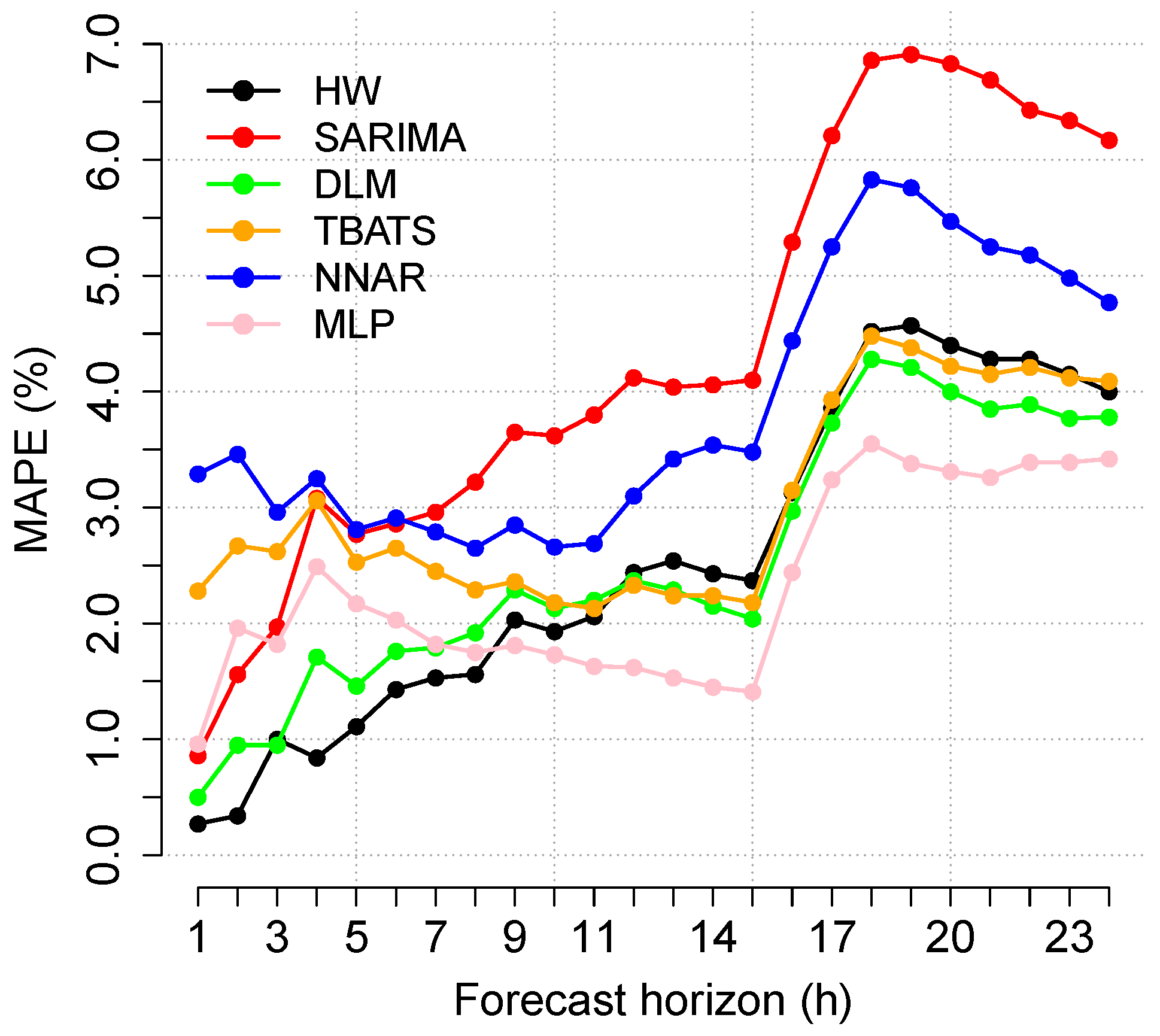
Step	HW	SARIMA	TBATS	DLM	NNAR	MLP
1	0.27	0.86	0.50	2.28	3.29	0.96
2	0.34	1.56	0.95	2.67	3.46	1.96
3	1.00	1.97	0.95	2.62	2.96	1.82
4	0.84	3.08	1.71	3.06	3.25	2.49
5	1.11	2.77	1.46	2.53	2.81	2.17
6	1.43	2.86	1.76	2.65	2.91	2.03
7	1.53	2.96	1.79	2.45	2.79	1.82
8	1.56	3.22	1.92	2.29	2.65	1.75
9	2.03	3.65	2.29	2.36	2.85	1.81
10	1.93	3.62	2.13	2.18	2.66	1.73
11	2.06	3.80	2.20	2.13	2.69	1.63
12	2.44	4.12	2.37	2.33	3.10	1.62
13	2.54	4.04	2.29	2.24	3.42	1.53
14	2.43	4.06	2.15	2.24	3.54	1.45
15	2.37	4.10	2.04	2.18	3.48	1.41
16	3.13	5.29	2.97	3.15	4.44	2.44
17	3.86	6.21	3.73	3.93	5.25	3.24
18	4.52	6.86	4.28	4.48	5.83	3.55
19	4.57	6.91	4.21	4.38	5.76	3.38
20	4.40	6.83	4.00	4.22	5.47	3.31
21	4.28	6.69	3.85	4.15	5.25	3.26
22	4.28	6.43	3.89	4.21	5.18	3.39
23	4.15	6.34	3.77	4.12	4.98	3.39
24	4.00	6.17	3.78	4.09	4.77	3.42
Average	2.54	4.35	2.54	3.04	3.87	2.32

gives the MAPE for each forecast horizon yielded by all models under consideration. In this step, the fitted models were used to obtain the forecast up to h steps ahead $(h=1,2,3,\dots ,24)$, and then, the MAPE was calculated for each forecast horizon. The bold entries identify the model that performs best for the corresponding level and forecast horizon, based on the smallest value of MAPE. The last row presents the average MAPE considering all forecast horizons. It can be seen in the table that the Holt–Winters model presented better results for MAPE up to the horizon of eight steps ahead, with the exception of the horizon of three steps ahead, in which the TBATS model resulted in a better result. However, from the horizon of nine steps ahead, the MLP model presented the best results for the MAPE. The MLP model presented the best average MAPE among all the models considered.

To complement Table 3, Figure 5 shows the behavior of MAPE for the forecast horizon of all six models considered in this study. It can be seen in this figure that all models showed a significant increase in the MAPE values after the forecast horizon of 16 steps ahead. This increase can be associated to the beginning of the COVID-19 pandemic in Brazil. Another relevant feature of this figure was the decrease of the MAPE after July 2020 for all models.

4. Conclusions

The exercise of forecasting the industry’s electricity consumption is essential for energy planning in a given country or region. In this way, this study applied time-series forecasting models (statistical approaches and artificial neural network approaches) to the industrial electricity consumption in the Brazilian system.

The results of the study indicate the following: (i) the models considered have a satisfactory ability to adjust to the data; (ii) the models managed to capture the complex structure of the data involving the crises (peaks in the series) in the years 2001 and 2009; and (iii) the MLP model presented the best predictive capacity for the group of proposed models, among which the Holt–Winters method was the overall best for short-term forecasting. In addition, the results found are useful as instruments to support decision making by economic agents and legislators of the Brazilian energy system.

For future research, we can apply other univariate models, such as Recurrent Neural Network (RNN), Long Short-Term Memory (LSTM) [40,41], and bootstrap-based models, and develop a hierarchical time-series forecast strategy to compare with the classical structure applied in this study. Finally, another avenue for future work would be to study the multivariate models (such as vector autoregressive, Bayesian vector autoregressive, artificial neural networks models with multiple features in the input layer) and compare with the univariate approach.

References

- Silva, F.L.C.; Souza, R.C.; Oliveira, F.L.C.; Lourenco, P.M.; Calili, R.F. A bottom-up methodology for long term electricity consumption forecasting of an industrial sector—Application to pulp and paper sector in Brazil. Energy 2018, 144, 1107–1118. [Google Scholar] [CrossRef]
- López-Gonzales, J.L.; Castro Souza, R.; Leite Coelho da Silva, F.; Carbo-Bustinza, N.; Ibacache-Pulgar, G.; Calili, R.F. Simulation of the Energy Efficiency Auction Prices via the Markov Chain Monte Carlo Method. Energies 2020, 13, 4544. [Google Scholar] [CrossRef]
- Ardakani, F.J.; Ardehali, M.M. Novel effects of demand side management data on accuracy of electrical energy consumption modeling and long-term forecasting. Energy Convers. Manag. 2014, 78, 745–752. [Google Scholar] [CrossRef]
- Taylor, J.W.; Buizza, R. Using weather ensemble predictions in electricity demand forecasting. Int. J. Forecast. 2003, 19, 57–70. [Google Scholar] [CrossRef]
- Bianco, V.; Manca, O.; Nardini, S. Electricity consumption forecasting in italy using linear regression models. Energy 2009, 34, 1413–1421. [Google Scholar] [CrossRef]
- Taylor, J.; Mcsharry, P. Short-term load forecasting methods: An evaluation based on european data. Power Syst. IEEE Trans. 2007, 22, 2213–2219. [Google Scholar] [CrossRef] [Green Version]
- Santana, A.L.; Conde, G.B.; Rego, L.P.; Rocha, C.A.; Cardoso, D.L.; Costa, J.C.; Bezerra, U.H.; Francs, C.R. Predict decision support system for load forecasting and inference: A new undertaking for brazilian power suppliers. Electr. Power Energy Syst. 2012, 38, 33–45. [Google Scholar] [CrossRef]
- Sadownik, R.; Barbosa, E.P. Short term forecasting of industrial electricity consumption in brazil. J. Forecast. 1999, 18, 215–224. [Google Scholar] [CrossRef]
- Fan, S.; Hyndman, R.J. Short-term load forecasting based on a semi-parametric additive model. IEEE Trans. Power Syst. 2012, 27, 134–141. [Google Scholar] [CrossRef] [Green Version]
- Huang, Y.-H.; Chang, Y.-L.; Fleiter, T. A critical analysis of energy efficiency improvement potentials in taiwan’s cement industry. Energy Policy 2016, 96, 14–26. Available online: https://www.journals.elsevier.com/energy-policy (accessed on 25 November 2021). [CrossRef]
- Silva, F.L.; Oliveira, F.L.; Souza, R.C. A bottom-up bayesian extension for long term electricity consumption forecasting. Energy 2019, 167, 198–210. [Google Scholar] [CrossRef]
- Martínez-Álvarez, F.; Troncoso, A.; Asencio-Cortés, G.; Riquelme, J.C. A Survey on Data Mining Techniques Applied to Electricity-Related Time Series Forecasting. Energies 2015, 8, 13162–13193. [Google Scholar] [CrossRef] [Green Version]
- Divina, F.; García Torres, M.; Goméz Vela, F.A.; Vázquez Noguera, J.L. A Comparative Study of Time Series Forecasting Methods for Short Term Electric Energy Consumption Prediction in Smart Buildings. Energies 2019, 12, 1934. [Google Scholar] [CrossRef] [Green Version]
- Ramos, D.; Faria, P.; Vale, Z.; Mourinho, J.; Correia, R. Industrial Facility Electricity Consumption Forecast Using Artificial Neural Networks and Incremental Learning. Energies 2020, 13, 4774. [Google Scholar] [CrossRef]
- Rocha, H.R.; Honorato, I.H.; Fiorotti, R.; Celeste, W.C.; Silvestre, L.J.; Silva, J.A. An Artificial Intelligence based scheduling algorithm for demand-side energy management in Smart Homes. Appl. Energy 2021, 282, 116–145. [Google Scholar] [CrossRef]
- Sulandari, W.; Subanar, S.; Lee, M.H.; Rodrigues, P.C. Time series forecasting using singular spectrum analysis, fuzzy systems and neural networks. MethodsX 2020, 7, 101015. [Google Scholar] [CrossRef] [PubMed]
- Sulandari, W.; Subanar, S.; Suhartono, S.; Utami, H.; Lee, M.H.; Rodrigues, P.C. SSA-based hybrid forecasting models and applications. Bull. Electr. Eng. Inform. 2020, 9, 2178–2188. [Google Scholar] [CrossRef]
- Sulandari, W.; Lee, M.H.; Rodrigues, P.C. Indonesian electricity load forecasting using singular spectrum analysis, fuzzy systems and neural networks. Energy 2020, 190, 116408. [Google Scholar] [CrossRef]
- Makridakis, S.; Hibon, M. The m3-competition: Results, conclusions and implications. Int. J. Forecast. 2000, 16, 451–476. [Google Scholar] [CrossRef]
- Makridakis, S.; Spiliotis, E.; Assimakopoulos, V.; Chen, Z.; Gaba, A.; Tsetlin, I.; Winkler, R. The m5 Uncertainty Competition: Results, Findings and Conclusions. 2020. Available online: https://www.researchgate.net/publication/346493740_The_M5_Uncertainty_competition_Results_findings_and_conclusions (accessed on 15 November 2021).
- Makridakis, S.; Fry, C.; Petropoulos, F.; Spiliotis, E. The Future of Forecasting Competitions: Design Attributes and Principles. 2021. Available online: https://arxiv.org/abs/2102.04879 (accessed on 1 November 2021).
- Du Preez, J.; Witt, S. Univariate versus multivariate time series forecasting: An application to international tourism demand. Int. J. Forecast. 2003, 19, 435–451. Available online: https://www.sciencedirect.com/science/article/pii/S0169207002000572 (accessed on 1 December 2021). [CrossRef]
- Todorov, H.; Searle-White, E.; Gerber, S. Applying univariate vs. multivariate statistics to investigate therapeutic efficacy in (pre)clinical trials: A Monte Carlo simulation study on the example of a controlled preclinical neurotrauma trial. PLoS ONE 2020, 15, 798. [Google Scholar] [CrossRef]
- Rana, M.; Koprinska, I.; Agelidis, V. Univariate and multivariate methods for very short-term solar photovoltaic power forecasting. Energy Convers. Manag. 2021, 121, 380–390. Available online: https://www.sciencedirect.com/science/article/pii/S0196890416303934 (accessed on 2 December 2021). [CrossRef]
- Ivanova, M.; Herron, T.; Dronkers, N.; Baldo, J. An empirical comparison of univariate versus multivariate methods for the analysis of brain–behavior mapping. Hum. Brain Mapp. 2021, 42, 1070–1101. Available online: https://onlinelibrary.wiley.com/doi/abs/10.1002/hbm.25278 (accessed on 4 December 2021). [CrossRef] [PubMed]
- Lütkepohl, H. Introduction to Multiple Time Series Analysis; Springer Science & Business Media: Berlin/Heidelberg, Germany, 2013. [Google Scholar]
- Central Bank of Brazil. Time Series Management System—v2.1. 2021. Available online: https://www3.bcb.gov.br/sgspub/localizarseries/localizarSeries.do?method=prepararTelaLocalizarSeries (accessed on 10 November 2021).
- R Core Team. R: A Language and Environment for Statistical Computing; R Foundation for Statistical Computing: Vienna, Austria, 2021; Available online: https://www.R-project.org/ (accessed on 9 November 2021).
- Holt, C.C. Forecasting seasonals and trends by exponentially weighted moving averages. Int. J. Forecast. 1957, 20, 5–10. [Google Scholar] [CrossRef]
- Winters, P.R. Forecasting sales by exponentially weighted moving averages. Manag. Sci. 1960, 6, 324–342. [Google Scholar] [CrossRef]
- Box, G.E.P.; Jenkins, G.M.; Reinsel, G.C.; Ljung, G.M. Time Series Analysis: Forecasting and Control; Wiley: Hoboken, NJ, USA, 2015. [Google Scholar]
- West, M.; Harrison, J. Bayesian Forecasting and Dynamic Models; Springer Science & Business Media: Berlin/Heidelberg, Germany, 2006. [Google Scholar]
- Livera, A.M.D.; Hyndman, R.J.; Snyder, R.D. Forecasting time series with complex seasonal patterns using exponential smoothing. J. Am. Stat. Assoc. 2011, 106, 1513–1527. [Google Scholar] [CrossRef] [Green Version]
- Hyndman, R.J.; Athanasopoulos, G. Forecasting: Principles and Practice; OTexts: Melbourne, Australia, 2018. [Google Scholar]
- Veloz, A.; Salas, R.; Allende-Cid, H.; Allende, H.; Moraga, C. Identification of lags in nonlinear autoregressive time series using a flexible fuzzy model. Neural Process. Lett. 2016, 43, 641–666. [Google Scholar] [CrossRef]
- Hyndman, R.; Athanasopoulos, G.; Bergmeir, C.; Caceres, G.; Chhay, L.; O’Hara-Wild, M.; Petropoulos, F.; Razbash, S.; Wang, E.; Yasmeen, F. Forecast: Forecasting Functions for Time Series and Linear Models. R Package Version 8.15. 2021. Available online: https://pkg.robjhyndman.com/forecast/ (accessed on 10 November 2021).
- Goodfellow, I.; Bengio, Y.; Courville, A. Deep Learning; MIT Press: Cambridge, MA, USA, 2016. [Google Scholar]
- Ahmed, N.K.; Atiya, A.F.; Gayar, N.E.; El-Shishiny, H.E. An Empirical Comparison of Machine Learning Models for Time Series Forecasting. Econom. Rev. 2010, 29, 594–621. [Google Scholar] [CrossRef]
- Petris, G. An R Package for Dynamic Linear Models. J. Stat. Softw. Artic. 2020, 36, 1–16. Available online: https://www.jstatsoft.org/v036/i12 (accessed on 3 November 2021).
- Vivas, E.; Allende-Cid, H.; Salas, R. A systematic review of statistical and machine learning methods for electrical power forecasting with reported mape score. Entropy 2020, 22, 1412. [Google Scholar] [CrossRef] [PubMed]
- Cordova, C.H.; Portocarrero, M.N.L.; Salas, R.; Torres, R.; Rodrigues, P.C.; López-Gonzales, J.L. Air quality assessment and pollution forecasting using artificial neural networks in Metropolitan Lima-Peru. Sci. Rep. 2021, 11, 24232. [Google Scholar] [CrossRef] [PubMed]