Use of Artificial Neural Networks to Predict Fuel Consumption on the Basis of Technical Parameters of Vehicles
Abstract
1. Introduction
2. Materials and Methods
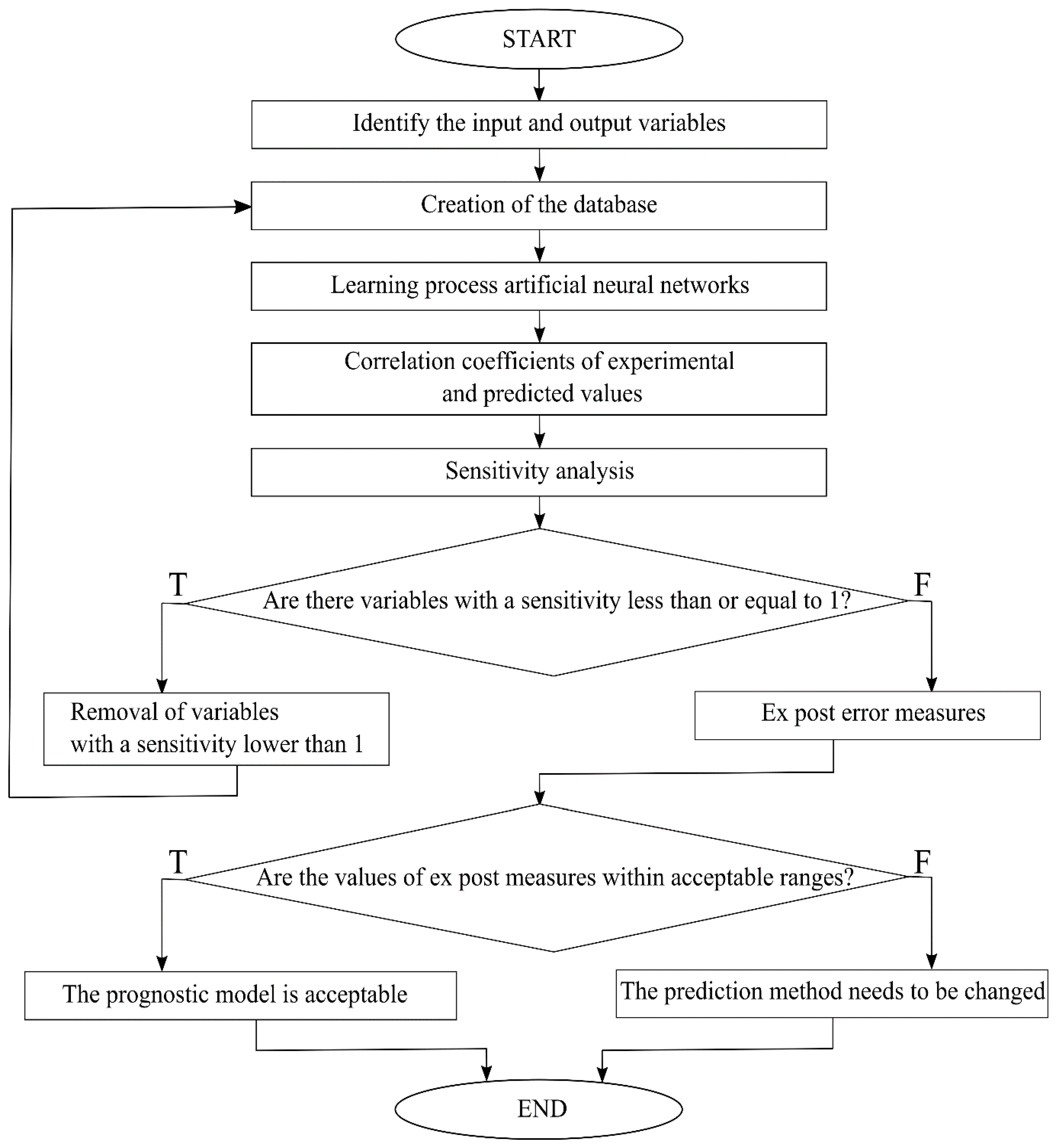
- Selecting the technical parameters having a significant impact on the quantity of fuel consumption;
- Developing a database for the neural network learning process;
- Creating a set of neural networks and selecting the best of them;
- Calculating a correlation and determining the coefficients and carrying out a sensitivity analysis in respect of the input variables;
- Making an attempt to simplify the predictive model—an elimination of the input variables for which the sensitivity coefficient takes values less than or is equal to 1.0;
- Creating a new set of neural networks from a reduced database and selecting the best of them;
- Calculating the correlation and determining the coefficients, as well as performing a sensitivity analysis of the input variables for the reduced model;
- Comparing and evaluating an acceptability of the predictive models on the basis of the values of the ex post prediction error measures.
2.1. Identification of the Input and Output Variables
2.2. Correlation Coefficients
2.3. Sensitivity Analysis
2.4. Prediction Errors
- Mean squared error (MSE):
- Root mean squared error (RMSE):
- Mean absolute percentage error (MAPE):
2.5. Database
3. Results
3.1. ANN Model with 12 Input Variables
3.2. ANN Model with 11 Input Variables
4. Discussion
5. Conclusions
Author Contributions
Funding
Institutional Review Board Statement
Informed Consent Statement
Data Availability Statement
Acknowledgments
Conflicts of Interest
Appendix A
| Input Layer | Hidden Layer | |||||||||
|---|---|---|---|---|---|---|---|---|---|---|
| 1 | 2 | 3 | 4 | 5 | 6 | 7 | 8 | 9 | 10 | |
| 1 (DE) | −1.6702 | −0.4328 | −0.7698 | 0.8842 | −1.3829 | −0.9280 | −0.6757 | −1.7382 | −0.6358 | −1.3018 |
| 2 (NC) | −0.2134 | −0.2676 | −0.5045 | −0.7850 | −0.3062 | −0.8504 | 0.1644 | −0.6858 | −0.2788 | −0.0615 |
| 3 (NV) | 0.5032 | 0.8776 | 0.4737 | 0.3170 | −0.7939 | 0.3828 | −0.8991 | 0.1832 | 0.1462 | 1.1559 |
| 4 (PMAX) | −0.5863 | 0.1890 | 0.6193 | −1.6520 | −1.0632 | −2.2077 | −0.7404 | 0.8146 | −0.4640 | −0.3713 |
| 5 (TMAX) | −0.0449 | 0.7842 | 0.2105 | 1.1824 | −0.9961 | 0.4626 | −0.1905 | 0.2780 | 0.6646 | 0.1408 |
| 6 (CR) | −0.0791 | 0.0734 | 0.0366 | 0.3923 | 1.0082 | 2.2354 | 0.6899 | −0.1457 | 0.8236 | 0.4095 |
| 7 (WV) | −0.1617 | −1.7266 | −0.6313 | −0.9371 | −0.6737 | −0.0869 | −0.1681 | −0.3257 | −0.0566 | −0.9544 |
| 8 (ET1) | −0.6947 | −0.0671 | −0.2853 | 0.9236 | −0.1842 | −0.0345 | −0.2660 | 0.2771 | −0.3976 | −0.6242 |
| 9 (ET2) | −0.6880 | −0.0323 | −0.1665 | 0.3564 | 0.2925 | −0.0290 | 0.4719 | −0.8035 | −0.4205 | −0.0219 |
| 10 (ET3) | 0.6815 | −0.1030 | 0.4876 | −1.5242 | 0.3250 | 0.2675 | −0.2736 | 0.3837 | 0.4258 | 0.3578 |
| 11 (ET4) | 0.5295 | 0.4399 | 0.2030 | −0.0720 | 0.2472 | 0.1064 | 0.3583 | 0.3559 | 0.2763 | 0.6396 |
| 12 (FI1) | −0.0227 | 0.2997 | 0.0685 | −0.8359 | 0.6512 | −0.1770 | 0.4561 | 1.1345 | −0.7756 | −0.1540 |
| 13 (FI2) | −0.1239 | −0.0892 | 0.1578 | 0.4585 | 0.0713 | 0.4177 | −0.1588 | −0.8407 | 0.6401 | 0.4933 |
| 14 (BT1) | −0.2002 | 0.1789 | 0.8938 | −0.4311 | −0.5010 | −0.4624 | −1.0636 | 0.3441 | −0.1712 | 0.0991 |
| 15 (BT2) | −0.0327 | 0.0590 | −0.3720 | 0.1708 | 0.9242 | 0.5391 | 0.2677 | −0.0638 | 0.0356 | 0.0960 |
| 16 (BT3) | 0.2697 | −0.1014 | −0.3337 | 0.1720 | −0.0261 | 0.7786 | 0.5561 | −0.0178 | 0.1086 | 0.3105 |
| 17 (BT4) | −0.1344 | 0.1468 | 0.0944 | −0.2452 | 0.3221 | −0.5298 | 0.4897 | −0.0211 | −0.0674 | −0.1185 |
| 18 (TG1) | 0.5821 | 0.1392 | −0.1230 | −0.3436 | 0.2794 | 0.1048 | −0.0507 | 0.1859 | −0.0826 | 0.4532 |
| 19 (TG2) | −0.7316 | 0.1256 | 0.4036 | −0.0241 | 0.4630 | 0.2031 | 0.3125 | 0.0607 | −0.0714 | −0.1088 |
| 20 (DT1) | 0.2578 | 0.0524 | 0.0842 | −0.1878 | 0.2959 | 0.0029 | −0.0104 | 0.1082 | −0.1622 | 0.1625 |
| 21 (DT2) | 0.1273 | 0.0253 | 0.2565 | −0.0907 | 0.4757 | 0.1312 | 0.2240 | −0.1555 | −0.0889 | −0.0081 |
| 22 (DT3) | −0.5231 | 0.1135 | −0.0467 | −0.1013 | −0.0940 | 0.1615 | 0.0536 | 0.3091 | 0.1611 | 0.1881 |
| Bias | −0.1355 | 0.2605 | 0.2510 | −0.3920 | 0.6944 | 0.2470 | 0.2161 | 0.2704 | −0.1449 | 0.3282 |
| Hidden Layer | Output Layer | ||
|---|---|---|---|
| 1 (FCU) | 2 (FCH) | 3 (FCM) | |
| 1 | −1.1765 | −1.1077 | −0.9716 |
| 2 | 0.2570 | −0.3898 | −0.0372 |
| 3 | −0.4454 | −0.3606 | −0.3983 |
| 4 | −0.8704 | −0.8448 | −0.8939 |
| 5 | −0.1054 | −0.0468 | −0.0825 |
| 6 | 0.2102 | 0.1440 | 0.1772 |
| 7 | −0.5770 | −0.6157 | −0.5815 |
| 8 | −0.2557 | −0.0877 | −0.1866 |
| 9 | −1.1079 | −0.1888 | −0.6022 |
| 10 | −0.4194 | −0.4122 | −0.4607 |
| Bias | 3.0602 | 2.3757 | 2.7454 |
Appendix B
| Input Layer | Hidden Layer | |||||||||
|---|---|---|---|---|---|---|---|---|---|---|
| 1 | 2 | 3 | 4 | 5 | 6 | 7 | 8 | 9 | 10 | |
| 1 (DE) | −1.6639 | −0.5427 | −0.6400 | −2.2715 | −0.3293 | −0.0143 | −1.4225 | 0.3937 | −0.2811 | −0.8970 |
| 2 (NC) | −0.5674 | −1.0048 | −0.2679 | 0.0996 | −0.0824 | −0.6307 | −0.7623 | −0.6331 | −0.4103 | 0.3619 |
| 3 (NV) | 0.5247 | 0.0188 | 0.4472 | −0.5617 | −0.0305 | 0.6609 | 0.4463 | 0.3168 | 0.5853 | −1.1059 |
| 4 (PMAX) | 0.0755 | −1.8274 | 0.1991 | −0.3889 | −0.3997 | −0.3760 | 0.8215 | −1.1011 | −0.4183 | −2.1368 |
| 5 (TMAX) | 0.6920 | 0.3141 | 0.4897 | 0.4168 | 0.1669 | 0.2526 | −0.0058 | 0.7507 | 0.1781 | −0.9557 |
| 6 (CR) | 0.0159 | 2.7565 | 0.2241 | 0.3183 | 1.0543 | 0.3537 | 0.3164 | 0.3963 | 0.6138 | 0.3405 |
| 7 (WV) | −0.0144 | 0.6246 | −1.0896 | 0.0063 | 0.0568 | −1.1912 | −0.6269 | −0.4642 | −0.5363 | −0.6934 |
| 8 (ET1) | −0.2732 | 0.0431 | −0.2841 | −0.1888 | −0.6847 | −0.0800 | −0.5504 | 0.4216 | −0.4343 | −0.2838 |
| 9 (ET2) | −0.3391 | −0.2746 | −0.1935 | −0.3192 | −0.4043 | 0.0845 | 0.6315 | −0.0058 | −0.1987 | 0.3312 |
| 10 (ET3) | 0.5250 | −0.0607 | 0.4576 | 0.1264 | 0.4614 | −0.5007 | −0.1404 | −0.7093 | 0.4074 | −0.2256 |
| 11 (ET4) | 0.5208 | −0.0179 | 0.6684 | 0.6342 | 0.1560 | 0.3443 | 0.4633 | 0.0942 | 0.0905 | 0.1696 |
| 12 (FI1) | 0.4634 | −0.3963 | 0.5690 | 0.7061 | −1.4592 | −0.2166 | 0.6892 | −1.1845 | −0.3073 | −0.4728 |
| 13 (FI2) | −0.0400 | 0.0486 | 0.1505 | −0.4326 | 1.0319 | 0.1433 | −0.3477 | 1.0755 | 0.2147 | 0.4304 |
| 14 (BT1) | 0.6902 | −0.1546 | 0.5649 | −0.4344 | 0.0590 | −0.2584 | 0.4335 | −0.5813 | 0.5127 | −1.0058 |
| 15 (BT2) | −0.0610 | 0.1546 | 0.2930 | 0.1795 | −0.2164 | −0.0684 | −0.1197 | 0.2826 | −0.3488 | 0.5950 |
| 16 (BT3) | −0.0225 | 0.1974 | −0.2008 | 0.3968 | −0.2358 | 0.1029 | −0.0708 | 0.3280 | −0.1172 | 0.1952 |
| 17 (BT4) | −0.1676 | −0.5538 | 0.0276 | 0.1746 | 0.0369 | 0.0677 | 0.1575 | −0.1782 | −0.0472 | 0.1863 |
| 18 (DT1) | 0.1071 | −0.2094 | 0.1963 | 0.3067 | −0.2461 | −0.1187 | −0.1024 | −0.2039 | 0.0837 | 0.4892 |
| 19 (DT2) | −0.1270 | 0.1834 | 0.0999 | −0.1648 | 0.0187 | 0.0880 | 0.3178 | −0.0097 | 0.1443 | 0.7366 |
| 20 (DT3) | 0.5048 | −0.3027 | 0.3703 | 0.1241 | −0.1429 | −0.0232 | 0.1458 | 0.0309 | −0.2511 | −1.2196 |
| Bias | 0.4652 | −0.3830 | 0.7129 | 0.2545 | −0.3994 | −0.1438 | 0.3726 | −0.1437 | −0.1077 | −0.0582 |
| Hidden Layer | Output Layer | ||
|---|---|---|---|
| 1 (FCU) | 2 (FCH) | 3 (FCM) | |
| 1 | −0.0978 | 0.1020 | −0.0372 |
| 2 | 0.5263 | 0.3501 | 0.4651 |
| 3 | −0.0622 | −0.2329 | −0.1141 |
| 4 | −0.9635 | −0.5855 | −0.7522 |
| 5 | −0.7370 | −0.0164 | −0.4454 |
| 6 | 0.5206 | −1.2625 | −0.7602 |
| 7 | −0.6456 | −0.3207 | −0.4459 |
| 8 | −0.4761 | −0.2743 | −0.3227 |
| 9 | −1.1609 | −1.1352 | −1.0552 |
| 10 | −0.3650 | −0.3047 | −0.3596 |
| Bias | 2.6763 | 2.0268 | 2.3380 |
References
- Zhu, D.; Zheng, X. Fuel Consumption and Emission Characteristics in Asymmetric Twin-Scroll Turbocharged Diesel Engine with Two Exhaust Gas Recirculation Circuits. Appl. Energy 2019, 238, 985–995. [Google Scholar] [CrossRef]
- Asher, Z.D.; Galang, A.A.; Briggs, W.; Johnston, B.; Bradley, T.H.; Jathar, S. Economic and Efficient Hybrid Vehicle Fuel Economy and Emissions Modeling Using an Artificial Neural Network; SAE Technical Paper 2018-01-0315; SAE: Warrenville, PA, USA, 2018; pp. 1–8. [Google Scholar] [CrossRef]
- Wang, J.; Rakha, H.A. Fuel Consumption Model for Conventional Diesel Buses. Appl. Energy 2016, 170, 394–402. [Google Scholar] [CrossRef]
- Zhang, Z.; Wei, L.; Lim, A. An Evolutionary Local Search for the Capacitated Vehicle Routing Problem Minimizing Fuel Consumption under Three-Dimensional Loading Constraints. Transp. Res. Part B Methodol. 2015, 82, 20–35. [Google Scholar] [CrossRef]
- Macharis, C.; Van Hoeck, E.; Pekin, E.; van Lier, T. A Decision Analysis Framework for Intermodal Transport: Comparing Fuel Price Increases and the Internalisation of External Costs. Transp. Res. Part A Policy Pract. 2010, 44, 550–561. [Google Scholar] [CrossRef]
- Elaiw, A.M.; Xia, X.; Shehata, A.M. Minimization of Fuel Costs and Gaseous Emissions of Electric Power Generation by Model Predictive Control. Math. Probl. Eng. 2013, 2013, 1–15. [Google Scholar] [CrossRef][Green Version]
- Lo, C.-L.; Chen, C.-H.; Kuan, T.-S.; Lo, K.-R.; Cho, H.-J. Fuel Consumption Estimation System and Method with Lower Cost. Symmetry 2017, 9, 105. [Google Scholar] [CrossRef]
- Zargarnezhad, S.; Dashti, R.; Ahmadi, R. Predicting Vehicle Fuel Consumption in Energy Distribution Companies Using ANNs. Transp. Res. Part D Transp. Environ. 2019, 74, 174–188. [Google Scholar] [CrossRef]
- Lasocki, J.; Boguszewski, K. Environmental Effects of Driving Style: Impact on Fuel Consumption. E3s Web Conf. 2019, 100, 8. [Google Scholar] [CrossRef]
- Nutramon, T.; Supachart, C. Influence of Driving Cycles on Exhaust Emissions and Fuel Consumption of Gasoline Passenger Car in Bangkok. J. Environ. Sci. 2009, 21, 604–611. [Google Scholar] [CrossRef]
- Wu, X.; Freese, D.; Cabrera, A.; Kitch, W.A. Electric Vehicles’ Energy Consumption Measurement and Estimation. Transp. Res. Part D Transp. Environ. 2015, 34, 52–67. [Google Scholar] [CrossRef]
- Yang, Z.; Liu, Y.; Wu, L.; Martinet, S.; Zhang, Y.; Andre, M.; Mao, H. Real-World Gaseous Emission Characteristics of Euro 6b Light-Duty Gasoline- and Diesel-Fueled Vehicles. Transp. Res. Part D Transp. Environ. 2020, 78, 1–11. [Google Scholar] [CrossRef]
- Zamboni, G.; Moggia, S.; Capobianco, M. Hybrid EGR and Turbocharging Systems Control for Low NO and Fuel Consumption in an Automotive Diesel Engine. Appl. Energy 2016, 165, 839–848. [Google Scholar] [CrossRef]
- D’Ambrosio, S.; Ferrari, A. Diesel Engines Equipped with Piezoelectric and Solenoid Injectors: Hydraulic Performance of the Injectors and Comparison of the Emissions, Noise and Fuel Consumption. Appl. Energy 2018, 211, 1324–1342. [Google Scholar] [CrossRef]
- Galloni, E.; Fontana, G.; Palmaccio, R. Effects of Exhaust Gas Recycle in a Downsized Gasoline Engine. Appl. Energy 2013, 105, 99–107. [Google Scholar] [CrossRef]
- Mao, B.; Yao, M.; Zheng, Z.; Liu, H. Effects of Dual Loop EGR and Variable Geometry Turbocharger on Performance and Emissions of a Diesel Engine; SAE International: Warrendale, PA, USA, 2016. [Google Scholar]
- Dey, S.; Kamlu, S.; Mishra, S.K. Optimization of Fuel Consumption and Emission for Hybrid Electric Vehicle. Adv. Intell. Syst. Comput. 2016, 394, 715–722. [Google Scholar] [CrossRef]
- Rakopoulos, C.D.; Antonopoulos, K.A.; Rakopoulos, D.C.; Hountalas, D.T.; Giakoumis, E.G. Comparative Performance and Emissions Study of a Direct Injection Diesel Engine Using Blends of Diesel Fuel with Vegetable Oils or Bio-Diesels of Various Origins. Energy Convers. Manag. 2006, 47, 3272–3287. [Google Scholar] [CrossRef]
- Yao, Y.; Zhao, X.; Zhang, Y.; Chen, C.; Rong, J. Modeling of Individual Vehicle Safety and Fuel Consumption under Comprehensive External Conditions. Transp. Res. Part D Transp. Environ. 2020, 79. [Google Scholar] [CrossRef]
- Typaldos, P.; Papamichail, I.; Papageorgiou, M. Minimization of Fuel Consumption for Vehicle Trajectories. IEEE Trans. Intell. Transp. Syst. 2020, 21, 1716–1727. [Google Scholar] [CrossRef]
- Khan, W.A.; Chung, S.-H.; Ma, H.-L.; Liu, S.Q.; Chan, C.Y. A Novel Self-Organizing Constructive Neural Network for Estimating Aircraft Trip Fuel Consumption. Transp. Res. Part E Logist. Transp. Rev. 2019, 132, 72–96. [Google Scholar] [CrossRef]
- Tarelko, W.; Rudzki, K. Applying Artificial Neural Networks for Modelling Ship Speed and Fuel Consumption. Neural Comput. Applic. 2020, 32, 17379–17395. [Google Scholar] [CrossRef]
- Le, L.T.; Lee, G.; Park, K.-S.; Kim, H. Neural Network-Based Fuel Consumption Estimation for Container Ships in Korea. Marit. Policy Manag. 2020, 47, 615–632. [Google Scholar] [CrossRef]
- Gkerekos, C.; Lazakis, I.; Theotokatos, G. Machine Learning Models for Predicting Ship Main Engine Fuel Oil Consumption: A Comparative Study. Ocean Eng. 2019, 188, 106282. [Google Scholar] [CrossRef]
- Jeon, M.; Noh, Y.; Shin, Y.; Lim, O.-K.; Lee, I.; Cho, D. Prediction of Ship Fuel Consumption by Using an Artificial Neural Network. J. Mech. Sci. Technol. 2018, 32, 5785–5796. [Google Scholar] [CrossRef]
- Kee, K.-K.; Lau Simon, B.-Y.; Yong Renco, K.-H. Artificial Neural Network Back-Propagation Based Decision Support System for Ship Fuel Consumption Prediction. In Proceedings of the 5th IET International Conference on Clean Energy and Technology (CEAT2018), Kuala Lumpur, Malaysia, 5–6 September 2018; Volume 2018. [Google Scholar]
- Du, Y.; Meng, Q.; Wang, S.; Kuang, H. Two-Phase Optimal Solutions for Ship Speed and Trim Optimization over a Voyage Using Voyage Report Data. Transp. Res. Part B Methodol. 2019, 122, 88–114. [Google Scholar] [CrossRef]
- Siami-Irdemoosa, E.; Dindarloo, S.R. Prediction of Fuel Consumption of Mining Dump Trucks: A Neural Networks Approach. Appl. Energy 2015, 151, 77–84. [Google Scholar] [CrossRef]
- Borges, P.H.M.; Mendoza, Z.M.S.H.; Maia, J.C.S.; Bianchini, A.; Fernándes, H.C. Estimation of Fuel Consumption in Agricultural Mechanized Operations Using Artificial Neural Networks. Eng. Agríc. 2017, 37, 136–147. [Google Scholar] [CrossRef][Green Version]
- Wysocki, O.; Deka, L.; Elizondo, D.; Kropiwnicki, J.; Czyżewicz, J. Heavy Duty Vehicle Fuel Consumption Modelling Based on Exploitation Data by Using Artificial Neural Networks. In Advances in Computational Intelligence; Rojas, I., Joya, G., Catala, A., Eds.; Springer: Cham, Switzerland, 2019; Volume 11506, pp. 794–805. [Google Scholar] [CrossRef]
- Bera, P.; Pilch, R.; Szybka, J. Application of Neural Networks for Evaluation of the Fuel Consumption by Car. Czas. Tech. Tech. Trans. 2012, 14, 33–40. [Google Scholar]
- Kara Togun, N.; Baysec, S. Prediction of Torque and Specific Fuel Consumption of a Gasoline Engine by Using Artificial Neural Networks. Appl. Energy 2010, 87, 349–355. [Google Scholar] [CrossRef]
- Moradi, E.; Miranda-Moreno, L. Vehicular Fuel Consumption Estimation Using Real-World Measures through Cascaded Machine Learning Modeling. Transp. Res. Part D Transp. Environ. 2020, 88, 102576. [Google Scholar] [CrossRef]
- Du, Y.; Wu, J.; Yang, S.; Zhou, L. Predicting Vehicle Fuel Consumption Patterns Using Floating Vehicle Data. J. Environ. Sci. 2017, 59, 24–29. [Google Scholar] [CrossRef] [PubMed]
- Babu, D.; Thangarasu, V.; Ramanathan, A. Artificial Neural Network Approach on Forecasting Diesel Engine Characteristics Fuelled with Waste Frying Oil Biodiesel. Appl. Energy 2020, 263, 114612. [Google Scholar] [CrossRef]
- Bhowmik, S.; Paul, A.; Panua, R.; Ghosh, S.K.; Debroy, D. Performance-Exhaust Emission Prediction of Diesosenol Fueled Diesel Engine: An ANN Coupled MORSM Based Optimization. Energy 2018, 153, 212–222. [Google Scholar] [CrossRef]
- Parlak, A.; Islamoglu, Y.; Yasar, H.; Egrisogut, A. Application of Artificial Neural Network to Predict Specific Fuel Consumption and Exhaust Temperature for a Diesel Engine. Appl. Therm. Eng. 2006, 26, 824–828. [Google Scholar] [CrossRef]
- Roy, S.; Banerjee, R.; Bose, P.K. Performance and Exhaust Emissions Prediction of a CRDI Assisted Single Cylinder Diesel Engine Coupled with EGR Using Artificial Neural Network. Appl. Energy 2014, 119, 330–340. [Google Scholar] [CrossRef]
- Hosamani, B.R.; Abbas Ali, S.; Katti, V. Assessment of Performance and Exhaust Emission Quality of Different Compression Ratio Engine Using Two Biodiesel Mixture: Artificial Neural Network Approach. Alex. Eng. J. 2021, 60, 837–844. [Google Scholar] [CrossRef]
- Jaliliantabar, F.; Ghobadian, B.; Najafi, G.; Yusaf, T. Artificial Neural Network Modeling and Sensitivity Analysis of Performance and Emissions in a Compression Ignition Engine Using Biodiesel Fuel. Energies 2018, 11, 2410. [Google Scholar] [CrossRef]
- Toghyani, S.; Ahmadi, M.H.; Kasaeian, A.; Mohammadi, A.H. Artificial Neural Network, ANN-PSO and ANN-ICA for Modelling the Stirling Engine. Int. J. Ambient Energy 2016, 37, 456–468. [Google Scholar] [CrossRef]
- Jiang, H.; Xi, Z.; Rahman, A.A.; Zhang, X. Prediction of Output Power with Artificial Neural Network Using Extended Datasets for Stirling Engines. Appl. Energy 2020, 271, 115123. [Google Scholar] [CrossRef]
- Mehra, R.K.; Duan, H.; Luo, S.; Rao, A.; Ma, F. Experimental and Artificial Neural Network (ANN) Study of Hydrogen Enriched Compressed Natural Gas (HCNG) Engine under Various Ignition Timings and Excess Air Ratios. Appl. Energy 2018, 228, 736–754. [Google Scholar] [CrossRef]
- Qi, X.; Wu, G.; Boriboonsomsin, K.; Barth, M.J. Data-Driven Decomposition Analysis and Estimation of Link-Level Electric Vehicle Energy Consumption under Real-World Traffic Conditions. Transp. Res. Part D Transp. Environ. 2018, 64, 36–52. [Google Scholar] [CrossRef]
- Karlaftis, M.G.; Vlahogianni, E.I. Statistical Methods versus Neural Networks in Transportation Research: Differences, Similarities and Some Insights. Transp. Res. Part C Emerg. Technol. 2011, 19, 387–399. [Google Scholar] [CrossRef]
- Cai, M.; Yin, Y.; Xie, M. Prediction of Hourly Air Pollutant Concentrations near Urban Arterials Using Artificial Neural Network Approach. Transp. Res. Part D Transp. Environ. 2009, 14, 32–41. [Google Scholar] [CrossRef]
- Chang, J.; Tseng, C. Analysis of Correlation Between Secondary PM2.5 and Factory Pollution Sources by Using ANN and the Correlation Coefficient. IEEE Access 2017, 5, 22812–22822. [Google Scholar] [CrossRef]
- Zeng, T.; Zhang, C.; Hu, M.; Chen, Y.; Yuan, C.; Chen, J.; Zhou, A. Modelling and Predicting Energy Consumption of a Range Extender Fuel Cell Hybrid Vehicle. Energy 2018, 165, 187–197. [Google Scholar] [CrossRef]
- De Cauwer, C.; Van Mierlo, J.; Coosemans, T. Energy Consumption Prediction for Electric Vehicles Based on Real-World Data. Energies 2015, 8, 8573–8593. [Google Scholar] [CrossRef]
- Kędzierski, P.; Morka, A.; Stanisławek, S.; Surma, Z. Numerical Modeling of the Large Strain Problem in the Case of Mushrooming Projectiles. Int. J. Impact Eng. 2020, 135, 103403. [Google Scholar] [CrossRef]
- Cheng, X.; Li, G.; Skulstad, R.; Chen, S.; Hildre, H.P.; Zhang, H. A Neural-Network-Based Sensitivity Analysis Approach for Data-Driven Modeling of Ship Motion. IEEE J. Ocean. Eng. 2020, 45, 451–461. [Google Scholar] [CrossRef]
- Mrzygłód, B.; Hawryluk, M.; Janik, M.; Olejarczyk-Wożeńska, I. Sensitivity Analysis of the Artificial Neural Networks in a System for Durability Prediction of Forging Tools to Forgings Made of C45 Steel. Int. J. Adv. Manuf. Technol. 2020, 109, 1385–1395. [Google Scholar] [CrossRef]
- Gajewski, J.; Sadowski, T. Sensitivity Analysis of Crack Propagation in Pavement Bituminous Layered Structures Using a Hybrid System Integrating Artificial Neural Networks and Finite Element Method. Comput. Mater. Sci. 2014, 82, 114–117. [Google Scholar] [CrossRef]
- Park, Y.; Choi, M.; Kim, K.; Li, X.; Jung, C.; Na, S.; Choi, G. Prediction of Operating Characteristics for Industrial Gas Turbine Combustor Using an Optimized Artificial Neural Network. Energy 2020, 213, 118769. [Google Scholar] [CrossRef]
- Zhang, G.; Patuwo, E.B.; Hu, M.Y. Forecasting with Artificial Neural Networks. Int. J. Forecast. 1998, 14, 35–62. [Google Scholar] [CrossRef]
- Cui, Z.; Ke, R.; Pu, Z.; Ma, X.; Wang, Y. Learning Traffic as a Graph: A Gated Graph Wavelet Recurrent Neural Network for Network-Scale Traffic Prediction. Transp. Res. Part C Emerg. Technol. 2020, 115, 102620. [Google Scholar] [CrossRef]
- Yao, J.; Moawad, A. Vehicle Energy Consumption Estimation Using Large Scale Simulations and Machine Learning Methods. Transp. Res. Part C Emerg. Technol. 2019, 101, 276–296. [Google Scholar] [CrossRef]
- Chen, Y.; Zhu, L.; Gonder, J.; Young, S.; Walkowicz, K. Data-Driven Fuel Consumption Estimation: A Multivariate Adaptive Regression Spline Approach. Transp. Res. Part C Emerg. Technol. 2017, 83, 134–145. [Google Scholar] [CrossRef]
- Zheng, Q.; Tian, S.; Zhang, Q. Optimal Torque Split Strategy of Dual-Motor Electric Vehicle Using Adaptive Nonlinear Particle Swarm Optimization. Math. Probl. Eng. 2020, 2020, 1–21. [Google Scholar] [CrossRef]
- Fernández-Yáñez, P.; Armas, O.; Martínez-Martínez, S. Impact of Relative Position Vehicle-Wind Blower in a Roller Test Bench under Climatic Chamber. Appl. Therm. Eng. 2016, 106, 266–274. [Google Scholar] [CrossRef]
- Marotta, A.; Pavlovic, J.; Ciuffo, B.; Serra, S.; Fontaras, G. Gaseous Emissions from Light-Duty Vehicles: Moving from NEDC to the New WLTP Test Procedure. Environ. Sci. Technol. 2015, 49, 8315–8322. [Google Scholar] [CrossRef]
- Montazeri, M.; Fotouhi, A.; Naderpour, A. Driving Segment Simulation for Determination of the Most Effective Driving Features for HEV Intelligent Control. Veh. Syst. Dyn. 2012, 50, 229–246. [Google Scholar] [CrossRef]
- Miri, I.; Fotouhi, A.; Ewin, N. Electric Vehicle Energy Consumption Modelling and Estimation—A Case Study. Int. J. Energy Res. 2021, 45, 501–520. [Google Scholar] [CrossRef]
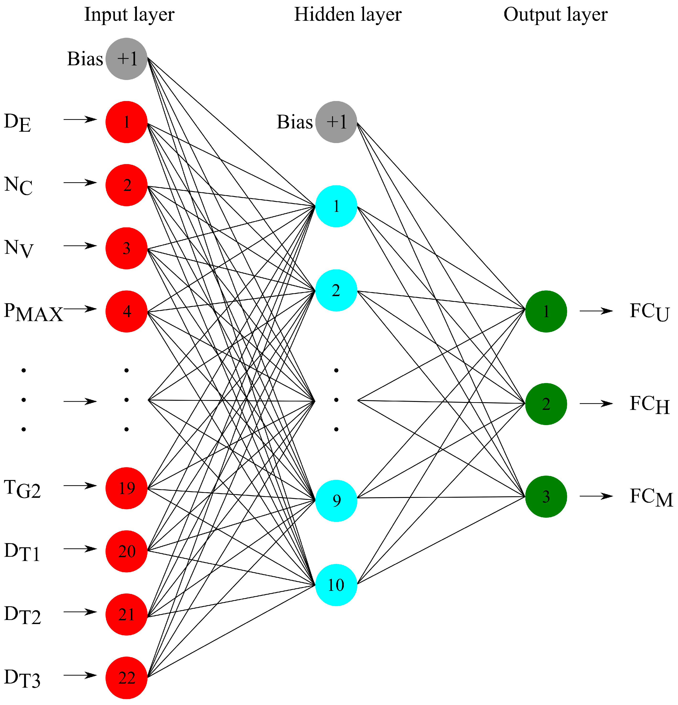
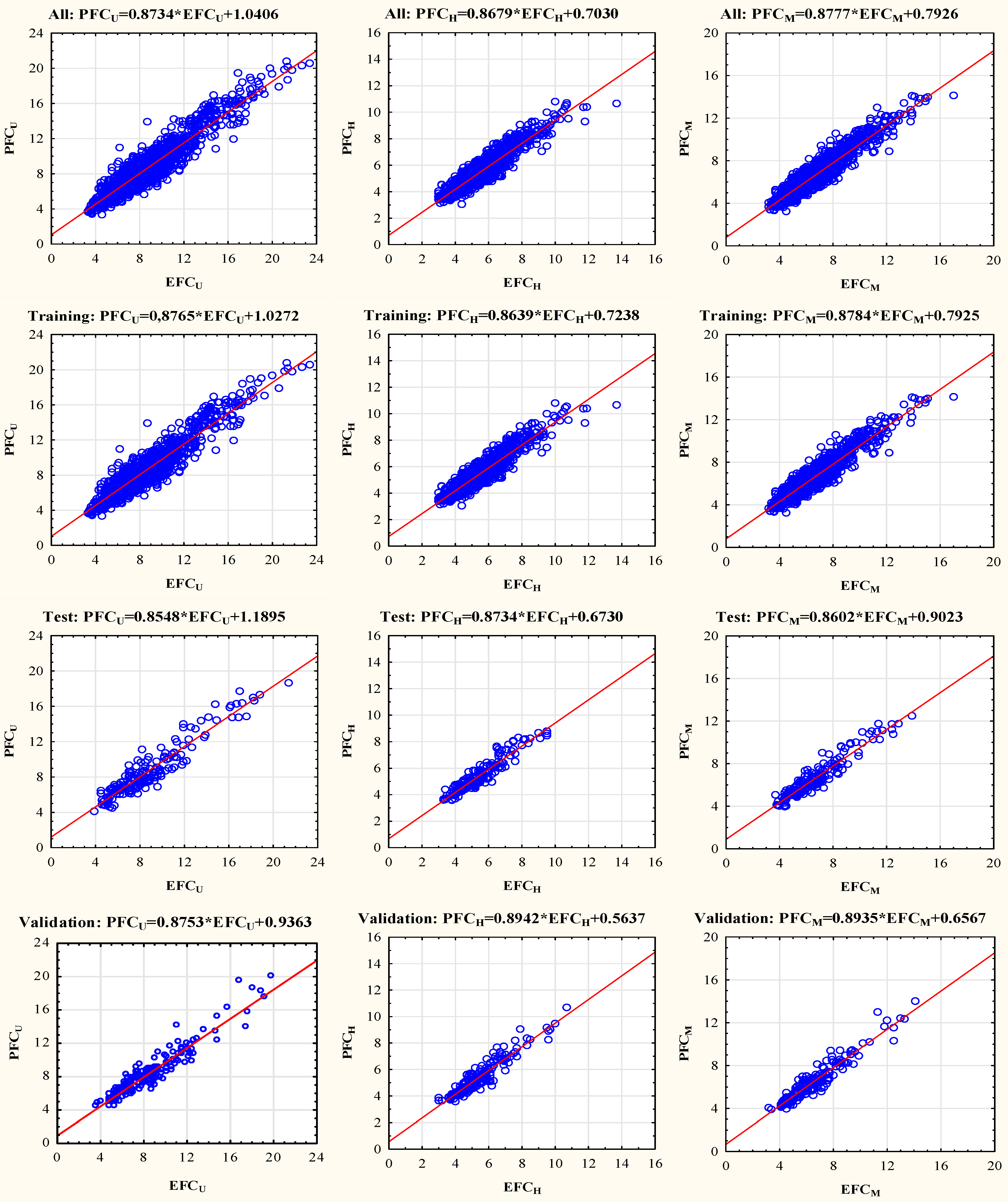
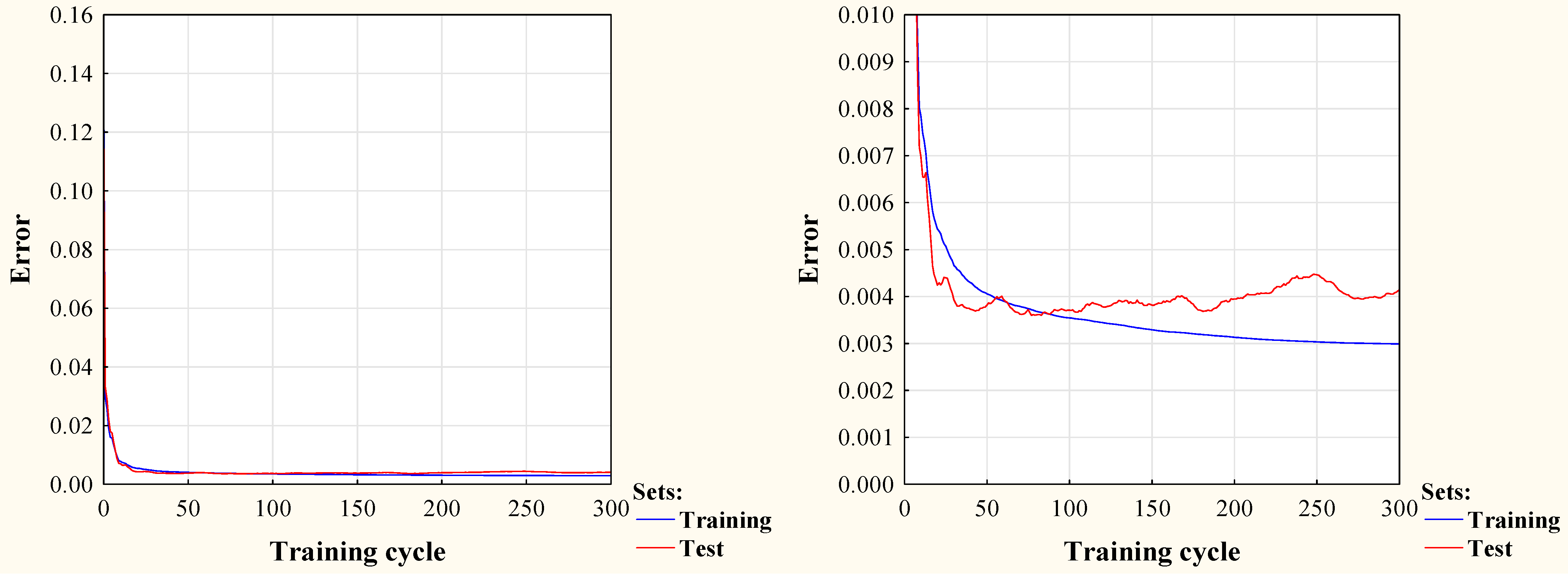
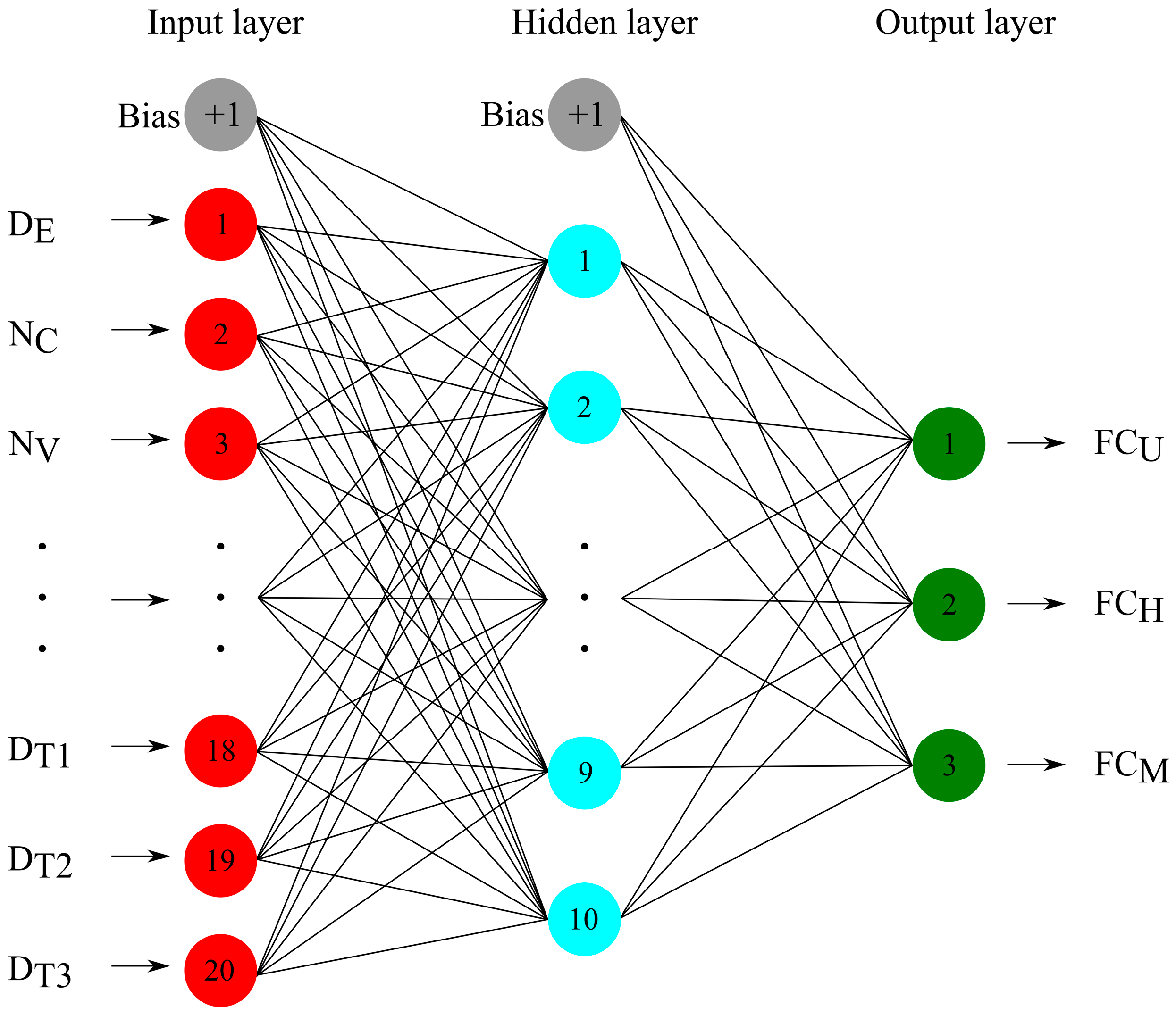
| Research Area | Structure of ANNs | Predicted Variables | Results | Publication |
|---|---|---|---|---|
| Fuel consumption of many vehicles | 5-17-17-1 | Fuel consumption | R: 0.94–0.99 MSE < 0.6 | [8] |
| 3-128-1 3-64-64-1 3-(4 × 32)-1 3-(8 × 16)-1 | Fuel consumption | R2: 0.72–0.78 | [33] | |
| 9-4-1 9-6-1 9-8-1 9-10-1 9-12-1 | Fuel consumption | R = 0.82 | [34] | |
| Diesel engine | 4-8-2 4-14-3 4-13-5 | BSEC (Brake Specific Energy Consumption) BTE (Brake Thermal Efficiency) ID (Ignition Delay) CD (Combustion Duration) CPP (Cylinder Peak Pressure) Exhaust emission (CO, CO2, UBHC, NOx, Smoke) | R2 > 0.98 R: 0.95–1.00 MAPE < 5% | [35] |
| 3-9-5 | Brake thermal efficiency BSEC Exhaust emission (NOx, UBHC, CO) | R2 > 0.99 MAPE < 4% | [36] | |
| 3-7-2 | Fuel consumption Exhaust temperature | MAPE < 3% | [37] | |
| 4-10-10-5 | BSEC BTE Exhaust emission (CO2, NOx) PM (Particulate matter) | R2 > 0.98 MAPE < 5% | [38] | |
| 4-2-7 4-4-7 4-6-7 4-8-7 4-10-7 | BSFC (Brake Specific Fuel Consumption) BTE Exhaust temperature Exhaust emission (CO, HC, NOx) Smoke | R: 0.97–0.99 MSE = 0.06 | [39] | |
| 3-8-9 | Exhaust gas temperature BSFC Power Torque Smoke Exhaust emission (CO, CO2, HC, NOX) | R2: 0.80–0.96 | [40] | |
| Gasoline engine | 4-13-1 4-15-1 | Torque BSFC | R > 0.98 MAPE < 3% | [32] |
| Stirling engine | 4-H-2 (H = {3,4,5,…,13}) | Power Torque | R2 > 0.97 | [41] |
| 3-10-1 | Power | R2 > 0.97 | [42] | |
| HCNG (hydrogen enriched compressed natural gas) engine | 4-H-1 (H = {2,4,6,…,30}) | BSFC Torque Exhaust emission (NOx, CO, THC, CH4) | R: 0.79–1.00 | [43] |
| Electric vehicles | 5-5-1 | Energy consumption | R = 0.81 MAPE < 5% | [44] |
| Type of Variables | Name of Variable | Designation | (Unit)/Nominal Values | |
|---|---|---|---|---|
| Input | Quantitative | Cubic capacity | DE | (cm3) |
| Quantity of cylinders | NC | (unitless) | ||
| Quantity of valves | NV | (unitless) | ||
| Maximum power | PMAX | (kW) | ||
| Maximum torque | TMAX | (Nm) | ||
| Compression rate | CR | (unitless) | ||
| Kerb weight of vehicle | WV | (kg) | ||
| Qualitative | Type of engine | ET | Gasoline (ET1) | |
| Diesel (ET2) | ||||
| Hybrid: gasoline + electric (ET3) | ||||
| Hybrid: diesel + electric (ET4) | ||||
| Fuel injection | FI | Indirect (FI1) | ||
| Direct (FI2) | ||||
| Type of charge | BT | Naturally aspirated (BT1) | ||
| Turbocharger (BT2) | ||||
| Biturbo (BT3) | ||||
| Compressor (BT4) | ||||
| Gearbox | TG | Manual (TG1) | ||
| Automatic (TG2) | ||||
| Drivetrain | DT | FWD (DT1) | ||
| RWD (DT2) | ||||
| AWD (DT3) | ||||
| Output | Quantitative | Fuel consumption in the urban cycle | FCU | (l/100 km) |
| Fuel consumption in the extraurban cycle | FCH | (l/100 km) | ||
| Fuel consumption in the mixed cycle | FCM | (l/100 km) | ||
| Variable | Mean | Median | Min. | Max. | SD |
|---|---|---|---|---|---|
| Cubic capacity DE (cm3) | 2096.00 | 1984 | 799 | 6299 | 831.36 |
| Quantity of cylinders NC | 4.48 | 4 | 2 | 12 | 1.18 |
| Quantity of valves NV | 17.38 | 16 | 6 | 48 | 5.15 |
| Max. power PMAX (kW) | 132.86 | 119.3 | 40.3 | 469.8 | 65.22 |
| Max. torque TMAX (Nm) | 311.77 | 305.0 | 88.0 | 1000.0 | 135.55 |
| Compression rate CR | 13.23 | 11.30 | 8.20 | 19.50 | 3.25 |
| Kerb weight of vehicle WV (kg) | 1463.70 | 1450.0 | 750.0 | 2656.0 | 294.14 |
| Fuel consumption in the urban cycle FCU (l/100 km) | 8.47 | 7.8 | 3.3 | 23.4 | 3.06 |
| Fuel consumption in the extraurban cycle FCH (l/100 km) | 5.37 | 5.1 | 3.0 | 13.7 | 1.35 |
| Fuel consumption in the mixed cycle FCM (l/100 km) | 6.51 | 6.1 | 3.2 | 17.0 | 1.94 |
| Variable | DE | NC | NV | PMAX | TMAX | CR | WV |
|---|---|---|---|---|---|---|---|
| Cubic capacity DE | — | 0.9181 | 0.8865 | 0.9040 | 0.8195 | −0.0404 | 0.7646 |
| Quantity of cylinders NC | 0.9181 | — | 0.9085 | 0.8425 | 0.7625 | −0.0812 | 0.6729 |
| Quantity of valves NV | 0.8865 | 0.9085 | — | 0.8396 | 0.7500 | −0.0953 | 0.6967 |
| Max. power PMAX | 0.9040 | 0.8425 | 0.8396 | — | 0.8367 | −0.2092 | 0.6999 |
| Max. torque TMAX | 0.8195 | 0.7625 | 0.7500 | 0.8367 | — | 0.2390 | 0.7984 |
| Compression rate CR | −0.0404 | −0.0812 | −0.0953 | −0.2092 | 0.2390 | — | 0.1653 |
| Kerb weight of vehicle WV | 0.7646 | 0.6729 | 0.6967 | 0.6999 | 0.7984 | 0.1653 | — |
| No | Network Structure | Accuracy (Train.) | Accuracy (Test) | Accuracy (Val.) | Error (Train.) | Error (Test) | Error (Valid.) | Algorithm | Activation Functions |
|---|---|---|---|---|---|---|---|---|---|
| 1 | MLP 22-10-3 | 0.9355 | 0.9512 | 0.9359 | 0.9105 | 0.8527 | 0.9431 | BFGS 79 | Tanh/Linear |
| 2 | MLP 22-17-3 | 0.9371 | 0.9507 | 0.9382 | 0.8920 | 0.8617 | 0.9370 | BFGS 84 | Tanh/Linear |
| 3 | MLP 22-21-3 | 0.9286 | 0.9503 | 0.9355 | 1.0156 | 0.8687 | 0.9410 | BFGS 47 | Tanh/Linear |
| 4 | MLP 22-22-3 | 0.9317 | 0.9522 | 0.9321 | 0.9705 | 0.8497 | 1.0237 | BFGS 61 | Tanh/Linear |
| 5 | MLP 22-10-3 | 0.9290 | 0.9518 | 0.9335 | 1.0052 | 0.8300 | 0.9921 | BFGS 46 | Sigmoidal/Linear |
| 6 | MLP 22-25-3 | 0.9332 | 0.9508 | 0.9334 | 0.9496 | 0.8198 | 0.9558 | BFGS 47 | Tanh/Sigmoidal |
| 7 | MLP 22-17-3 | 0.9328 | 0.9502 | 0.9330 | 0.9567 | 0.8454 | 0.9895 | BFGS 41 | Tanh/Sigmoidal |
| 8 | MLP 22-10-3 | 0.9370 | 0.9461 | 0.9432 | 0.8895 | 0.9146 | 0.8218 | BFGS 84 | Exponential/Sigmoidal |
| 9 | MLP 22-15-3 | 0.9397 | 0.9481 | 0.9394 | 0.8639 | 0.8772 | 0.8909 | BFGS 79 | Exponential/Exponential |
| 10 | MLP 22-15-3 | 0.9437 | 0.9467 | 0.9410 | 0.8088 | 0.9110 | 0.8869 | BFGS 110 | Exponential/Sigmoidal |
| Correlation Coefficient | Variable | Set | |||
|---|---|---|---|---|---|
| All | Training | Test | Validation | ||
| r | FCU | 0.9381 | 0.9363 | 0.9450 | 0.9440 |
| FCH | 0.9345 | 0.9331 | 0.9434 | 0.9369 | |
| FCM | 0.9432 | 0.9415 | 0.9499 | 0.9486 | |
| R2 | FCU | 0.9861 | 0.9862 | 0.9859 | 0.9879 |
| FCH | 0.9925 | 0.9939 | 0.9922 | 0.9930 | |
| FCM | 0.9910 | 0.9915 | 0.9907 | 0.9922 | |
| Input Variable | ||||||||||||
|---|---|---|---|---|---|---|---|---|---|---|---|---|
| ET | FI | DE | PMAX | WV | BT | TMAX | NC | CR | DT | NV | TG | |
| Wj | 13.5900 | 4.0619 | 3.0441 | 2.7966 | 2.4305 | 1.9532 | 1.5222 | 1.3797 | 1.3096 | 1.2963 | 1.1049 | 1.0000 |
| No | Network Structure | Accuracy (Train.) | Accuracy (Test) | Accuracy (Val.) | Error (Train.) | Error (Test) | Error (Valid.) | Algorithm | Activation Functions |
|---|---|---|---|---|---|---|---|---|---|
| 1 | MLP 20-10-3 | 0.9474 | 0.9519 | 0.9229 | 0.7486 | 0.8446 | 1.0351 | BFGS 413 | Exponential/Sigmoidal |
| 2 | MLP 20-10-3 | 0.9439 | 0.9462 | 0.9343 | 0.8061 | 0.9071 | 0.9479 | BFGS 151 | Exponential/Sigmoidal |
| 3 | MLP 20-10-3 | 0.9335 | 0.9441 | 0.9416 | 0.9389 | 0.9572 | 0.8343 | BFGS 77 | Exponential/Sigmoidal |
| 4 | MLP 20-10-3 | 0.9360 | 0.9438 | 0.9382 | 0.9007 | 0.9896 | 0.9210 | BFGS 99 | Exponential/Sigmoidal |
| 5 | MLP 20-10-3 | 0.9422 | 0.9457 | 0.9196 | 0.8284 | 0.9414 | 1.0715 | BFGS 187 | Exponential/Sigmoidal |
| 6 | MLP 20-10-3 | 0.9425 | 0.9445 | 0.9347 | 0.8157 | 0.9350 | 0.9668 | BFGS 178 | Exponential/Sigmoidal |
| 7 | MLP 20-10-3 | 0.9332 | 0.9450 | 0.9338 | 0.9436 | 0.9386 | 0.9031 | BFGS 74 | Exponential/Sigmoidal |
| 8 | MLP 20-10-3 | 0.9438 | 0.9482 | 0.9243 | 0.8020 | 0.9066 | 1.0611 | BFGS 229 | Exponential/Sigmoidal |
| 9 | MLP 20-10-3 | 0.9445 | 0.9492 | 0.9199 | 0.7908 | 0.8676 | 1.1337 | BFGS 265 | Exponential/Sigmoidal |
| 10 | MLP 20-10-3 | 0.9361 | 0.9459 | 0.9373 | 0.9077 | 0.9304 | 0.8999 | BFGS 93 | Exponential/Sigmoidal |
| Correlation Coefficient | Variable | Set | |||
|---|---|---|---|---|---|
| All | Training | Test | Validation | ||
| r | FCU | 0.9350 | 0.9327 | 0.9430 | 0.9433 |
| FCH | 0.9318 | 0.9300 | 0.9417 | 0.9358 | |
| FCM | 0.9396 | 0.9377 | 0.9477 | 0.9457 | |
| R2 | FCU | 0.9855 | 0.9856 | 0.9851 | 0.9879 |
| FCH | 0.9922 | 0.9937 | 0.9919 | 0.9928 | |
| FCM | 0.9904 | 0.9910 | 0.9901 | 0.9917 | |
| Input Variable | |||||||||||
|---|---|---|---|---|---|---|---|---|---|---|---|
| ET | FI | DE | BT | WV | PMAX | DT | TMAX | NC | CR | NV | |
| Wj | 16.0194 | 3.2997 | 3.2528 | 2.4795 | 2.2873 | 1.8756 | 1.3758 | 1.3124 | 1.2954 | 1.2855 | 1.0993 |
| Neural Network | Variable | Set | Prediction Error | ||
|---|---|---|---|---|---|
| MSE | RMSE | MAPE (%) | |||
| MLP 22-10-3 | FCU | All | 1.1232 | 1.0598 | 10.32 |
| Training | 1.1215 | 1.0590 | 10.36 | ||
| Test | 1.2216 | 1.1053 | 10.88 | ||
| Validation | 1.0387 | 1.0192 | 8.39 | ||
| FCH | All | 0.2307 | 0.4803 | 6.96 | |
| Training | 0.2362 | 0.4860 | 6.41 | ||
| Test | 0.1920 | 0.4382 | 7.05 | ||
| Validation | 0.2249 | 0.4742 | 5.35 | ||
| FCM | All | 0.4166 | 0.6454 | 7.99 | |
| Training | 0.4213 | 0.6491 | 8.01 | ||
| Test | 0.4157 | 0.6447 | 8.07 | ||
| Validation | 0.3799 | 0.6164 | 5.06 | ||
| MLP 20-10-3 | FCU | All | 1.1777 | 1.0852 | 10.57 |
| Training | 1.1824 | 1.0874 | 10.64 | ||
| Test | 1.2799 | 1.1313 | 11.13 | ||
| Validation | 1.0383 | 1.0190 | 9.51 | ||
| FCH | All | 0.2404 | 0.4903 | 7.07 | |
| Training | 0.2471 | 0.4971 | 6.50 | ||
| Test | 0.1978 | 0.4447 | 7.18 | ||
| Validation | 0.2292 | 0.4788 | 6.80 | ||
| FCM | All | 0.4425 | 0.6652 | 8.16 | |
| Training | 0.4484 | 0.6696 | 8.24 | ||
| Test | 0.4368 | 0.6609 | 8.16 | ||
| Validation | 0.4010 | 0.6332 | 7.56 | ||
Publisher’s Note: MDPI stays neutral with regard to jurisdictional claims in published maps and institutional affiliations. |
© 2021 by the authors. Licensee MDPI, Basel, Switzerland. This article is an open access article distributed under the terms and conditions of the Creative Commons Attribution (CC BY) license (https://creativecommons.org/licenses/by/4.0/).
Share and Cite
Ziółkowski, J.; Oszczypała, M.; Małachowski, J.; Szkutnik-Rogoż, J. Use of Artificial Neural Networks to Predict Fuel Consumption on the Basis of Technical Parameters of Vehicles. Energies 2021, 14, 2639. https://doi.org/10.3390/en14092639
Ziółkowski J, Oszczypała M, Małachowski J, Szkutnik-Rogoż J. Use of Artificial Neural Networks to Predict Fuel Consumption on the Basis of Technical Parameters of Vehicles. Energies. 2021; 14(9):2639. https://doi.org/10.3390/en14092639
Chicago/Turabian StyleZiółkowski, Jarosław, Mateusz Oszczypała, Jerzy Małachowski, and Joanna Szkutnik-Rogoż. 2021. "Use of Artificial Neural Networks to Predict Fuel Consumption on the Basis of Technical Parameters of Vehicles" Energies 14, no. 9: 2639. https://doi.org/10.3390/en14092639
APA StyleZiółkowski, J., Oszczypała, M., Małachowski, J., & Szkutnik-Rogoż, J. (2021). Use of Artificial Neural Networks to Predict Fuel Consumption on the Basis of Technical Parameters of Vehicles. Energies, 14(9), 2639. https://doi.org/10.3390/en14092639


