Abstract
State-of-charge (SOC) estimation of lithium-ion batteries (LIBs) is the basis of other state estimations. However, its accuracy can be affected by many factors, such as temperature and ageing. To handle this bottleneck issue, we here propose a joint SOC-SOH estimation method considering the influence of the temperature. It combines the Forgetting Factor Recursive Least Squares (FFRLS) algorithm, Total Least Squares (TLS) algorithm, and Unscented Kalman Filter (UKF) algorithm. First, the FFRLS algorithm is used to identify and update the parameters of the equivalent circuit model in real time under different battery ageing degrees. Then, the TLS algorithm is used to estimate the battery SOH to improve the prior estimation accuracy of SOC. Next, the SOC is calculated by the UKF algorithm, and finally, a more accurate SOH can be obtained according to the UKF-based SOC trajectory. The battery-in-the-loop experiments are utilized to verify the proposed algorithm. For the cases of temperature change up to 35 °C and capacity decay up to 10%, our joint estimator can achieve ultra-low errors, bounded by 2%, respectively, for SOH and SOC. The proposed method paves the way for the advancement of battery use in applications, such as electric vehicles and microgrid applications.
1. Introduction
Energy crises and environmental pollution are the main obstacles restricting the sustainable development of the economy and society. In this context, electric vehicles (EVs) have developed rapidly worldwide because of their advantages in environmental protection and energy conservation [1,2,3,4,5]. As the core component of EVs, lithium-ion batteries (LIBs) have significant benefits, such as long cycle life, high energy density, and low self-discharge rate [6,7,8,9,10,11]. Since Li-ion batteries are easily affected by usage conditions and environments, a battery management system (BMS) is essential in ensuring battery safety and reliability. State estimation of LIBs is one of the core functions of BMS. Common states include state-of-charge (SOC), state-of-health (SOH), state-of-energy (SOE), state-of-power (SOP), etc. [12,13,14]. SOC and SOH are, respectively, the indicators for remaining driving distance and ageing degree [15,16,17]. However, due to the unaffordable cost of integrating sensors into the batteries [18], these implicit states cannot be directly measured by commercial BMSs. As a response, state estimation techniques, which indirectly calculate the internal states of the batteries from available signals such as current, voltage, and temperature, are gaining popularity.
SOC represents the ratio of the remaining capacity of LIB to its full charge capacity, whose estimation is the basis of the other state observers. However, as revealed by [19], the accuracy of the SoC calculator is affected by factors such as battery ageing, ambient temperature, and sensor noise. Therefore, conventional approaches, such as the ampere-hour integral method and standard OCV method, are less effective in this kind of complicated usage scenario. Compared with these simple algorithms, model-based approaches exhibit better adaptiveness to these factors and have become the mainstream for online SOC estimation [20]. Commonly used models can be categorized into three types, namely, first-principle models, electric circuit models, and data-driven models.
First-principle models refer to models that describe the process of chemical changes in batteries. Pseudo Two-Dimensional (P2D) model and Single Particle (SP) model [21,22,23,24] are the most representative examples. Though theoretically accurate, they require a deep understanding of electrochemical natures, which may vary with battery materials [17,25]. In addition, these models are usually complicated to implement due to the involvement of partial differential equations [26]. Therefore, they are more suitable for theoretical analysis and less effective for onboard applications.
Data-driven models, as the name implies, rely purely on the data. Commonly seen examples include neural networks (NN) [27], support vector regression (SVR) [28], Gaussian process regression (GPR) [29], and extreme learning machine (ELM) [30,31]. Without using any prior knowledge of the chemistry nature, data-driven models can be used to describe all types of LIBs. However, as a common issue for these data-driven methods, these models require a large amount of data for training to improve accuracy, and their generalization to untrained cases is usually weak. Since the real-life battery using profiles contain high uncertainties, considerable training data should be used to ensure estimation accuracy in different scenarios.
Compared with the above two model types, ECM, which uses RC networks to simulate battery dynamics, offers a good balance between complexity and accuracy. As a result, various methods are combined with the ECMs to implement SOC estimation. Commonly used algorithms include Kalman Filters [32,33,34], Particle Filters [35], and some light-weighted approaches such as Luenberger observer [36], PI observer [37], sliding mode observer [38], and local least squares [39].
It is worth pointing out that the accuracy of these algorithms relies on not only the quality of the filtering methods but also the modeling accuracy. As is the case with most electrochemical systems, the model parameters of LIBs will change gradually with battery ageing and temperature, and the resulted model mismatch will lead to large SOC estimation errors [40]. Understanding that the SOH estimation also relies on an accurate SOC estimation, joint state estimation frameworks for SOC and SOH have been developed to handle this kind of circular dependence. Specifically, Yu et al. [40] used the Recursive Least Square (RLS) algorithm to realize the online parameter identification of ECM and then combined it with the adaptive H∞ filter to estimate battery SOH. Tan et al. [41] proposed an EKF-RLS-based dynamic parameter identification algorithm with a multi-timescale and conducted an online SOH estimation based on the SVR algorithm. Yan et al. [42] estimated the battery SOH and predicted the remaining service life based on Lebesgue sampling. Tang et al. [43] used V-min EKF to estimate the SOC and explored a balancing current ratio technique to estimate the SOH for all cells in a battery pack.
Though effective, it is worth pointing out that most joint SOC-SOH estimation frameworks do not consider the influence of temperature on model parameters. In addition, they do not use an estimated state (e.g., SOH) to improve the accuracy of the other estimates (e.g., SOC), leaving space to improve the overall accuracy. Aiming at these issues, we here propose a joint SOC-SOH estimation method. Specifically, the FFRLS algorithm is first used to identify the parameters of ECM in the battery ageing process online, and the battery model is then updated in real-time. Next, the battery capacity and SOH are calculated by using the TLS algorithm with the identified parameters. Based on the updated model parameters and capacity, the SOC is estimated using the UKF algorithm. Finally, the battery SOH is calculated again using the TLS algorithm and the estimated SOC trajectories. The effectiveness of our “two-stage” estimation strategy is verified with the battery-in-the-loop experiments. The main potential contributions of this work can be summarized as follows: (1) A new joint SOC-SOH estimation framework is proposed. In particular, a “two-stage” estimation strategy is proposed to improve SOH estimation accuracy. (2) SOC and SOH are accurately co-estimated online with a low computational cost against temperature change and battery ageing.
2. Battery Modeling
2.1. Equivalent Circuit Model
ECM balances model accuracy and complexity and is widely used in battery state estimation [44,45]. The RC elements in the ECM can simulate the chemical diffusion and polarization process inside the battery, and it is divided into 1RC, 2RC, 3RC, and n-RC models. In this study, the 1RC model is used because it provides a good balance between model robustness and complexity [46]. Its structure is shown in Figure 1.
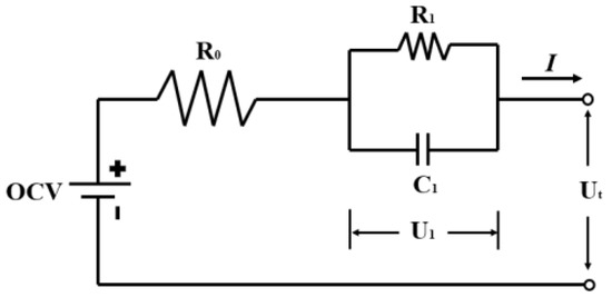
Figure 1.
1RC model.
The mathematical expression of the 1RC model is as follows:
where subscript k is the time k, Ut is the battery terminal voltage, U1 is the polarization voltage, I is the working current (positive when charging the battery), R0 is ohmic resistance, R1 is polarization resistance, C1 is polarization capacitance, τ1 is time constant, t is the time, OCV() is a nonlinear function describing the relationship between the battery’s OCV and SOC, and SOC is the battery’s state-of-charge, also defined as the remaining percentage of the battery’s available capacity.
Recall the transfer function of the RC series circuit in the frequency domain:
where s is a complex variable in the Laplace transform.
By using bilinear transformation to discretize Equation (4), we get:
where ΔT is the sampling interval, z is a complex variable in the Z-transformation.
According to the 1RC equivalent circuit structure, the converted transfer function is:
Substituting Equation (5) into Equation (6) yields the transfer function as:
Equation (7) can be further simplified as follows:
which can be given as follows:
Or equivalently:
By converting Equation (8) back to the (discretized) time domain and assuming that the battery’s OCV tends to be stable in a short period (say, OCVk approximately equals to OCVk−1), we have:
Equation (15) can be re-written as:
with and .
It is worth pointing out that our modeling strategy is different from those in Ref [47], as OCV is also treated as a parameter to be identified in Equation (16). In this way, we can use the identified OCV to implement the calculation of battery SOH while avoiding the “circular dependence” issue (see Section 3.1 for details).
2.2. Online Parameter Identification
To ensure the modeling accuracy under various battery temperatures and ageing degrees, we need to update the model parameters in real time. At present, model identification algorithms, such as the PSO and GA, are widely adopted [48]. However, these algorithms suffer from high computational costs and are, therefore, not suitable for online applications. The least square method is simple and requires no prior statistics. It is widely used for online parameter identification [49]. However, a converged least square algorithm is less sensitive to the new data [50], resulting in a gradual increase in error. To address this issue, we here introduce the FFRLS algorithm to identify the model parameters online. The process of online identification by the FFRLS algorithm is shown in Figure 2. The specific process is as follows:
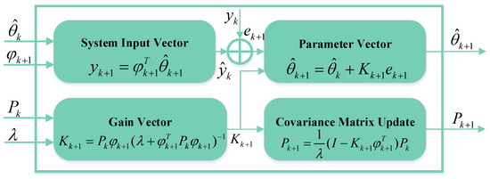
Figure 2.
The parameter identification process of the FFRLS algorithm.
- (1)
- System input vector:
- (2)
- Estimated error:
- (3)
- Gain vector:
- (4)
- Parameter vector to be evaluated:
- (5)
- Update covariance matrix:where is the estimated parameter vector in Equation (17), e is estimation error, K is the gain matrix, P is the covariance matrix, I is the identity matrix, and λ is the forgetting factor, which is added to the conventional RLS algorithm to reduce the weight of old data and improve the accuracy of online parameter identification under dynamic conditions.
When using the FFRLS algorithm, initial parameters (a1, a2 and a3) are calculated by interpolating the data obtained from the parameter identification of fresh battery. Then, the vector θk is determined, and the measurement vector and input vector yk are determined according to the measured current and voltage data. Afterwards, the estimated error ek is calculated. The gain vector Kk is calculated based on the covariance matrix Pk, measurement vector , and forgetting factor λ. Finally, the estimated parameter vector θk is calculated, and the model parameters can then be updated according to Equations (9)–(14). It should be noted that the measured battery voltage and current change with the battery ageing and temperature. In this case, the model parameters identified in real-time by the FFRLS algorithm will change to minimize the model and measured voltages. Therefore, the proposed algorithm can realize the real-time online identification and update of battery model parameters and OCV under complex conditions.
3. Joint SOC-SOH Estimation Method
3.1. SOH Estimation
The battery’s SOH is not only an important indicator of the ageing status but also a key prior knowledge for accurate SOC estimation. We do have multiple algorithms to obtain battery SOH, such as using ICA-based calculous [51]. However, when an accurate SOC trajectory is available, the most used battery capacity estimation method is the “Two-Point” [52]. This method calculates the battery’s current capacity based on the change in charge and SOC between the time interval t1->t2, which can be described as follows:
where and are the corresponding battery SOC at two different times, t1 and t2, respectively, Cap0 is the battery’s initial capacity, and η is Coulomb efficiency, which is commonly treated as 1.
In this work, our SOH estimation contains two stages. In the first stage, a SOH value is calculated following the idea of Equation (22), where the SOC is obtained by feeding the OCV identified from Equations (17)–(21) into a static OCV-SOC lookup table. Though less accurate, this SOH can be used to compensate for the large capacity deviation of the aged batteries to facilitate the follow-up SOC calculation. In the second stage, the SOH is calculated again following the idea of Equation (22), but the SOC is obtained from the powerful UKF algorithm (see Section 3.2 for details) to improve its accuracy. Noting that two different models are utilized to obtain the SOC, our two-stage SOH estimator will not suffer from the issue of “circular dependence”. In this work, our OCV-SOC trajectory is obtained through the Hybrid Pulse Power Characteristic (HPPC) test at 25 °C, a detailed experimental procedure that can be found in our previous work [53]. For clarity, the identified OCV-SOC curve of our battery is shown in Figure 3.
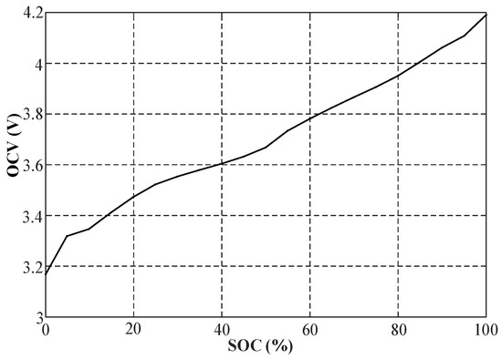
Figure 3.
OCV-SOC curve.
Noting that the “Two-Point” method suffers from the local perturbance in SOC estimation, rather than directly using Equation (22), the total least square (TLS) algorithm [54] is used to estimate the capacity online. Re-write Equation (22) as:
Marking , and , the following expression can be obtained:
where β1 is an estimated constant, β2 is an estimated coefficient with Cap = 1/β2 and vi is the noise in the estimation process.
By accumulating data from time m to time n (1 < m < n), Equation (24) can be expressed in vector form as:
Then, Equation (25) can be converted into matrix form:
where Y is the observation vector, X is a known matrix, is the parameter vector, and V is the random error vector.
The parameter vector H can be solved by the analytic expression of the TLS algorithm:
where σn+1 is the smallest singular value of [X Y], E is the identity matrix. Then, the TLS-based capacity can be estimated by:
Dividing the estimated capacity by the fresh-cell-capacity, we obtain the estimated SOH:
The above process is utilized for both the first-stage and the second-stage SOH estimation. The only difference here is the method of acquiring battery SOC.
3.2. SOC Estimation
3.2.1. UKF Algorithm
Kalman Filter (KF) algorithm is widely used as the state observer, and the EKF algorithm, which uses Tayer expansion to provide first-order model linearization, is the most commonly used for SOC estimation in BMS [55]. However, batteries are highly nonlinear systems, and using only first-order approximation will significantly influence the estimation accuracy. Therefore, the UKF algorithm [56,57] is employed to estimate SOC in this study. UKF algorithm deals with nonlinear systems by using the idea of the probability distribution, which approximately replaces the linearization of the propagation mode of statistical characteristics in EKF with an unscented transform (UT). UT will not directly omit the higher-order terms but obtain some sampling points near the estimation points according to certain calculation rules and use these sampling points to approximate the probability density function of the state [58]. In general, UT could achieve 3-order approximating accuracy for Gaussian inputs and at least 2-order accuracy for non-Gaussian cases. The specific implementation process is as follows:
- (1)
- Obtaining the 2n + 1 Sigma points:where Z is the sampling point after UT, is the mean value of random variables, n is the dimension of the state vector, and P is the error covariance matrix.
- (2)
- Weighting of each Sigma point:where is the adjustment parameter, α denotes the distance from the sampling point to the mean point, which is usually set to a small positive number, is usually taken as 0 or 3, and β describes the distribution information.
After UT, the statistical characteristics of the new sampling points are used to describe the nonlinear equation, which avoids the error caused by directly ignoring the high-order terms and effectively improves the filter accuracy.
3.2.2. SOC Estimation Based on UKF Algorithm
To implement the UKF algorithm, we first discrete the battery model, with the results given in Equations (32)–(34). Here is the sampling interval, R0 is ohmic resistance, R1 is polarization resistance, τ1 is time constant, Ik is working current, η is Coulomb efficiency, CapTLS is the current capacity estimated online by the TLS algorithm, wk is state transition noise, and vk is measurement noise.
Then, the current is treated as the system’s input, and SOC and polarization voltage are regarded as state variables and estimated simultaneously from the measured voltage. The state vectors SOC and U1,k can also be written in the form of vectors, which is shown in Equation (35). The system observation value yk is the battery’s terminal voltage Ut,k, as shown in Equation (36), and the working current Ik is treated as the system excitation, as shown in Equation (37).
With these definitions, Equations (35) and (37) can be re-written as
with , , and .
The state equation and observation equation of a nonlinear system can be expressed in Equations (39) and (40):
According to UT, state transition equation, and observation equation, the calculation process of the UKF algorithm is listed in Algorithm 1.
| Algorithm 1. The calculation process of the UKF algorithm. |
| (1) Initialization parameters:The error covariance matrix P, usually taken as . |
| (2) Iterative calculation, k = 1,2,…,N: (a) The state vector is transformed by the UT, and the Sigma points of the state vector xk and the weight of each Sigma point are calculated according to Equations (30) and (31). (b) State transfer of Sigma points: (e) The new Sigma points are brought into the observation Equation (40), and the observation values are obtained: (g) Calculating the Kalman gain Kk: |
The online SOC estimation can be completed by substituting Equations (39) and (40) into the above iterative process. The parameters updated online in the FFRLS algorithm will improve the accuracy of the UKF algorithm, including state vector xk and error covariance Pk. The joint SOC-SOH estimation process of LIBs based on the FFRLS-TLS-UKF algorithm is shown in Figure 4.
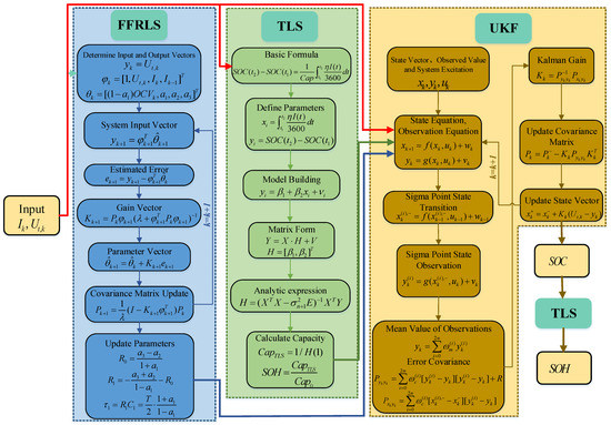
Figure 4.
Flow chart of joint SOC-SOH estimation.
4. Experimental Validation
4.1. Experimental Setup
The schematic of the experimental setup is shown in Figure 5. The experimental device is composed of a high-precision battery test system (CT-4008-5V12A-DB), an upper computer, a temperature chamber (BTH-150C), and the 18650 cylindrical battery. The battery test system is connected to the battery in the incubator to control the charging/discharging current and collect data. The upper computer can input commands to control other experimental equipment and store data. The temperature chamber is used to observe and adjust the test temperature. The performance parameters of the experimental battery are shown in Table 1.
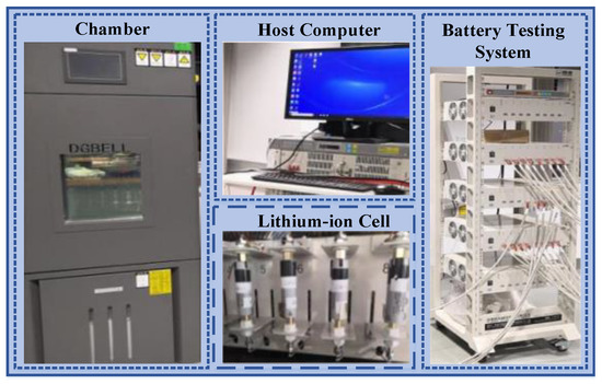
Figure 5.
Experimental setup.

Table 1.
Battery performance parameters.
4.2. Experimental Results
In this paper, the ageing experiments are designed to verify the feasibility of the joint SOC-SOH estimation method based on the FFRLS-TLS-UKF algorithm. The steps of the ageing experiment are shown in Figure 6. The temperature chamber was adjusted to 45 °C, 25 °C, and 10 °C, respectively. Then, the battery was charged at a constant current to SOC = 100% and SOC = 80% at each temperature. Third, the battery was discharged with a constant current of 1/2C to SOC = 0% and SOC = 30%. Fourth, the above process was repeated twice at each temperature and the temperature was adjusted to 25 °C for the basic performance test after completing the cycle, including the standard capacity test, the HPPC test, and the New European Driving Cycle (NEDC) test. The above process is defined as an ageing cycle. The frequency of data acquisition in this paper is 1Hz. The current in an NEDC test is shown in Figure 7.
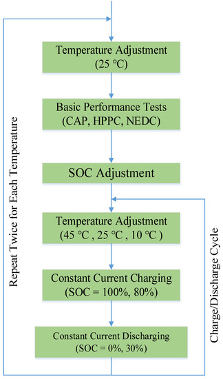
Figure 6.
Steps of Ageing Experiment.
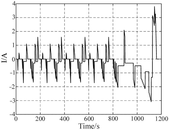
Figure 7.
Current in NEDC.
4.2.1. Results of Parameter Identification
In this study, we first use the PSO algorithm to identify the parameters of the fresh battery at 25 °C to obtain an initial value. The whole SOC region is divided into 10 subregions. In each subregion, the PSO algorithm is used to identify the model parameters offline. Therefore, 10 groups of model parameters are obtained. FFRLS algorithm is then utilized to acquire the model parameters of the target battery online. The results of parameter identification after the first ageing cycle are shown in Figure 8. We can see that the model accuracy is very high (RMSEs of four parameters are 15 mV, 8 mΩ, 16 mΩ and 15 ms, respectively), and the identification value is consistent with the reference value. In addition, the model error in the low SOC region (SOC < 20%) is slightly larger, which is the deficiency of the integer order ECMs.
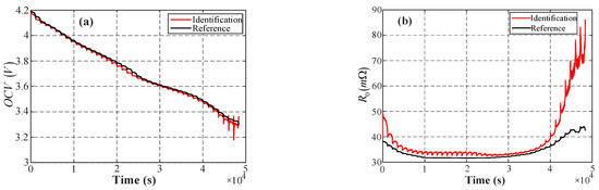
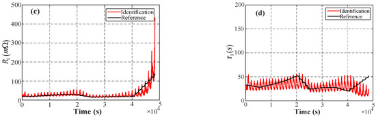
Figure 8.
Results of parameter identification after the first ageing cycle: (a) OCV, (b) R0, (c) R1, and (d) τ1.
To better illustrate the effectiveness of the proposed identification, we compare the error between the model’s and the measured battery terminal voltage over the full SOC range. Here, six groups of NEDC test data of LIBs with different ageing degrees (SOH down to 86.9%) are selected. The error of terminal voltage between real-time updating and non-updating parameters is shown in Figure 9, with RMSE given in Table 2.
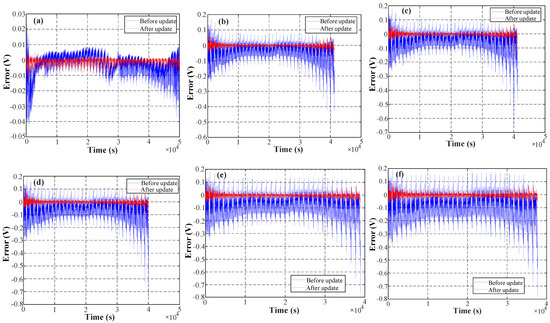
Figure 9.
Terminal voltage error under different ageing degrees: (a) SOH = 96.2%, (b) SOH = 90.2%, (c) SOH = 89.8%, (d) SOH = 89.2%, (e) SOH = 88.3%, and (f) SOH = 86.9%.
Table 2.
Model errors of batteries with different ageing degrees.
The blue lines in Figure 9 denote the modeling error of using the fresh battery’s parameter, and the red line marks the error corresponding to the parameter-adaptive models. As shown in Figure 9, the error of terminal voltage after parameter updating is significantly reduced by 81%, implying an improved modeling accuracy.
Table 2 lists the RMSE of terminal voltage in the whole SOC range before and after parameter updating. When model mismatch does not exist, the parameter-fixed RC model could also achieve a relatively low error (approximately 10 mV). However, this error increases with ageing, especially when SOH < 90%. After using FFRLS to update the model parameters, RMSE drops to 20 mV, which is satisfactory for general engineering use.
4.2.2. Results of SOC Estimation
To verify the effectiveness of the proposed FFRLS-TLS-UKF algorithm in SOC estimation, we use six groups of NEDC test data with different ageing degrees (SOH = 96.2%, 90.2%, 89.8%, 89.2%, 88.3%, and 86.9%) for online parameter identification. The TLS algorithm is used to estimate SOH (in the first stage) to improve the accuracy of prior estimation in the UKF algorithm. Then, SOC is estimated by the UKF algorithm. SOC estimation results under different ageing degrees are shown in Figure 10. The mean absolute error (MAE) and RMSE of SOC estimation are shown in Table 3. The blue line in Figure 10 denotes the SOC reference value obtained by the accurate current integration in our lab, which can be regarded as the referenced value; the green line denotes the SOC estimation results based on the FFRLS-TLS-UKF algorithm; and the red line denotes the SOC estimation results obtained by the UKF algorithm without considering parameter updating. To test the convergence speed of the proposed algorithm, we manually added an initial error of 5% in SOC estimation, and the current and voltage errors are set to ±0.001A/V.
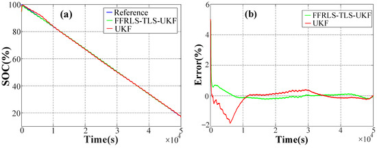
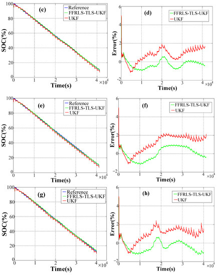
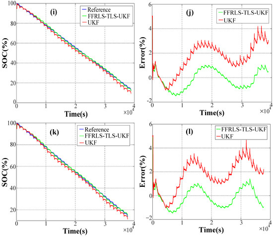
Figure 10.
Results and errors of SOC estimation under different ageing degrees: (a,b) SOH = 96.2%; (c,d) SOH = 90.2%; (e,f) SOH = 89.8%; (g,h) SOH = 89.2%; (i,j) SOH = 88.3%; (k,l) SOH = 86.9%.
Table 3.
MAE and RMSE of SOC estimation.
It can be clearly seen that the SOC estimation using the FFRLS-TLS-UKF algorithm can converge quickly to 2% with the help of real-time updating of model parameters and SOH, even if the capacity difference between the modeling and target batteries exceeds 10% (ranges from 100% to 86.9%). On the contrary, the SOC estimation error without considering parameter updating gradually increases to 4%. It can be concluded that the proposed joint estimation scheme can greatly improve SOC estimation accuracy during battery ageing by at least 50%.
4.2.3. Results of SOH Estimation
After the online model parameter identification, the first-stage SOH (denoted as SOH1 in the following discussions) is estimated by the TLS algorithm. Then, SOH1 is used in SOC estimation to improve accuracy. After SOC estimation, the second-stage SOH (denoted as SOH2 in the following discussions) can be obtained by feeding the estimated SOC trajectories into the TLS algorithm. For comparison, a benchmarking algorithm that calculates the SOH from the UKF-based SOC trajectory (without parameter update) is also tested, whose result is denoted as SOH3. The SOH estimation results during the battery ageing process and their errors are shown in Figure 11, with RMSE listed in Table 4.
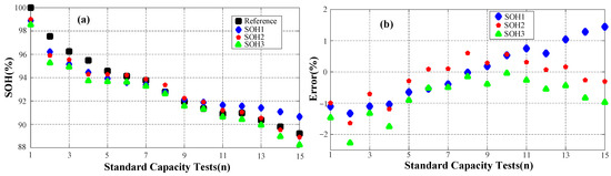
Figure 11.
SOH estimation: (a) Results, and (b) Errors.
Table 4.
RMSE of SOH estimation.
By comparing SOH2 and SOH3, it is straightforward to see that the SOC accuracy could directly influence the performance of the “Two-Point” SOH estimator. The SOC obtained from the conventional UKF approach suffers from a large chattering issue for aged batteries, and the resulted SOH error becomes large, exceeding 2%. When comparing SOH1 and SOH2, we can see that the second-stage SOH updating is effective. This result agrees with the fact that the FFRLS-UKF algorithm with TLS-updated SOH can provide better SOC estimation accuracy than feeding the online identified OCV into the OCV-SOC lookup table. When comparing SOH1 and SOH3, it is interesting to note that using a powerful UKF algorithm to handle parameter-fixed models is less effective than using a simple FFRLS algorithm to update the parameter-fixed model. This result highlights the importance of adaptive parameter updating in the field of battery management. In addition, the first-stage estimator (SOH1) can also be used independently as an efficient, lightweight SOH observer to save computation.
5. Conclusions
An accurate SOC estimation is key to reducing range anxiety, but it is commonly influenced by the inevitable battery ageing, noting that the battery parameters change gradually with degradation. Here, a joint SOC-SOH estimation method for LIBs based on the FFRLS-TLS-UKF algorithm is proposed to tackle this bottleneck issue, and the following conclusions are drawn:
(1) The FFRLS algorithm is proposed to identify the parameters online. The experimental results indicate that the error of terminal voltage decreases after parameter updating, bounded by 20 mV, even if >10% model mismatch in battery ageing exists;
(2) A two-stage SOH estimator based on the TLS algorithm is proposed, and its error is lower than 2%, exhibiting first-class accuracy. The first-stage SOH estimator can also be used independently to reduce algorithm complexity;
(3) The FFRLS-TLS-UKF algorithm proposed in this paper can effectively improve the accuracy of SOC estimation. The SOC accuracy estimated by the proposed algorithm is almost twice that estimated by the traditional EKF algorithm. The error is kept within 2% even if there are initial SOC errors, modeling mismatches, and measurement noises.
Author Contributions
Conceptualization, M.Y. and X.L.; methodology, M.Y.; software, M.Y.; validation, M.Y. and X.L.; formal analysis, M.Y.; investigation, M.Y. and J.W.; resources, M.Y. and Y.Y.; data curation, M.Y. and Y.Z.; writing–original draft preparation, M.Y., and X.T.; writing–review and editing, X.T. and X.L.; visualization, M.Y. and W.M.; supervision, X.L., F.G. and Y.Z. All authors have read and agreed to the published version of the manuscript.
Funding
This research was funded by the National Natural Science Foundation of China (Grant Nos. 51977131 and 52277223), Natural Science Foundation of Shanghai (19ZR1435800), State Key Laboratory of Automotive Safety and Energy (KF2020), Shanghai Science and Technology Development Fund (19QA1406200) and the Hong Kong RGC Postdoctoral Fellowship Scheme (PDFS2122-6S06).
Conflicts of Interest
The corresponding author is an editor of this special issue. The manuscript is being handled independently by the other editors.
References
- Wang, X.; Wei, X.; Zhu, J.; Dai, H.; Zheng, Y.; Xu, X.; Chen, Q. A review of modeling, acquisition, and application of lithium-ion battery impedance for onboard battery management. eTransportation 2020, 7, 100093. [Google Scholar] [CrossRef]
- Song, Z.; Yang, X.-G.; Yang, N.; Delgado, F.P.; Hofmann, H.; Sun, J. A study of cell-to-cell variation of capacity in parallel-connected lithium-ion battery cells. eTransportation 2021, 7, 100091. [Google Scholar] [CrossRef]
- Hao, X.; Yuan, Y.B.; Wang, H.W.; Ouyang, M.G. Plug-in hybrid electric vehicle utility factor in China cities: Influencing factors, empirical research, and energy and environmental application. eTransportation 2021, 10, 100138. [Google Scholar] [CrossRef]
- Hu, G.; Huang, P.; Bai, Z.; Wang, Q.; Qi, K. Comprehensively analysis the failure evolution and safety evaluation of automotive lithium ion battery. eTransportation 2021, 10, 100140. [Google Scholar] [CrossRef]
- Su, L.; Wu, M.; Li, Z.; Zhang, J. Cycle life prediction of lithium-ion batteries based on data-driven methods. eTransportation 2021, 10, 100137. [Google Scholar] [CrossRef]
- Zheng, Y.; Lu, Y.; Gao, W.; Han, X.; Feng, X.; Ouyang, M. Micro-Short-Circuit Cell Fault Identification Method for Lithium-Ion Battery Packs Based on Mutual Information. IEEE Trans. Ind. Electron. 2021, 68, 4373–4381. [Google Scholar] [CrossRef]
- Lai, X.; Chen, Q.; Tang, X.; Zhou, Y.; Gao, F.; Guo, Y.; Bhagat, R.; Zheng, Y. Critical review of life cycle assessment of lithium-ion batteries for electric vehicles: A lifespan perspective. eTransportation 2022, 12, 100169. [Google Scholar] [CrossRef]
- Chen, Q.; Lai, X.; Gu, H.; Tang, X.; Gao, F.; Han, X.; Zheng, Y. Investigating carbon footprint and carbon reduction potential using a cradle-to-cradle LCA approach on lithium-ion batteries for electric vehicles in China. J. Clean. Prod. 2022, 369, 133342. [Google Scholar] [CrossRef]
- Sun, P.; Zhang, H.; Jiang, F.-C.; He, Z.-Z. Self-driven liquid metal cooling connector for direct current high power charging to electric vehicle. eTransportation 2021, 10, 100132. [Google Scholar] [CrossRef]
- Liu, J.; Wang, Z.; Hou, Y.; Qu, C.; Hong, J.; Lin, N. Data-driven energy management and velocity prediction for four-wheel-independent-driving electric vehicles. eTransportation 2021, 9, 100119. [Google Scholar] [CrossRef]
- Wildfeuer, L.; Lienkamp, M. Quantifiability of inherent cell-to-cell variations of commercial lithium-ion batteries. eTransportation 2021, 9, 100129. [Google Scholar] [CrossRef]
- Tang, X.; Liu, K.; Wang, X.; Gao, F.; Macro, J.; Widanage, W.D. Model Migration Neural Network for Predicting Battery Aging Trajectories. IEEE Trans. Transp. Electrif. 2020, 6, 363–374. [Google Scholar] [CrossRef]
- Tang, X.; Wang, Y.; Chen, Z. A method for state-of-charge estimation of LiFePO4 batteries based on a dual-circuit state observer. J. Power Sources 2015, 296, 23–29. [Google Scholar] [CrossRef]
- Lai, X.; He, L.; Wang, S.; Zhou, L.; Zhang, Y.; Sun, T.; Zheng, Y. Co-estimation of state of charge and state of power for lithium-ion batteries based on fractional variable-order model. J. Clean. Prod. 2020, 255, 120203. [Google Scholar] [CrossRef]
- Hu, X.; Feng, F.; Liu, K.; Zhang, L.; Xie, J.; Liu, B. State estimation for advanced battery management: Key challenges and future trends. Renew. Sustain. Energy Rev. 2019, 114, 109334. [Google Scholar] [CrossRef]
- Lai, X.; Huang, Y.; Gu, H.; Han, X.; Feng, X.; Dai, H.; Zheng, Y.; Ouyang, M. Remaining discharge energy estimation for lithium-ion batteries based on future load prediction considering temperature and ageing effects. Energy 2021, 238, 121754. [Google Scholar] [CrossRef]
- Qin, P.; Sun, J.; Yang, X.; Wang, Q. Battery thermal management system based on the forced-air convection: A review. eTransportation 2021, 7, 100097. [Google Scholar] [CrossRef]
- Zhu, S.; Han, J.; An, H.-Y.; Pan, T.-S.; Wei, Y.-M.; Song, W.-L.; Chen, H.-S.; Fang, D. A novel embedded method for in-situ measuring internal multi-point temperatures of lithium ion batteries. J. Power Sources 2020, 456, 227981. [Google Scholar] [CrossRef]
- Xiong, R.; Yu, Q.; Wang, L.Y.; Lin, C. A novel method to obtain the open circuit voltage for the state of charge of lithium ion batteries in electric vehicles by using H infinity filter. Appl. Energy 2017, 207, 346–353. [Google Scholar] [CrossRef]
- Xiong, R.; Cao, J.; Yu, Q.; He, H.; Sun, F. Critical Review on the Battery State of Charge Estimation Methods for Electric Vehicles. IEEE Access 2018, 6, 1832–1843. [Google Scholar] [CrossRef]
- Han, X.; Ouyang, M.; Lu, L.; Li, J.; Zheng, Y.; Li, Z. A comparative study of commercial lithium ion battery cycle life in electrical vehicle: Aging mechanism identification. J. Power Sources 2014, 251, 38–54. [Google Scholar] [CrossRef]
- Yin, H.; Ma, S.; Li, H.; Wen, G.; Santhanagopalan, S.; Zhang, C. Modeling strategy for progressive failure prediction in lithium-ion batteries under mechanical abuse. eTransportation 2021, 7, 100098. [Google Scholar] [CrossRef]
- Deshpande, R.D.; Bernardi, D.M. Modeling Solid-Electrolyte Interphase (SEI) Fracture: Coupled Mechanical/Chemical Degradation of the Lithium Ion Battery. J. Electrochem. Soc. 2017, 164, A461–A474. [Google Scholar] [CrossRef]
- Wu, B.; Lu, W. Mechanical Modeling of Particles with Active Core–Shell Structures for Lithium-Ion Battery Electrodes. J. Phys. Chem. C 2017, 121, 19022–19030. [Google Scholar] [CrossRef]
- Ali, Y.; Lee, S. An integrated experimental and modeling study of the effect of solid electrolyte interphase formation and Cu dissolution on CuCo2O4-based Li-ion batteries. Int. J. Energy Res. 2022, 46, 3017–3033. [Google Scholar] [CrossRef]
- Laue, V.; Röder, F.; Krewer, U. Practical identifiability of electrochemical P2D models for lithium-ion batteries. J. Appl. Electrochem. 2021, 51, 1253–1265. [Google Scholar] [CrossRef]
- Cui, Z.; Wang, L.; Li, Q.; Wang, K. A comprehensive review on the state of charge estimation for lithium-ion battery based on neural network. Int. J. Energy Res. 2022, 46, 5423–5440. [Google Scholar] [CrossRef]
- Shu, X.; Li, G.; Shen, J.; Lei, Z.; Chen, Z.; Liu, Y. A uniform estimation framework for state of health of lithium-ion batteries considering feature extraction and parameters optimization. Energy 2020, 204, 117957. [Google Scholar] [CrossRef]
- Che, Y.; Deng, Z.; Tang, X.; Lin, X.; Nie, X.; Hu, X. Lifetime and Aging Degradation Prognostics for Lithium-ion Battery Packs Based on a Cell to Pack Method. Chin. J. Mech. Eng. 2022, 35, 4. [Google Scholar] [CrossRef]
- Li, S.; He, H.; Li, J. Big data driven lithium-ion battery modeling method based on SDAE-ELM algorithm and data pre-processing technology. Appl. Energy 2019, 242, 1259–1273. [Google Scholar] [CrossRef]
- Shu, X.; Shen, S.; Shen, J.; Zhang, Y.; Li, G.; Chen, Z.; Liu, Y. State of health prediction of lithium-ion batteries based on machine learning: Advances and perspectives. iScience 2021, 24, 103265. [Google Scholar] [CrossRef] [PubMed]
- Lai, X.; Qiao, D.; Zheng, Y.; Zhou, L. A Fuzzy State-of-Charge Estimation Algorithm Combining Ampere-Hour and an Extended Kalman Filter for Li-Ion Batteries Based on Multi-Model Global Identification. Appl. Sci. 2018, 8, 2028. [Google Scholar] [CrossRef]
- Ling, L.; Sun, D.; Yu, X.; Huang, R. State of charge estimation of Lithium-ion batteries based on the probabilistic fusion of two kinds of cubature Kalman filters. J. Energy Storage 2021, 43, 103070. [Google Scholar] [CrossRef]
- Lai, X.; Yi, W.; Cui, Y.; Qin, C.; Han, X.; Sun, T.; Zhou, L.; Zheng, Y. Capacity estimation of lithium-ion cells by combining model-based and data-driven methods based on a sequential extended Kalman filter. Energy 2020, 216, 119233. [Google Scholar] [CrossRef]
- Tang, X.; Wang, Y.; Zou, C.; Yao, K.; Xia, Y.; Gao, F. A novel framework for Lithium-ion battery modeling considering uncertainties of temperature and aging. Energy Convers. Manag. 2018, 180, 162–170. [Google Scholar] [CrossRef]
- Boulmrharj, S.; Ouladsine, R.; NaitMalek, Y.; Bakhouya, M.; Zine-Dine, K.; Khaidar, M.; Siniti, M. Online battery state-of-charge estimation methods in micro-grid systems. J. Energy Storage 2020, 30, 101518. [Google Scholar] [CrossRef]
- Yang, X.; Chen, Y.; Li, B.; Luo, D. Battery states online estimation based on exponential decay particle swarm optimization and proportional-integral observer with a hybrid battery model. Energy 2020, 191, 116509. [Google Scholar] [CrossRef]
- Zheng, W.; Xia, B.; Wang, W.; Lai, Y.; Wang, M.; Wang, H. State of Charge Estimation for Power Lithium-Ion Battery Using a Fuzzy Logic Sliding Mode Observer. Energies 2019, 12, 2491. [Google Scholar] [CrossRef]
- Zhang, J.; Wang, P.; Gong, Q.; Cheng, Z. SOH estimation of lithium-ion batteries based on least squares support vector machine error compensation model. J. Power Electron. 2021, 21, 1712–1723. [Google Scholar] [CrossRef]
- Yu, Q.; Xiong, R.; Yang, R.; Pecht, M.G. Online capacity estimation for lithium-ion batteries through joint estimation method. Appl. Energy 2019, 255, 113817. [Google Scholar] [CrossRef]
- Tan, X.; Zhan, D.; Lyu, P.; Rao, J.; Fan, Y. Online state-of-health estimation of lithium-ion battery based on dynamic parameter identification at multi timescale and support vector regression. J. Power Sources 2021, 484, 229233. [Google Scholar] [CrossRef]
- Yan, W.; Zhang, B.; Zhao, G.; Tang, S.; Niu, G.; Wang, X. A Battery Management System With a Lebesgue-Sampling-Based Extended Kalman Filter. IEEE Trans. Ind. Electron. 2019, 66, 3227–3236. [Google Scholar] [CrossRef]
- Tang, X.; Gao, F.; Liu, K.; Liu, Q.; Foley, A.M. A Balancing Current Ratio Based State-of-Health Estimation Solution for Lithium-Ion Battery Pack. IEEE Trans. Ind. Electron. 2022, 69, 8055–8065. [Google Scholar] [CrossRef]
- Hu, X.; Li, S.; Peng, H. A comparative study of equivalent circuit models for Li-ion batteries. J. Power Sources 2012, 198, 359–367. [Google Scholar] [CrossRef]
- Lai, X.; Qin, C.; Gao, W.; Zheng, Y.; Yi, W. A State of Charge Estimator Based Extended Kalman Filter Using an Electrochemistry-Based Equivalent Circuit Model for Lithium-Ion Batteries. Appl. Sci. 2018, 8, 1592. [Google Scholar] [CrossRef]
- Lai, X.; Zheng, Y.; Sun, T. A comparative study of different equivalent circuit models for estimating state-of-charge of lithium-ion batteries. Electrochim. Acta 2018, 259, 566–577. [Google Scholar] [CrossRef]
- Wei, Z.; Zou, C.; Leng, F.; Soong, B.H.; Tseng, K.-J. Online Model Identification and State-of-Charge Estimate for Lithium-Ion Battery With a Recursive Total Least Squares-Based Observer. IEEE Trans. Ind. Electron. 2017, 65, 1336–1346. [Google Scholar] [CrossRef]
- Lai, X.; Gao, W.; Zheng, Y.; Ouyang, M.; Li, J.; Han, X.; Zhou, L. A comparative study of global optimization methods for parameter identification of different equivalent circuit models for Li-ion batteries. Electrochim. Acta 2018, 295, 1057–1066. [Google Scholar] [CrossRef]
- Sun, X.; Ji, J.; Ren, B.; Xie, C.; Yan, D. Adaptive Forgetting Factor Recursive Least Square Algorithm for Online Identification of Equivalent Circuit Model Parameters of a Lithium-Ion Battery. Energies 2019, 12, 2242. [Google Scholar] [CrossRef]
- Sun, C.; Lin, H.; Cai, H.; Gao, M.; Zhu, C.; He, Z. Improved parameter identification and state-of-charge estimation for lithium-ion battery with fixed memory recursive least squares and sigma-point Kalman filter. Electrochim. Acta 2021, 387, 138501. [Google Scholar] [CrossRef]
- Tang, X.; Zou, C.; Yao, K.; Chen, G.; Liu, B.; He, Z.; Gao, F. A fast estimation algorithm for lithium-ion battery state of health. J. Power Sources 2018, 396, 453–458. [Google Scholar] [CrossRef]
- Zheng, Y.; Cui, Y.; Han, X.; Dai, H.; Ouyang, M. Lithium-ion battery capacity estimation based on open circuit voltage identification using the iteratively reweighted least squares at different aging levels. J. Energy Storage 2021, 44, 103487. [Google Scholar] [CrossRef]
- Tang, X.; Liu, K.; Liu, Q.; Peng, Q.; Gao, F. Comprehensive study and improvement of experimental methods for obtaining referenced battery state-of-power. J. Power Sources 2021, 512, 230462. [Google Scholar] [CrossRef]
- Markovsky, I.; Van Huffel, S. Overview of total least-squares methods. Signal Process. 2007, 87, 2283–2302. [Google Scholar] [CrossRef]
- Yu, Q.; Wan, C.; Li, J.; E, L.; Zhang, X.; Huang, Y.; Liu, T. An Open Circuit Voltage Model Fusion Method for State of Charge Estimation of Lithium-Ion Batteries. Energies 2021, 14, 1797. [Google Scholar] [CrossRef]
- Lai, X.; Yi, W.; Zheng, Y.; Zhou, L. An All-Region State-of-Charge Estimator Based on Global Particle Swarm Optimization and Improved Extended Kalman Filter for Lithium-Ion Batteries. Electronics 2018, 7, 321. [Google Scholar] [CrossRef]
- Lin, X.; Tang, Y.; Ren, J.; Wei, Y. State of charge estimation with the adaptive unscented Kalman filter based on an accurate equivalent circuit model. J. Energy Storage 2021, 41, 102840. [Google Scholar] [CrossRef]
- He, Z.; Li, Y.; Sun, Y.; Zhao, S.; Lin, C.; Pan, C.; Wang, L. State-of-charge estimation of lithium ion batteries based on adaptive iterative extended Kalman filter. J. Energy Storage 2021, 39, 102593. [Google Scholar] [CrossRef]


Publisher’s Note: MDPI stays neutral with regard to jurisdictional claims in published maps and institutional affiliations. |
© 2022 by the authors. Licensee MDPI, Basel, Switzerland. This article is an open access article distributed under the terms and conditions of the Creative Commons Attribution (CC BY) license (https://creativecommons.org/licenses/by/4.0/).