
Analysis of the Upper Bound of Dynamic Error Obtained during Temperature Measurements


Abstract
1. Introduction
2. General Assumptions
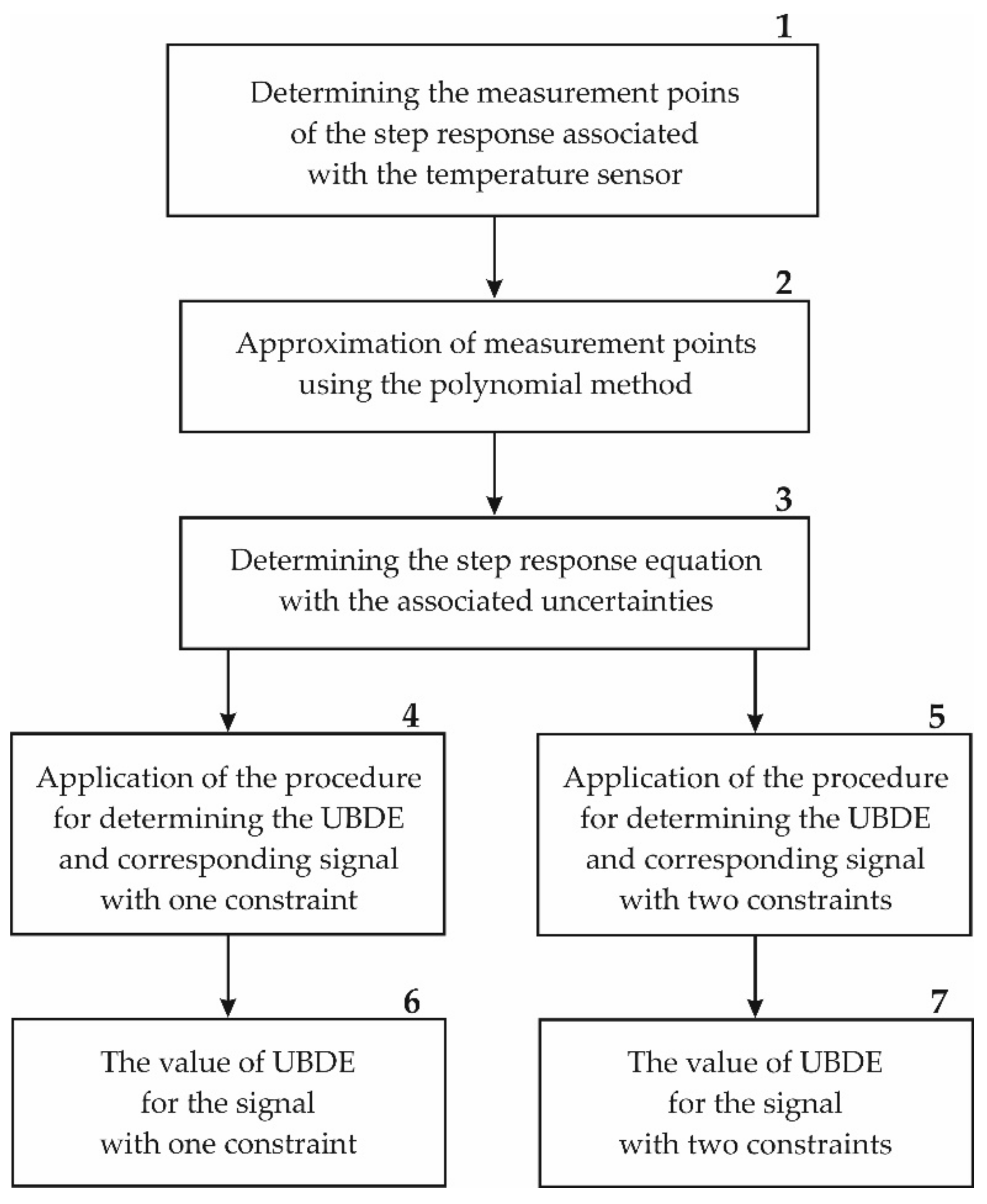
3. Methods and Materials
- 1.
- Determine the pulse function , the duration of which is equal to where is the rate of change constraint. This pulse function can be obtained using the following formula:
- 2.
- Calculate the function based on the function and the impulse response given by Equation (17). The function has the form of the following convolution integral:
- 3.
- Determine the rectangular function as follows:
- 4.
- Determine the function as follows:
- 5.
- Determine the function as follows:
- 6.
- Determine the signal by substituting the function into the function in Equation (16). The signal is the one that produces .
4. Example of the Analysis
5. Conclusions
Author Contributions
Funding
Institutional Review Board Statement
Informed Consent Statement
Data Availability Statement
Conflicts of Interest
Nomenclature
| UBDE | upper bound of dynamic error |
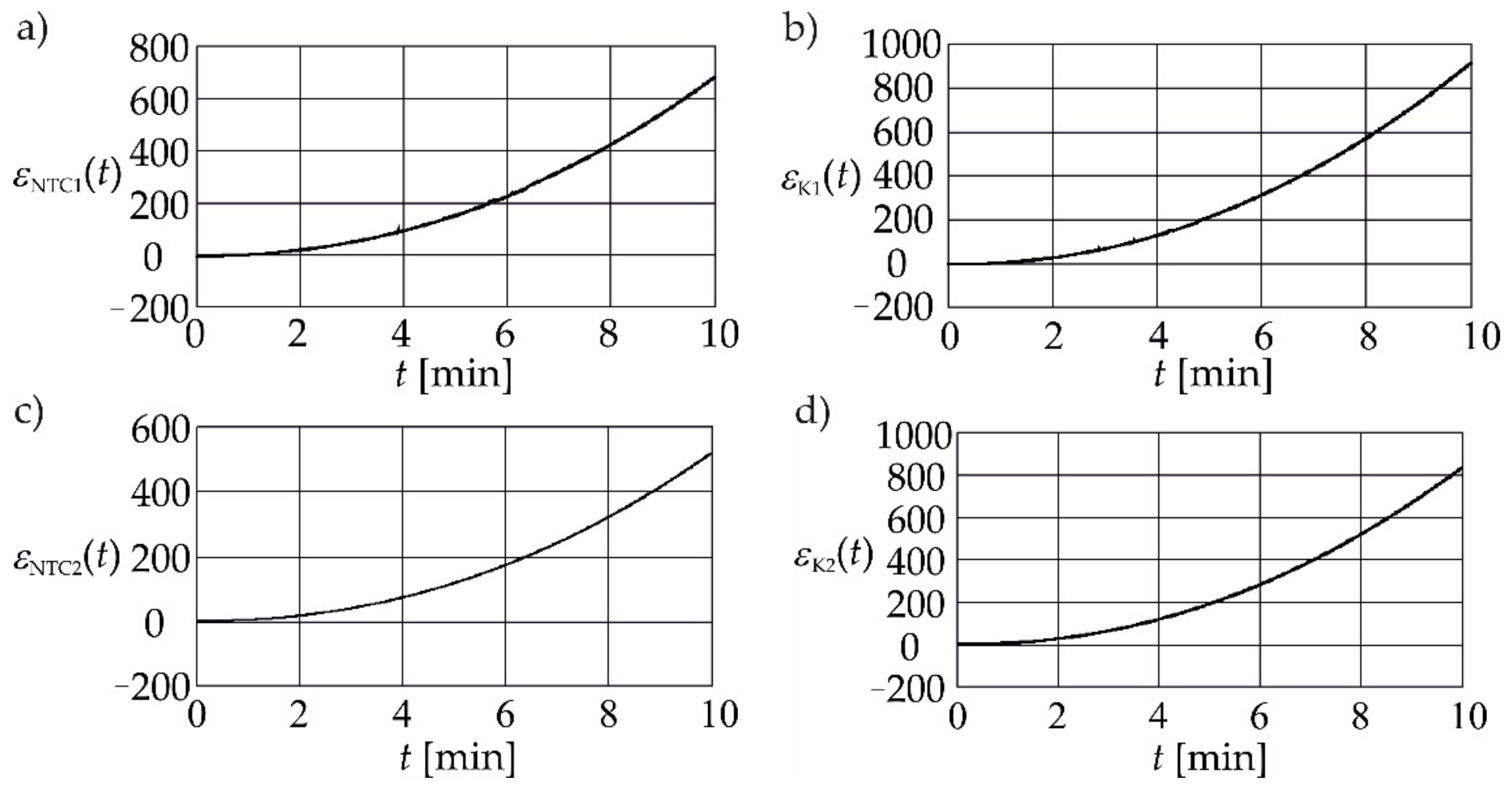
| upper bound of dynamic error produced by a signal with one constraint | |
| upper bound of dynamic error produced by a signal with two constraints | |
| signal with one constraint | |
| signal with two constraints | |
| step response | |
| impulse response | |
| sensor impulse response | |
| reference impulse response | |
| sensor step response | |
| reference step response | |
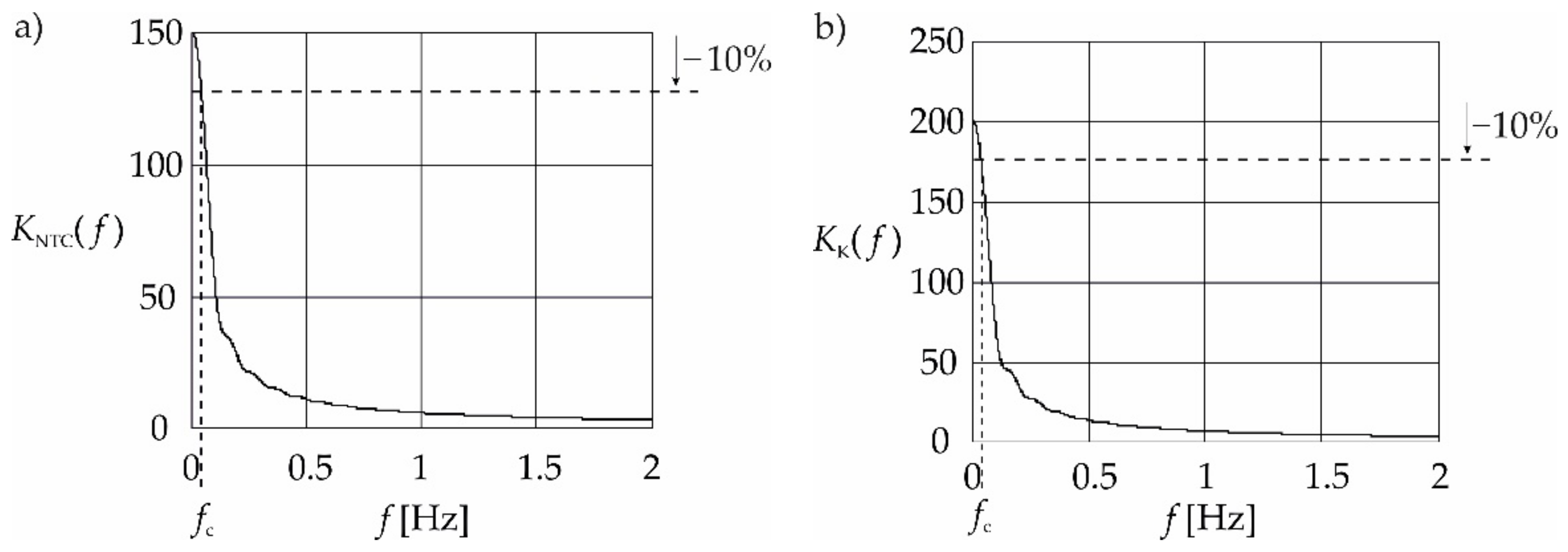
| filter cut-off frequency | |
| number of measurement points | |
| NTC | negative temperature coefficient |
| DAQ | data acquisition |
| Laplace operator | |
| imaginary number | |
| magnitude constraint | |
| rate of change constraint | |
| time of sensor testing | |
| signum function | |
| inverse Laplace transformation | |
| Fourier transformation | |
| error | |
| uncertainty | |
| standard deviation |
References
- Iora, P.; Tribioli, L. Effect of Ambient Temperature on Electric Vehicles’ Energy Consumption and Range: Model Definition and Sensitivity Analysis Based on Nissan Leaf Data. World Electr. Veh. J. 2019, 10, 2. [Google Scholar] [CrossRef]
- Chen, W.H.; Wu, P.H.; Wang, X.D.; Lin, Y.L. Power Output and Efficiency of a Thermoelectric Generator Under Temperature Control. Energy Convers. Manag. 2016, 127, 404–415. [Google Scholar] [CrossRef]
- Cong, Y.; Wall, P.; Li, Q.; Li, Y.; Terzija, V. On the Use of Real-Time Transformer Temperature Estimation for Improving Transformer Operational Tripping Schemes. Int. J. Electr. Power Energy Syst. 2022, 143, 108420. [Google Scholar] [CrossRef]
- Yang, Q.; Liu, G.; Bao, Y.; Chen, Q. Fault Detection of Wind Turbine Generator Bearing Using Attention-Based Neural Networks and Voting-Based Strategy. IEEE/ASME Transact. Mechatron. 2021, in press. [Google Scholar] [CrossRef]
- Coulibaly, A.; Zioui, N.; Bentouba, S.; Kelouwani, S.; Bourouis, M. Use of Thermoelectric Generators to Harvest Energy from Motor Vehicle Brake Discs. Case Stud. Therm. Eng. 2021, 28, 101379. [Google Scholar] [CrossRef]
- Masser, R.; Hoffmann, K.H. Optimal Control for a Hydraulic Recuperation System Using Endoreversible Thermodynamics. Appl. Sci. 2021, 11, 5001. [Google Scholar] [CrossRef]
- Pałka, R.; Woronowicz, K. Linear Induction Motors in Transportation Systems. Energies 2021, 14, 2549. [Google Scholar] [CrossRef]
- Głowacz, A.; Tadeusiewicz, R.; Legutko, S.; Caesarendra, W.; Irfan, M.; Liu, H.; Brumercik, F.; Gutten, M.; Sułowicz, M.; Daviu, J.A.A.; et al. Fault Diagnosis of Angle Grinders and Electric Impact Drills Using Acoustic Signals. Appl. Acoust. 2021, 179, 108070. [Google Scholar] [CrossRef]
- Koritsoglou, K.; Christou, V.; Ntritsos, G.; Tsoumanis, G.; Tsipouras, M.G.; Giannakeas, N.; Tzallas, A.T. Improving the Accuracy of Low-Cost Sensor Measurements for Freezer Automation. Sensors 2020, 20, 6389. [Google Scholar] [CrossRef]
- Shiratsu, A.; Coury, H.J.C.G. Reliability and Accuracy of Different Sensors of a Flexible Electrogoniometer. Clin. Biomech. 2003, 18, 682–684. [Google Scholar] [CrossRef]
- Septiana, R.; Roihan, I.; Koestoer, R.A. Testing a Calibration Method for Temperature Sensors in Different Working Fluids. J. Adv. Res. Fluid Mech. Therm. Sci. 2020, 68, 84–93. [Google Scholar] [CrossRef]
- BIPM; IEC; IFCC; ILAC; ISO; IUPAP; OIML. Guide to the Expression of Uncertainty in Measurement. Supplement 2-Extension to any Number of Output Quantities; International Organization for Standardization: Geneva, Switzerland, 2011. [Google Scholar]
- Morris, A.S. Measurement and Instrumentation Principles; Butterworth-Heinemann Linacre House: Oxford, UK, 2001; ISBN 0-7506-5081-8. [Google Scholar]
- Kim, K.; Kim, J.; Jiang, X.; Kim, T. Static Force Measurement Using Piezoelectric Sensors. J. Sens. 2021, 2021, 6664200. [Google Scholar] [CrossRef]
- Chen, C.M.; Chang, H.L.; Lee, C.Y. The Dynamic Properties at Elevated Temperature of the Thermoplastic Polystyrene Matrix Modified with Nano-Alumina Powder and Thermoplastic Elastomer. Polymers 2022, 14, 3319. [Google Scholar] [CrossRef] [PubMed]
- Augustin, S.; Fröhlich, T.; Ament, C. Dynamic Properties of Contact Thermometers for High Temperatures. Measurement 2014, 51, 387–392. [Google Scholar] [CrossRef]
- Zhong, K.; Zheng, F.; Wu, H.; Qin, C.; Xu, X. Dynamic Changes in Temperature Extremes and their Association with Atmospheric Circulation Patterns in the Songhua River Basin, China. Appl. Acoust. 2017, 190, 77–88. [Google Scholar] [CrossRef]
- Tomczyk, K.; Ostrowska, K. Procedure for the extended calibration of temperature sensors. Measurements 2022, 196, 111239. [Google Scholar] [CrossRef]
- Tomczyk, K. Monte Carlo-based Procedure for Determining the Maximum Energy at the Output of Accelerometers. Energies 2020, 13, 1552. [Google Scholar] [CrossRef]
- Layer, E.; Tomczyk, K. Measurements, Modelling and Simulation of Dynamic Systems; Springer: Berlin/Heidelberg, Germany, 2010; ISBN 978-3-642-04588-2. [Google Scholar]
- Dichev, D.; Koev, H.; Bakalova, T.; Louda, P.A. A Model of the Dynamic Error as a Measurement Result of Instruments Defining the Parameters of Moving Objects. Meas. Sci. Rev. 2014, 14, 183–189. [Google Scholar] [CrossRef]
- Tomczyk, K. Special signals in the calibration of systems for measuring dynamic quantities. Measurement 2014, 49, 148–152. [Google Scholar] [CrossRef]
- Tomczyk, K. Application of Genetic Algorithm to Measurement System Calibration Intended for Dynamic Measurement. Metrol. Meas. Syst. 2006, XIII, 93–103. [Google Scholar]
- Elia, M.; Taricco, G.; Viterbo, E. Optimal Energy Transfer in Band-Limited Communication Channels. IEEE Trans. Inf. Theory 1999, 45, 2020–2029. [Google Scholar] [CrossRef][Green Version]
- Kabashkin, I.; Kundler, J. Reliability of Sensor Nodes in Wireless Sensor Networks of Cyber Physical Systems. Procedia Comput. Sci. 2017, 104, 380–384. [Google Scholar] [CrossRef]
- Layer, E.; Tomczyk, K. Determination of Non-Standard Input Signal Maximizing the Absolute Error. Metrol. Meas. Syst. 2009, 17, 199–208. [Google Scholar]
- Dudzik, M.; Tomczyk, K.; Jagiełło, S.A. Analysis of the Error Generated by the Voltage Output Accelerometer Using the Optimal Structure of an Artificial Neural Network. In Proceedings of the 19th International Conference on Research and Education in Mechatronics (REM), Delft, The Netherlands, 7–8 June 2018; pp. 7–11. [Google Scholar] [CrossRef]
- Rutland, N.K. The Principle of Matching: Practical Conditions for Systems with Inputs Restricted in Magnitude and Rate of Change. IEEE Trans. Autom. Control 1994, 39, 550–553. [Google Scholar] [CrossRef]
- Santos, A.; Liu, N.; Jrad, M. AUSTRET: An Automated Step Response Testing Tool for Building Automation and Control Systems. Energies 2021, 14, 3972. [Google Scholar] [CrossRef]
- Liu, T.; Gao, F. Step response identification of stable processes. In Industrial Process Identification and Control Design; Liu, T., Gao, F., Eds.; Springer: Berlin/Heidelberg, Germany, 2012; pp. 13–84. [Google Scholar] [CrossRef]
- Isermann, R.; Münchhof, M. Identification of Dynamic Systems; Springer: Berlin/Heidelberg, Germany, 2010; ISBN 978-3-540-78878-2. [Google Scholar]
- Kollar, I. On Frequency-Domain Identification of Linear Systems. IEEE Trans. Instrum. Meas. 1993, 42, 2–6. [Google Scholar] [CrossRef]
- Schubert, M.; Münch, C.; Schuurman, S.; Poulain, V.; Kita, J.; Moos, R. Novel Method for NTC Thermistor Production by Aerosol Co-Deposition and Combined Sintering. Sensors 2019, 19, 1632. [Google Scholar] [CrossRef]
- Manjhi, K.S.; Kumar, R. Performance Assessment of K-type, E-type and J-type Coaxial Thermocouples on the Solar Light Beam for Short Duration Transient Measurements. Measurement 2019, 146, 343–355. [Google Scholar] [CrossRef]
- Guijarro, L.; Vidal, J.R.; Pla, V.; Naldi, M. Economic Analysis of a Multi-Sided Platform for Sensor-Based Services in the Internet of Things. Sensors 2019, 19, 373. [Google Scholar] [CrossRef]
- Politi, B.; Foucaran, A.; Camara, N. Low-Cost Sensors for Indoor PV Energy Harvesting Estimation Based on Machine Learning. Energies 2022, 15, 1144. [Google Scholar] [CrossRef]
- Subair, S.; Abraham, L. Analysis of Different Temperature Sensors for Space Applications. Int. J. Innov. Sci. Eng. Technol. 2014, 1, 35–40. [Google Scholar]
- Chen, C.-H.; Hong, C.-M.; Lin, W.-M.; Wu, Y.-C. Implementation of an Environmental Monitoring System Based on IoTs. Electronics 2022, 11, 1596. [Google Scholar] [CrossRef]
- Study of Temperature Transducers. Available online: https://www.scientechworld.com/pdf/study-of-temperature-transducers.pdf. (accessed on 20 August 2022).
- Sun, B.; Liu, H.; Zhou, S.; Li, W. Evaluating the Performance of Polynomial Regression Method with Different Parameters during Color Characterization. Math. Probl. Eng. 2014, 2014, 418651. [Google Scholar] [CrossRef]
- Ostertagova, E. Modelling Using Polynomial Regression. Procedia Eng. 2021, 48, 500–506. [Google Scholar] [CrossRef]


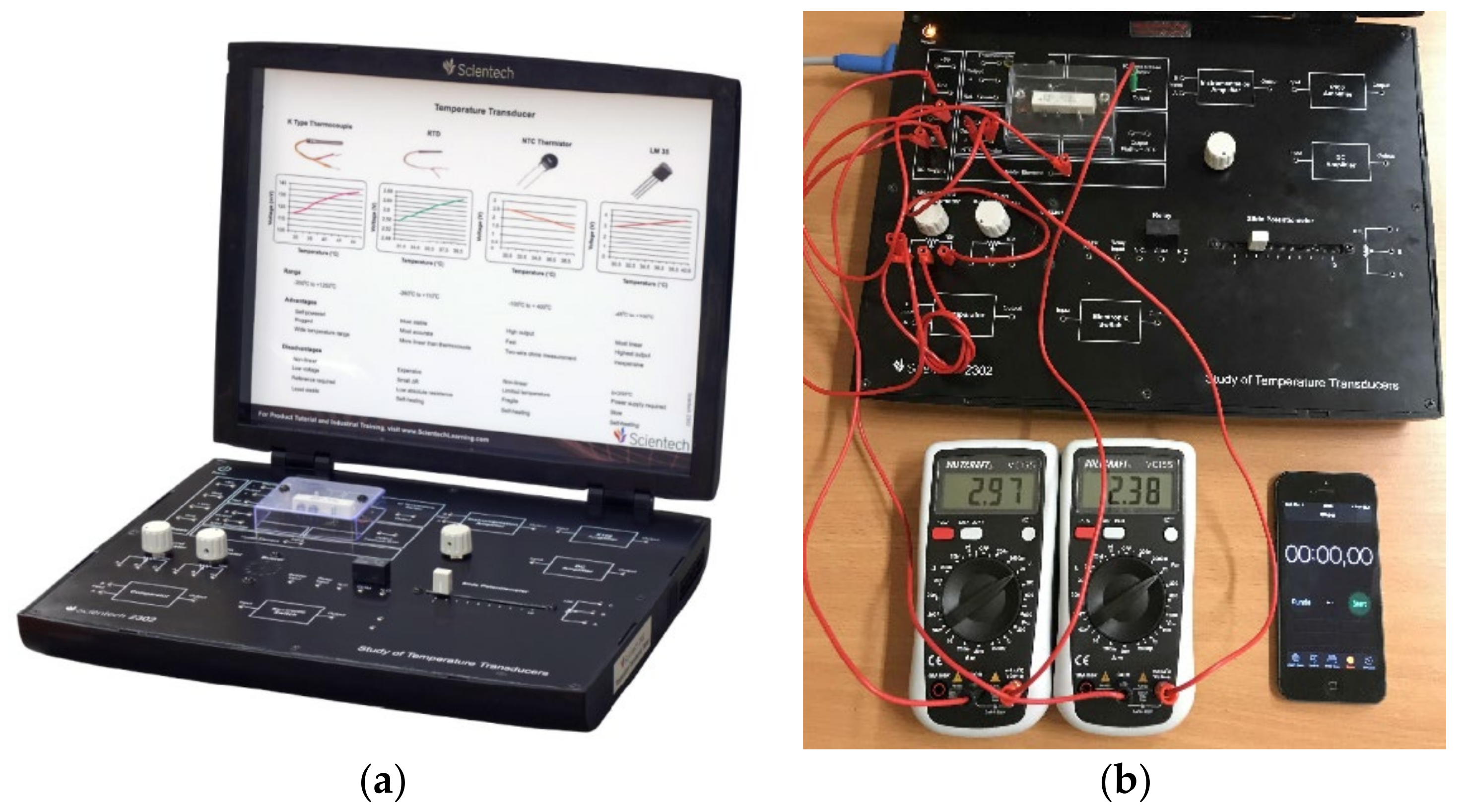
| Name of the Device | Type | Operating Conditions | Manufacturer |
|---|---|---|---|
| Scientech 2302 TechBook, Study of Temperature Transducers | Scientech 2302 | 0–40 °C 85% Rh | Scientech Technologies |
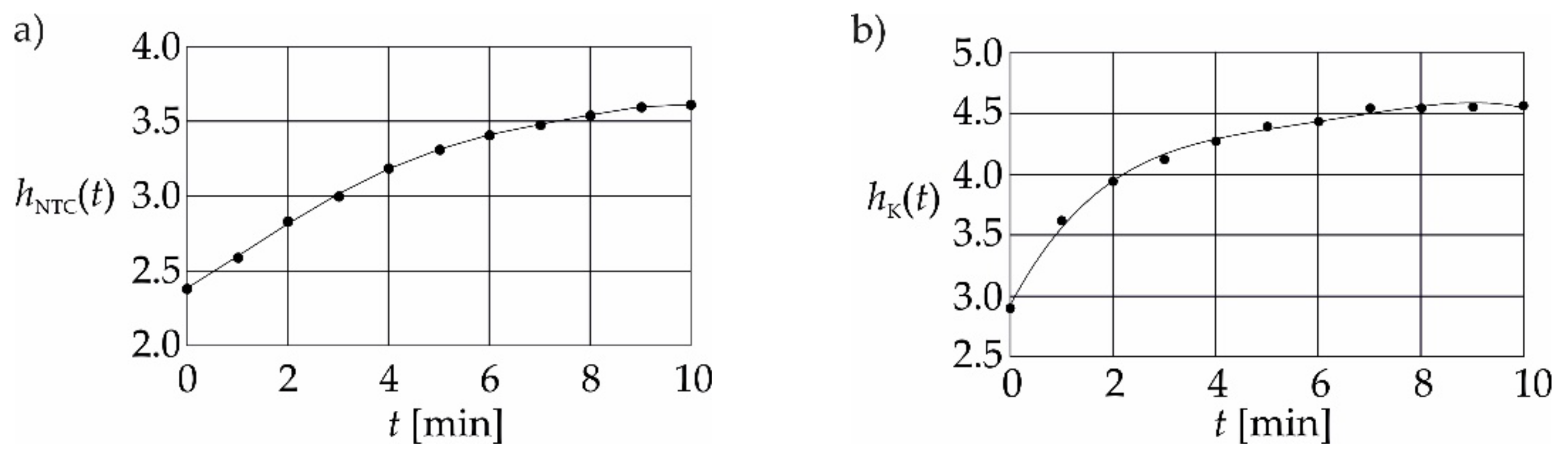
| Negative Temperature Coefficient (NTC) Sensor | |||||||||||
|---|---|---|---|---|---|---|---|---|---|---|---|
| t (min) | 0 | 1 | 2 | 3 | 4 | 5 | 6 | 7 | 8 | 9 | 10 |
| VNTC (V) | 2.38 | 2.59 | 2.83 | 3.00 | 3.19 | 3.31 | 3.41 | 3.48 | 3.54 | 3.60 | 3.61 |
| K-type Thermocouple Sensor | |||||||||||
| t (min) | 0 | 1 | 2 | 3 | 4 | 5 | 6 | 7 | 8 | 9 | 10 |
| VK (mV) | 2.90 | 3.62 | 3.94 | 4.12 | 4.27 | 4.39 | 4.43 | 4.54 | 4.54 | 4.55 | 4.56 |
Publisher’s Note: MDPI stays neutral with regard to jurisdictional claims in published maps and institutional affiliations. |
© 2022 by the authors. Licensee MDPI, Basel, Switzerland. This article is an open access article distributed under the terms and conditions of the Creative Commons Attribution (CC BY) license (https://creativecommons.org/licenses/by/4.0/).
Share and Cite
Tomczyk, K.; Beńko, P. Analysis of the Upper Bound of Dynamic Error Obtained during Temperature Measurements. Energies 2022, 15, 7300. https://doi.org/10.3390/en15197300
Tomczyk K, Beńko P. Analysis of the Upper Bound of Dynamic Error Obtained during Temperature Measurements. Energies. 2022; 15(19):7300. https://doi.org/10.3390/en15197300
Chicago/Turabian StyleTomczyk, Krzysztof, and Piotr Beńko. 2022. "Analysis of the Upper Bound of Dynamic Error Obtained during Temperature Measurements" Energies 15, no. 19: 7300. https://doi.org/10.3390/en15197300
APA StyleTomczyk, K., & Beńko, P. (2022). Analysis of the Upper Bound of Dynamic Error Obtained during Temperature Measurements. Energies, 15(19), 7300. https://doi.org/10.3390/en15197300