Output-Feedback Multi-Loop Positioning Technique via Dual Motor Synchronization Approach for Elevator System Applications

Abstract

This paper devises an output-feedback multi-loop positioning technique adopting the speed observer and multi-motor synchronizer, targeting the dual (master and slave) motor elevator system applications, providing the three contributions. First, the order-reduction observer continuously extracts the speed information from the motor position measurement, independent of the system model information. Second, the order-reduction stabilizer accomplishes the speed synchronization tasks for both the master and slave motors. Third, the resultant feedback system guarantees to exponentially recover the desired first-order transfer function from the reference to the actual motor position despite the model-plant mismatches. The prototype elevator system adopting the dual motor experimentally validates the practical advantages of the proposed technique.

1. Introduction

The ride comfort and dynamic performance of elevator systems greatly depend on their hardware (motor configuration) and software traction mechanism (feedback software structure with its tuning result). The main traction motor solely accomplished the pivotal positioning task for the passenger cart, requiring the high-power mechanical and electrical specification [1,2,3,4,5]. The multi-motor actuation systems have been recently adopted for large power applications due to the practical benefits, such as fault tolerance and power load reduction to the master motor (e.g., tug-of-war) [6,7,8,9]. This advanced system forming the master-slave motoring structure requires high-precision speed synchronization technology to improve both the positioning performance and rapid power distribution capability between the master and slave motors.

The conventional multi-loop proportional-integral (PI) controller for each master and slave motor enables us to address the positioning and speed synchronization problems simultaneously with the simple implementation [10]. The corresponding feedback gains were founded to satisfy the time or frequency domain specification via an ad hoc process and Bode/Nyquist plots for a fixed load condition. Thus, the operating condition changes in the actual applications raise the performance inconsistency problem due to the load and motor parameter variations. The gain scheduler including the database of multiple PI gains data would be considered as a solution to this problem, incorporating the additional computational complexity in the controller [11,12].

The pole-zero cancellation PI control partially alleviated this problem by constraining the feedback gain structure and including feed-forward terms, assigning the first-order closed-loop transfer function to each loop. However, this required the exact passive damping, rotor inertia, and stator inductance information to guarantee this benefit [10]. The recent parameter identification technologies could be adopted to address this practical challenging point, requiring the extra numerous dynamics and tuning factors for the adaptation process in the controller indirectly [13,14,15]. The nonlinear adaptive controls directly performed the parameter estimation tasks to accomplish the main mission of closed-loop stabilization by solving an optimization problem subject to the linear matrix constraints [16,17,18]. A similar adaptive controller solved the same serving problem through the integral back-stepping technique (multi-variable approach) whose closed-loop design and analysis tasks incorporated the complicated numerous matrix algebra [17]. There were passivity-based controllers including the disturbance observers (DOBs) for each loop and interesting online auto-tuning mechanisms while avoiding the matrix equality/inequality analysis processes [19,20]. The active disturbance rejection controls enlarged the feasible operating regions and improved the closed-loop performance, incorporating the state observer and DOBs estimating the lumped disturbances [21,22].

The extant solutions from the literature survey above leave the technical challenging points needed to be addressed as follows: (C1) the performance inconsistency depending on the operating conditions, (C2) the requirement of online parameter identifier to ensure the closed-loop stability and beneficial properties, and (C3) the involvement of the complicated matrix calculation process to tune the closed-loop performance. This study proposes an advanced and simple solution for the industrial elevator systems adopting the multi-motor by handling the challenging points C1–C3 whose contributions are recapitulated as:

• The design of the speed observer makes it possible to derive the output-feedback multi-loop solution invoking the order reduction by the specially designed gain structure, independent from any model and load information;
• The observer-based order-reduction speed stabilization technique results in both the pivotal inner loop for the positioning system (master motor) and the speed synchronizer (slave motor) through the specially designed gain structure and the combination of the integrator and DOB;
• The proof of the exponential convergence property recovering the desired first-order positioning performance by specifying the admissible ranges of design factors.

The experimental setup adopting the two 80-W BLDCMs and 32-bit digital signal processor (DSP) demonstrates the improved positioning and speed synchronization performances from the beneficial properties proved by the rigorous closed-loop analysis.

2. System Model

This study considers the DC servo system (including DCMs and BLDCMs) to demonstrate the main idea of the proposed solution as clearly as possible. The DC servo system has two mechanical and one electrical variable as the states given by $\theta \left(t\right)$ (rotor position in rad), $\omega \left(t\right)$ (rotor speed in rad/s), $i_a\left(t\right)$ (stator current in A) triggered by the control input $v_a\left(t\right)$ (stator voltage in V), which satisfies the dynamical relationships:

$$\begin{array}{ccc}\hfill \frac{d\theta \left(t\right)}{dt}& =& \omega \left(t\right),\hfill \end{array}$$

(1)

$$\begin{array}{ccc}\hfill J\frac{d\omega \left(t\right)}{dt}& =& -B\omega \left(t\right)+T_e\left(t\right)-T_L\left(t\right),\hfill \end{array}$$

(2)

$$\begin{array}{ccc}\hfill L_a\frac{d{i}_a\left(t\right)}{dt}& =& -R_a{i}_a\left(t\right)-{\varphi }_a\left(t\right)+v_a\left(t\right),\forall t\ge 0,\hfill \end{array}$$

(3)

where the output torque $T_e\left(t\right):=k_T{i}_a\left(t\right)$ (Nm) with $k_T>0$ representing the torque coefficient causes the rotational motion of the rotor position against the unknown load torque $T_L\left(t\right)$ (in Nm, acting as the matched disturbance). Another matched disturbance ${\varphi }_a\left(t\right)$ (back electromotive force (EMF)) drops the stator voltage $v_a\left(t\right)$, proportional to the rotor speed such that ${\varphi }_a\left(t\right):=k_e\omega \left(t\right)$ (V) with $k_e>0$ denoting the back EMF coefficient. The remaining coefficients J (kg/m${}^2$), B (Nm/rad/s), $L_a$ (H), and $R_a$ ($\Omega$) represent the (rotor) inertia, viscous damping, (stator) inductance, and resistance, suffering the unknown dramatic variations from their known nominal values; for example, $J=\Delta J+J_0$ with nominal inertia $J_0$ and variation $\Delta J$.

The Equation (3) yields the static relationship between the stator current $i_a\left(t\right)$ and voltage $v_a\left(t\right)$ such that

$$\begin{array}{c}\hfill i_a\left(t\right)=\frac{1}{R_a}\left(v_a\left(t\right)-k_e\omega \left(t\right)-L_a\frac{d{i}_a\left(t\right)}{dt}\right),\end{array}$$

which results in another expression of the speed dynamics (2):

$$\begin{array}{c}\hfill c_{\omega }\frac{d\omega \left(t\right)}{dt}=v_a\left(t\right)+d\left(t\right),\forall t\ge 0,\end{array}$$

(4)

where the known coefficient $c_{\omega }$ and unknown disturbance $d\left(t\right)$ are defined as $c_{\omega }:=\frac{J_0{R}_{a,0}}{k_{T,0}}$ and $d\left(t\right):=-(\frac{B{R}_a}{k_T}+k_e)\omega \left(t\right)-\frac{R_a}{k_T}{T}_L\left(t\right)-L_a\frac{d{i}_a\left(t\right)}{dt}-(\frac{J_0{R}_{a,0}}{k_{T,0}}-\frac{J{R}_a}{k_T})\frac{d\omega \left(t\right)}{dt}$. The resultant two dynamical Equations (5) and (6) simplify the master and slave servo system equations:

$$\begin{array}{ccc}\hfill \frac{d{\theta }_i\left(t\right)}{dt}& =& {\omega }_i\left(t\right),\hfill \end{array}$$

(5)

$$\begin{array}{ccc}\hfill c_{{\omega }_i}\frac{d{\omega }_i\left(t\right)}{dt}& =& v_{a,i}\left(t\right)+d_i\left(t\right),\forall t\ge 0,\hfill \end{array}$$

(6)

subject to the known coefficient $c_{{\omega }_i}$ (e.g., $c_{{\omega }_i}=\frac{J_{0,i}{R}_{a,0,i}}{k_{T,0,i}}$) and unknown time-varying disturbance $d_i\left(t\right)$ for each $i=1,2$ (1: master servo system, 2: slave servo system), which derives the proposed output-feedback solution, handling the three technical challenging points C1–C3. Figure 1 presents the elevator hardware configuration equipping the dual servo system.

3. Proposed Solution

3.1. Mission

For any position reference ${\theta }_{ref}$ ($={\mathcal{L}}^{-1}\left\{{\Theta }_{ref}\left(s\right)\right\}$, corresponding to the target elevator level), the desired position motion of the master servo system is denoted as ${\theta }_1^{*}\left(t\right)$ ($={\mathcal{L}}^{-1}\left\{{\Theta }_1^{*}\left(s\right)\right\}$), which defines the target closed-loop transfer function:

$$\begin{array}{c}\hfill \frac{{\Theta }_1^{*}\left(s\right)}{{\Theta }_{ref}\left(s\right)}=\frac{{\lambda }_{pc}}{s+{\lambda }_{pc}},\forall s\in \mathbb{C},\end{array}$$

(7)

subject to the cut-off frequency ${\lambda }_{pc}$ (rad/s, $f_{pc}=\frac{{\lambda }_{pc}}{2\pi }$ Hz). Then, the guarantee of exponential convergence (positioning)

$$\begin{array}{c}\hfill \underset{t\to \infty }{lim}{\theta }_1\left(t\right)={\theta }_1^{*}\left(t\right)\end{array}$$

(8)

renders the closed-loop system to rapidly recover the target performance (7), which is adopted as the main mission of the master motor. The additional mission (exponential synchronization):

$$\begin{array}{c}\hfill \underset{t\to \infty }{lim}{\omega }_2\left(t\right)={\omega }_1\left(t\right),\end{array}$$

(9)

is assigned for the slave motor to reduce the required power level of the master motor through the injection of the additional output torque of the slave motor to the closed-loop system. Therefore, it is desirable to shorten the transient period for the exponential synchronization (9), independent from the operating conditions.

3.2. Speed Observer

The motor position ${\theta }_i\left(t\right)$ evidently satisfies the relationship $\frac{d{\theta }_i\left(t\right)}{dt}={\omega }_i\left(t\right)$ and $\frac{d{\omega }_i\left(t\right)}{dt}=d_{o,i}\left(t\right)$ where ${\omega }_i\left(t\right)={\omega }_{i,0}\left(\mathrm{DC\; component}\right)+\Delta {\omega }_i\left(t\right)\left(\mathrm{AC\; component}\right)$ and $d_{o,i}\left(t\right):=\frac{d\Delta {\omega }_i\left(t\right)}{dt}$ ($|d_{o,i}\left(t\right)|\le {\overline{d}}_{o,i}$, $\forall t\ge 0$), yielding the observable linear system for ${\mathbf{x}}_i\left(t\right):={\left[\begin{array}{cc}{\theta }_i\left(t\right)& {\omega }_i\left(t\right)\end{array}\right]}^T$:

$$\begin{array}{c}\hfill \frac{d{\mathbf{x}}_i\left(t\right)}{dt}={\mathbf{A}}_o{\mathbf{x}}_i\left(t\right)+{\mathbf{b}}_o{d}_{o,i}\left(t\right),{\theta }_i\left(t\right)={\mathbf{c}}_o^T{\mathbf{x}}_i\left(t\right),\forall t\ge 0,\end{array}$$

(10)

where ${\mathbf{b}}_o:=\left[\begin{array}{c}0\\ 1\end{array}\right]$, ${\mathbf{A}}_o:=\left[\begin{array}{cc}0& 1\\ 0& 0\end{array}\right]$, and ${\mathbf{c}}_o:=\left[\begin{array}{c}1\\ 0\end{array}\right]$, which satisfies for $\mathbb{O}=\left[\begin{array}{c}{\mathbf{c}}_o^T\\ {\mathbf{c}}_o^T{\mathbf{A}}_o\end{array}\right]$ that rank$\left(\mathbb{O}\right)$ = rank $\left(\left[\begin{array}{cc}1& 0\\ 0& 1\end{array}\right]\right)=2$ (observability).

To handle the challenging points C2 and C3, this study suggests an advanced model-free solution by specifying the gain structure of the Luenberger-type observer such that

$$\begin{array}{c}\hfill \frac{d{\widehat{\mathbf{x}}}_i\left(t\right)}{dt}={\mathbf{A}}_o{\widehat{\mathbf{x}}}_i\left(t\right)+{\mathbf{l}}_{o,i}({\theta }_i\left(t\right)-{\widehat{\theta }}_i\left(t\right)),{\widehat{\theta }}_i\left(t\right)={\mathbf{c}}_o^T{\widehat{\mathbf{x}}}_i\left(t\right),i=1,2,\forall t\ge 0,\end{array}$$

(11)

where the two tuning factors ${\zeta }_{o,i}>0$ and ${\lambda }_{o,i}>0$ constitute the observer gain:

$$\begin{array}{c}\hfill {\mathbf{l}}_{o,i}=\left[\begin{array}{c}{l}_{o,i,1}\\ l_{o,i,2}\end{array}\right]:=\left[\begin{array}{c}{\zeta }_{o,i}+{\lambda }_{o,i}\\ {\zeta }_{o,i}{\lambda }_{o,i}\end{array}\right]\end{array}$$

(12)

which makes it possible to design an observer-based output-feedback system for each master and slave motor.

Remark 1.

The tuning factor ${\zeta }_{o,i}$ plays a role in attenuating the disturbance intensity $d_{o,i}\left(t\right)$ to ensure the first-order observer error dynamics for $e_{{\theta }_i}\left(t\right):={\theta }_i\left(t\right)-{\widehat{\theta }}_i\left(t\right)$ and $e_{{\omega }_i}\left(t\right):={\omega }_i\left(t\right)-{\widehat{\omega }}_i\left(t\right)$:

$$\begin{array}{c}\hfill \frac{d{e}_{{\theta }_i}\left(t\right)}{dt}=-{\lambda }_{o,i}{e}_{{\theta }_i}\left(t\right),\frac{d{e}_{{\omega }_i}\left(t\right)}{dt}=-{\lambda }_{o,i}{e}_{{\omega }_i}\left(t\right),\forall t\ge 0,\end{array}$$

by constraining ${\zeta }_{o,i}$ into some interval through the order-reduction property. See Section 4 for details.

3.3. Master Motor Output-Feedback System (for Positioning)

3.3.1. Outer Loop

The position dynamics of the master motor can be rewritten from (5) by extracting the design variable ${\omega }_0\left(t\right)$:

$$\begin{array}{c}\hfill \frac{d{\theta }_1\left(t\right)}{dt}={\omega }_1\left(t\right)={\omega }_0\left(t\right)-\Delta {\omega }_1\left(t\right),\forall t\ge 0,\end{array}$$

(13)

where $\Delta {\omega }_1\left(t\right):={\omega }_0\left(t\right)-{\omega }_1\left(t\right)$. This study chooses a simple feedback for ${\tilde{\theta }}_1\left(t\right):={\theta }_{ref}-{\theta }_1\left(t\right)$ as the update rule for ${\omega }_0\left(t\right)$:

$$\begin{array}{c}\hfill {\omega }_0\left(t\right)={\lambda }_{pc}{\tilde{\theta }}_1\left(t\right),\forall t\ge 0,\end{array}$$

(14)

resulting in the closed-loop outer loop (by combining (14) and (13)):

$$\begin{array}{c}\hfill \frac{d{\theta }_1\left(t\right)}{dt}={\lambda }_{pc}{\tilde{\theta }}_1\left(t\right)-\Delta {\omega }_1\left(t\right),\forall t\ge 0.\end{array}$$

(15)

The controlled system (15) accomplishes the main mission (8) (e.g., the exponential convergence ${lim}_{t\to \infty }{\theta }_1\left(t\right)={\theta }_1^{*}\left(t\right)$), provided that

$$\begin{array}{c}\hfill \underset{t\to \infty }{lim}\Delta {\omega }_1\left(t\right)=0\end{array}$$

exponentially, which is adopted as the primary mission for the inner loop in the following section.

3.3.2. Inner Loop

The open-loop system (6), second subsystem of the observer (11), and control (14) yield the open-loop dynamics for the estimated error $\Delta {\widehat{\omega }}_1\left(t\right):={\omega }_0\left(t\right)-{\widehat{\omega }}_1\left(t\right)$ as

$$\begin{array}{ccc}\hfill c_{{\omega }_1}\frac{d\Delta {\widehat{\omega }}_1\left(t\right)}{dt}& =& c_{{\omega }_1}\frac{d{\omega }_0\left(t\right)}{dt}-c_{{\omega }_1}\frac{d{\widehat{\omega }}_1\left(t\right)}{dt}+c_{{\omega }_1}\frac{d{\omega }_1\left(t\right)}{dt}-c_{{\omega }_1}\frac{d{\omega }_1\left(t\right)}{dt}\hfill \\ & =& -v_{a,1}\left(t\right)-c_{{\omega }_1}{\lambda }_{pc}{\omega }_1\left(t\right)-d_1\left(t\right)+c_{{\omega }_1}\frac{d{e}_{{\omega }_1}\left(t\right)}{dt},\hfill \end{array}$$

(16)

whose stabilization action for the stator voltage $v_{a,1}\left(t\right)$ is suggested as

$$\begin{array}{c}\hfill v_{a,1}\left(t\right)=k_{P,{\omega }_1}\Delta {\widehat{\omega }}_1\left(t\right)+k_{I,{\omega }_1}{\int }_0^t\Delta {\widehat{\omega }}_1\left(\tau \right)d\tau -c_{{\omega }_1}{\lambda }_{pc}{\widehat{\omega }}_1\left(t\right)-{\widehat{d}}_1\left(t\right),\end{array}$$

(17)

where ${\zeta }_{{\omega }_1}>0$ and ${\lambda }_{{\omega }_1}>0$ constitute the feedback gains $k_{P,{\omega }_1}$ and $k_{I,{\omega }_1}$:

$$\begin{array}{c}\hfill k_{P,{\omega }_1}:={\zeta }_{{\omega }_1}+c_{{\omega }_1}{\lambda }_{{\omega }_1},k_{I,{\omega }_1}:={\zeta }_{{\omega }_1}{\lambda }_{{\omega }_1}.\end{array}$$

(18)

The observer-based DOB driven by the state variable $z_{d_1}\left(t\right)$ obtains the estimated disturbance ${\widehat{d}}_1\left(t\right)$ as its output such that

$$\begin{array}{ccc}\hfill \frac{d{z}_{d_1}\left(t\right)}{dt}& =& -l_{d_1}{z}_{d_1}\left(t\right)+l_{d_1}^2{c}_{{\omega }_1}\Delta {\widehat{\omega }}_1\left(t\right)+l_{d_1}{\widehat{p}}_{{\omega }_1}\left(t\right),\hfill \end{array}$$

(19)

$$\begin{array}{ccc}\hfill {\widehat{d}}_1\left(t\right)& =& z_{d_1}\left(t\right)-l_{d_1}{c}_{{\omega }_1}\Delta {\widehat{\omega }}_1\left(t\right),\forall t\ge 0,\hfill \end{array}$$

(20)

subject to the gain $l_{d_1}>0$ with the estimated signal ${\widehat{p}}_{{\omega }_1}\left(t\right)$ for the actual signal $p_{{\omega }_1}\left(t\right)$ defined as $p_{{\omega }_1}\left(t\right):=-v_{a,1}\left(t\right)-c_{{\omega }_1}{\lambda }_{pc}{\omega }_1\left(t\right)$ and ${\widehat{p}}_{{\omega }_1}\left(t\right):=p_{{\omega }_1}\left(t\right){|}_{{\omega }_1\left(t\right)={\widehat{\omega }}_1\left(t\right)}$ (e.g., ${\widehat{p}}_{{\omega }_1}\left(t\right)=-v_{a,1}\left(t\right)-c_{{\omega }_1}{\lambda }_{pc}{\widehat{\omega }}_1\left(t\right)$). The proposed solution (17) results in the controlled system (by substituting (17) to the open-loop dynamics (16))

$$\begin{array}{ccc}\hfill c_{{\omega }_1}\frac{d\Delta {\widehat{\omega }}_1\left(t\right)}{dt}& =& -k_{P,{\omega }_1}\Delta {\widehat{\omega }}_1\left(t\right)-k_{I,{\omega }_1}{\int }_0^t\Delta {\widehat{\omega }}_1\left(\tau \right)d\tau -c_{{\omega }_1}{\lambda }_{pc}{e}_{{\omega }_1}\left(t\right)-e_{d_1}\left(t\right)\hfill \\ & & +c_{{\omega }_1}\frac{d{e}_{{\omega }_1}\left(t\right)}{dt},\hfill \end{array}$$

(21)

where $e_{d_1}\left(t\right):=d_1\left(t\right)-{\widehat{d}}_1\left(t\right)$, whose properties are analyzed in Section 4.

Remark 2.

The introductions of the specially structured feedback gains (18) and observer-based DOB (19) and (20) address the challenging points C1–C3. Specifically, the tuning factor ${\zeta }_{{\omega }_1}$ plays a role in attenuating the disturbance intensity $d_1\left(t\right)$ to ensure the first-order dynamics for the actual error $\Delta {\omega }_1\left(t\right)={\omega }_0\left(t\right)-{\omega }_1\left(t\right)$:

$$\begin{array}{c}\hfill \frac{d\Delta {\omega }_1\left(t\right)}{dt}=-{\lambda }_{{\omega }_1}\Delta {\omega }_1\left(t\right),\forall t\ge 0,\end{array}$$

by constraining ${\zeta }_{{\omega }_1}$ into some interval through the order-reduction property. See Section 4 for details.

3.4. Slave Motor Output-Feedback System (for Speed Synchronization)

The open-loop system (6) and second subsystem of the observer (11) yield the open-loop dynamics for the estimated synchronization error $\Delta {\widehat{\omega }}_2\left(t\right):={\widehat{\omega }}_1\left(t\right)-{\widehat{\omega }}_2\left(t\right)$ as

$$\begin{array}{ccc}\hfill c_{{\omega }_2}\frac{d\Delta {\widehat{\omega }}_2\left(t\right)}{dt}& =& c_{{\omega }_2}\frac{d{\widehat{\omega }}_1\left(t\right)}{dt}-c_{{\omega }_2}\frac{d{\widehat{\omega }}_2\left(t\right)}{dt}+c_{{\omega }_2}\frac{d{\omega }_2\left(t\right)}{dt}-c_{{\omega }_2}\frac{d{\omega }_2\left(t\right)}{dt}\hfill \\ & =& -v_{a,2}\left(t\right)+c_{{\omega }_2}{l}_{o,1,2}{e}_{{\theta }_1}\left(t\right)-d_2\left(t\right)+c_{{\omega }_2}\frac{d{e}_{{\omega }_2}\left(t\right)}{dt},\hfill \end{array}$$

(22)

whose stabilization action for the stator voltage $v_{a,2}\left(t\right)$ is suggested as

$$\begin{array}{c}\hfill v_{a,2}\left(t\right)=k_{P,{\omega }_2}\Delta {\widehat{\omega }}_2\left(t\right)+k_{I,{\omega }_2}{\int }_0^t\Delta {\widehat{\omega }}_2\left(\tau \right)d\tau +c_{{\omega }_2}{l}_{o,1,2}{e}_{{\theta }_1}\left(t\right)-{\widehat{d}}_2\left(t\right),\end{array}$$

(23)

where the two tuning factors ${\zeta }_{{\omega }_2}>0$ and ${\lambda }_{{\omega }_2}>0$ constitute the feedback gains $k_{P,{\omega }_2}$ and $k_{I,{\omega }_2}$:

$$\begin{array}{c}\hfill k_{P,{\omega }_2}:={\zeta }_{{\omega }_2}+c_{{\omega }_2}{\lambda }_{{\omega }_2},k_{I,{\omega }_2}:={\zeta }_{{\omega }_2}{\lambda }_{{\omega }_2}.\end{array}$$

(24)

The observer-based DOB driven by the state variable $z_{d_2}\left(t\right)$ obtains the estimated disturbance ${\widehat{d}}_2\left(t\right)$ as its output such that

$$\begin{array}{ccc}\hfill \frac{d{z}_{d_2}\left(t\right)}{dt}& =& -l_{d_2}{z}_{d_2}\left(t\right)+l_{d_2}^2{c}_{{\omega }_2}\Delta {\widehat{\omega }}_2\left(t\right)+l_{d_2}{p}_{{\omega }_2}\left(t\right),\hfill \end{array}$$

(25)

$$\begin{array}{ccc}\hfill {\widehat{d}}_2\left(t\right)& =& z_{d_2}\left(t\right)-l_{d_2}{c}_{{\omega }_2}\Delta {\widehat{\omega }}_2\left(t\right),\forall t\ge 0,\hfill \end{array}$$

(26)

subject to the gain $l_{d_2}>0$ with the estimated signal ${\widehat{p}}_{{\omega }_2}\left(t\right)$ for the actual signal $p_{{\omega }_2}\left(t\right)$ defined as $p_{{\omega }_2}\left(t\right):=-v_{a,2}\left(t\right)+c_{{\omega }_2}{l}_{o,1,2}{e}_{{\theta }_1}\left(t\right)$. The proposed solution (23) results in the controlled system as (by substituting (23) to the open-loop dynamics (22))

$$\begin{array}{c}\hfill c_{{\omega }_2}\frac{d\Delta {\widehat{\omega }}_2\left(t\right)}{dt}=-k_{P,{\omega }_2}\Delta {\widehat{\omega }}_2\left(t\right)-k_{I,{\omega }_2}{\int }_0^t\Delta {\widehat{\omega }}_2\left(\tau \right)d\tau -e_{d_2}\left(t\right)+c_{{\omega }_2}\frac{d{e}_{{\omega }_2}\left(t\right)}{dt},\end{array}$$

(27)

where $e_{d_2}\left(t\right):=d_2\left(t\right)-{\widehat{d}}_2\left(t\right)$, whose properties are analyzed in Section 4. Figure 2 illustrates the proposed multi-loop positioning system including the speed synchronizer for master and slave motor where $p_{ref}$ denotes the floor command of the elevator system (e.g., $p_{ref}\in \{B_N,\cdots ,B_2,B_1,1,2,\cdots ,N\}$). Figure 3 summarizes the design factors of the proposed solution.

Remark 3.

The introductions of the specially structured feedback gains (24) and observer-based DOB (25) and (20) addresses the challenging points C1–C3. Specifically, the tuning factor ${\zeta }_{{\omega }_2}$ plays a role in attenuating the disturbance intensity $d_2\left(t\right)$ to ensure the first-order dynamics for the actual synchronization error $\Delta {\omega }_2\left(t\right):={\omega }_1\left(t\right)-{\omega }_2\left(t\right)$:

$$\begin{array}{c}\hfill \frac{d\Delta {\omega }_2\left(t\right)}{dt}=-{\lambda }_{{\omega }_2}\Delta {\omega }_2\left(t\right),\forall t\ge 0,\end{array}$$

by constraining ${\zeta }_{{\omega }_2}$ into some interval through the order-reduction property. See Section 4 for details.

4. Analysis

This section checks whether the proposed multi-loop system with speed synchronization accomplishes the main mission (8) (in Section 4.2) and additional mission (9) (in Section 4.3). To this end, Section 4.1 begins with the analysis of the auxiliary systems, such as observer and DOB used for both the master and slave motors, where $\dot{f}\left(t\right)$ represents the time derivative operation on $f\left(t\right)$ (e.g., $\dot{f}\left(t\right)=\frac{df\left(t\right)}{dt}$, $\forall t\ge 0$). Note that all the proofs of the analysis results are included in the Appendix A.

4.1. Auxiliary Systems for Master and Slave Motors

4.1.1. Observer

Lemma 1 derives the first-order output error dynamics of the observer obtained from the order-reduction property triggered by the specially designed gain structure.

Lemma 1.

The observer output error $e_{{\theta }_i}\left(t\right)$ from (11) and (12) satisfies

$$\begin{array}{c}\hfill {\dot{e}}_{{\theta }_i}\left(t\right)=-{\lambda }_{o,i}{e}_{{\theta }_i}\left(t\right)+x_{o,i}\left(t\right)\end{array}$$

(28)

with $x_{o,i}\left(t\right)$ denoting the perturbation from the system

$$\begin{array}{c}\hfill {\dot{x}}_{o,i}\left(t\right)=-{\zeta }_{o,i}{x}_{o,i}\left(t\right)+d_{o,i}\left(t\right),\forall t\ge 0.\end{array}$$

(29)

Lemma 2 specifies the admissible range for the design factor ${\zeta }_{o,i}$ constraining the output error dynamics (28) into its desired version (31).

Lemma 2.

The choice for ${\zeta }_{o,i}$ such that $\frac{2{\overline{d}}_{o,i}}{{\zeta }_{o,i}}\approx 0$ ensures the exponential convergence

$$\begin{array}{c}\hfill \underset{t\to \infty }{lim}{e}_{{\theta }_i}\left(t\right)=e_{{\theta }_i}^{*}\left(t\right)\end{array}$$

(30)

for the system

$$\begin{array}{c}\hfill {\dot{e}}_{{\theta }_i}^{*}\left(t\right)=-{\lambda }_{o,i}{e}_{{\theta }_i}^{*}\left(t\right),\forall t\ge 0.\end{array}$$

(31)

Remark 4.

The result (30) showing $|e_{{\theta }_i}^{*}-e_{{\theta }_i}|\approx 0$ provides a rationale to use the equation (by combining (30) and (31)):

$$\begin{array}{c}\hfill {\dot{e}}_{{\theta }_i}=-{\lambda }_{o,i}{e}_{{\theta }_i}\end{array}$$

which implies the chain reasoning tasks such that (based on (11))

$$\begin{array}{ccc}\hfill {\ddot{e}}_{{\theta }_i}=-{\lambda }_{o,i}{\dot{e}}_{{\theta }_i}& \iff & {\ddot{\theta }}_i-{\ddot{\widehat{\theta }}}_i=-{\lambda }_{o,i}({\dot{\theta }}_i-{\dot{\widehat{\theta }}}_i)\hfill \\ & \iff & {\dot{\omega }}_i-(l_{o,i,1}{\dot{e}}_{{\theta }_i}+{\dot{\widehat{\omega }}}_i)=-{\lambda }_{o,i}({\omega }_i-(l_{o,i,1}{e}_{{\theta }_i}+{\widehat{\omega }}_i))\hfill \\ & \iff & {\dot{e}}_{{\omega }_i}+{\lambda }_{o,i}{l}_{o,i,1}{e}_{{\theta }_i}=-{\lambda }_{o,i}{e}_{{\omega }_i}+{\lambda }_o{l}_{o,i,1}{e}_{{\theta }_i},\hfill \end{array}$$

concluding

$$\begin{array}{c}\hfill {\dot{\mathit{e}}}_{o,i}=-{\lambda }_{o,i}{\mathit{e}}_{o,i},\forall t\ge 0,\end{array}$$

(32)

for some range of ${\zeta }_{o,i}>0$ where ${\mathit{e}}_{o,i}={\left[\begin{array}{cc}{e}_{{\theta }_i}& e_{{\omega }_i}\end{array}\right]}^T$, which is the main message of this subsection.

4.1.2. DOB

Lemma 3 derives the disturbance estimation error dynamics for $e_{d_i}\left(t\right)=d_i-{\widehat{d}}_i$ ($i=1,2$) by further examining the DOB dynamics (19) and (25) and its outputs (20) and (26).

Lemma 3.

The output error $e_{d_i}\left(t\right)$ driven by the DOBs (19) and (20) for master motor and (25) and (26) for slave motor satisfies

$$\begin{array}{c}\hfill {\dot{e}}_{d_i}\left(t\right)=-l_{d_i}{e}_{d_i}\left(t\right)+{\mathit{q}}_{d_i}^T{\mathit{e}}_{o,i}\left(t\right)+f_{d_i}\left(t\right)\end{array}$$

(33)

for some ${\mathit{q}}_{d_i}\in {\mathbb{R}}^2$ where $f_{d_i}\left(t\right):={\dot{d}}_i\left(t\right)$ and $|f_{d_i}\left(t\right)|\le {\overline{f}}_{d_i}$, $i=1,2$, $\forall t\ge 0$.

Remark 5.

The setting $e_{{\omega }_i}\approx 0$ (by (32)) for the result (33) leads to the system ${\dot{\widehat{d}}}_i=l_{d_i}(d_i-{\widehat{d}}_i)$ showing

$$\begin{array}{c}\hfill \frac{{\widehat{D}}_i\left(s\right)}{D_i\left(s\right)}=\frac{l_{d_i}}{s+l_{d_i}},\forall s\in \mathbb{C},\end{array}$$

(34)

where $D_i\left(s\right)=\mathcal{L}\left\{d_i\right\}$ and ${\widehat{D}}_i\left(s\right)=\mathcal{L}\left\{{\widehat{d}}_i\right\}$, suggesting for the design factor $l_{d_i}$ tuned as the cut-off frequency of the transfer function (34) (e.g., $l_{d_i}$ rad/s or, equivalently, $f_{d_i}=\frac{l_{d_i}}{2\pi }$ Hz).

4.2. Multi-Loop Positioning System for Master Motor

Using the analysis results of Section 4.1, this subsection proves the accomplishment of the main mission (8) by analyzing the inner (Section 4.2.1) and entire loop (Section 4.2.2) sequentially.

4.2.1. Inner Loop

Lemma 4 derives the first-order estimated speed error dynamics for $\Delta {\widehat{\omega }}_1\left(t\right)={\omega }_0\left(t\right)-{\widehat{\omega }}_1\left(t\right)$ obtained from the order-reduction property triggered by the specially designed gain structure.

Lemma 4.

The estimated error $\Delta {\widehat{\omega }}_1\left(t\right)$ driven by the control law (17) and its gain (18) satisfies

$$\begin{array}{c}\hfill \Delta {\dot{\widehat{\omega }}}_1\left(t\right)=-{\lambda }_{{\omega }_1}\Delta {\widehat{\omega }}_1\left(t\right)-\frac{1}{c_{{\omega }_1}}{x}_{{\omega }_1}\left(t\right)+\frac{1}{c_{{\omega }_1}}{e}_1\left(t\right)\end{array}$$

(35)

and its filtered version such that

$$\begin{array}{c}\hfill {\dot{x}}_{{\omega }_1}\left(t\right)=-\frac{{\zeta }_{{\omega }_1}}{c_{{\omega }_1}}{x}_{{\omega }_1}\left(t\right)+\frac{{\zeta }_{{\omega }_1}}{c_{{\omega }_1}}{e}_1\left(t\right)\end{array}$$

(36)

where $e_1\left(t\right):=-e_{d_1}\left(t\right)-c_{{\omega }_1}({\lambda }_{pc}+{\lambda }_{o,1})e_{{\omega }_1}\left(t\right)$, $\forall t\ge 0$.

Theorem 1 specifies the admissible range for the design factor $l_{d_1}$ constraining the estimated speed error dynamics (35) for $\Delta {\widehat{\omega }}_1\left(t\right)$ into its desired version (38).

Theorem 1.

The choice for $l_{d_1}$ such that $\frac{2{\overline{f}}_{d_1}}{l_{d_1}}\approx 0$ ensures the exponential convergence

$$\begin{array}{c}\hfill \underset{t\to \infty }{lim}\Delta {\widehat{\omega }}_1\left(t\right)=\Delta {\omega }_1^{*}\left(t\right)\end{array}$$

(37)

for the system

$$\begin{array}{c}\hfill \Delta {\dot{\omega }}_1^{*}\left(t\right)=-{\lambda }_{{\omega }_1}\Delta {\omega }_1^{*}\left(t\right),\forall t\ge 0.\end{array}$$

(38)

Remark 6.

The result (37) showing $|\Delta {\omega }_1^{*}-\Delta {\widehat{\omega }}_1|\approx 0$ provides a rationale to use the equation (by combining (37) and (38)):

$$\begin{array}{c}\hfill \Delta {\dot{\widehat{\omega }}}_1=-{\lambda }_{{\omega }_1}\Delta {\widehat{\omega }}_1,\forall t\ge 0,\end{array}$$

equivalently,

$$\begin{array}{c}\hfill \Delta {\dot{\omega }}_1=-{\lambda }_{{\omega }_1}\Delta {\omega }_1+{\mathit{q}}_{{\omega }_1}^T{\mathit{e}}_{o,1}\end{array}$$

(39)

for some range of $l_{d_1}>0$ where ${\mathit{q}}_{{\omega }_1}:={\left[\begin{array}{cc}0& {\lambda }_{o,1}-{\lambda }_{{\omega }_1}\end{array}\right]}^T$, which renders the positive definite function $V_{\Delta {\omega }_1}:=\frac{1}{2}\Delta {\omega }_1^2+\frac{{\eta }_{{\omega }_1}}{2}{\parallel {\mathit{e}}_{o,1}\parallel }^2$, ${\eta }_{{\omega }_1}>0$, to be

$$\begin{array}{ccc}\hfill {\dot{V}}_{\Delta {\omega }_1}& =& \Delta {\omega }_1(-{\lambda }_{{\omega }_1}\Delta {\omega }_1+{\mathit{q}}_{{\omega }_1}^T{\mathit{e}}_{o,1})-{\eta }_{{\omega }_1}{\lambda }_{o,1}{\parallel {\mathit{e}}_{o,1}\parallel }^2\hfill \\ & \le & -\frac{{\lambda }_{{\omega }_1}}{2}\Delta {\omega }_1^2-({\eta }_{{\omega }_1}{\lambda }_{o,1}-\frac{\parallel {\mathit{q}}_{{\omega }_1}{\parallel }^2}{2{\lambda }_{{\omega }_1}}){\parallel {\mathit{e}}_{o,1}\parallel }^2,\forall t\ge 0.\hfill \end{array}$$

Thus, the choice of ${\eta }_{{\omega }_1}=\frac{1}{{\lambda }_{o,1}}(\frac{\parallel {\mathit{q}}_{{\omega }_1}{\parallel }^2}{2{\lambda }_{{\omega }_1}}+\frac{1}{2})$ concludes this section with the inequality:

$$\begin{array}{c}\hfill {\dot{V}}_{\Delta {\omega }_1}\le -{\alpha }_{\Delta {\omega }_1}{V}_{\Delta {\omega }_1},\forall t\ge 0,\end{array}$$

(40)

where ${\alpha }_{\Delta {\omega }_1}=min\{{\lambda }_{{\omega }_1},\frac{1}{{\eta }_{{\omega }_1}}\}$, which is the main message of this subsection.

4.2.2. Entire Loop

Theorem 2 proves that the proposed solution depicted in Figure 2 attains the main mission (8) incorporating the inequality (40) obtained from Section 4.2.1 as its main message.

Theorem 2.

Under the same settings of Lemma 1 and Theorem 1, the master positioning system shown in Figure 2 accomplishes the main mission (8) (e.g., ensuring ${lim}_{t\to \infty }{\theta }_1\left(t\right)={\theta }_1^{*}\left(t\right)$ exponentially).

4.3. Speed Synchronization System for Slave Motor

Using the analysis results of Section 4.1, this subsection proves the accomplishment of the additional mission (9) by analyzing the synchronization loop in a similar way to that used in Section 4.2.1. To this end, Lemma 4 derives the first-order estimated speed error dynamics for $\Delta {\widehat{\omega }}_2\left(t\right)={\widehat{\omega }}_1\left(t\right)-{\widehat{\omega }}_2\left(t\right)$ obtained from the order-reduction property triggered by the specially designed gain structure.

Lemma 5.

The estimated error $\Delta {\widehat{\omega }}_2\left(t\right)$ driven by the control law (23) and its gain (24) satisfies

$$\begin{array}{c}\hfill \Delta {\dot{\widehat{\omega }}}_2\left(t\right)=-{\lambda }_{{\omega }_2}\Delta {\widehat{\omega }}_2\left(t\right)-\frac{1}{c_{{\omega }_2}}{x}_{{\omega }_2}\left(t\right)+\frac{1}{c_{{\omega }_2}}{e}_2\left(t\right)\end{array}$$

(41)

and its filtered version such that

$$\begin{array}{c}\hfill {\dot{x}}_{{\omega }_2}\left(t\right)=-\frac{{\zeta }_{{\omega }_2}}{c_{{\omega }_2}}{x}_{{\omega }_2}\left(t\right)+\frac{{\zeta }_{{\omega }_2}}{c_{{\omega }_2}}{e}_2\left(t\right)\end{array}$$

(42)

where $e_2\left(t\right):=-e_{d_2}\left(t\right)-c_{{\omega }_1}{\lambda }_{o,2}{e}_{{\omega }_2}\left(t\right)$, $\forall t\ge 0$.

Theorem 3 specifies the admissible range for the design factor $l_{d_2}$ constraining the estimated speed error dynamics (41) for $\Delta {\widehat{\omega }}_2\left(t\right)$ into its desired version (44).

Theorem 3.

The choice for $l_{d_2}$ such that $\frac{2{\overline{f}}_{d_2}}{l_{d_2}}\approx 0$ ensures the exponential convergence

$$\begin{array}{c}\hfill \underset{t\to \infty }{lim}\Delta {\widehat{\omega }}_2\left(t\right)=\Delta {\omega }_2^{*}\left(t\right)\end{array}$$

(43)

for the system

$$\begin{array}{c}\hfill \Delta {\dot{\omega }}_2^{*}\left(t\right)=-{\lambda }_{{\omega }_2}\Delta {\omega }_2^{*}\left(t\right),\forall t\ge 0.\end{array}$$

(44)

Remark 7.

The result (43) showing $|\Delta {\omega }_2^{*}-\Delta {\widehat{\omega }}_2|\approx 0$ provides a rationale to use the equation (by combining (43) and (44)):

$$\begin{array}{c}\hfill \Delta {\dot{\widehat{\omega }}}_2=-{\lambda }_{{\omega }_2}\Delta {\widehat{\omega }}_2,\forall t\ge 0,\end{array}$$

equivalently,

$$\begin{array}{c}\hfill \Delta {\dot{\omega }}_2=-{\lambda }_{{\omega }_2}\Delta {\omega }_2+\sum _{i=1}^2{\mathit{q}}_{{\omega }_i}^T{\mathit{e}}_{o,i}\end{array}$$

for some range of $l_{d_2}>0$ where ${\mathit{q}}_{{\omega }_1}:={\left[\begin{array}{cc}0& -({\lambda }_{o,1}-{\lambda }_{{\omega }_2})\end{array}\right]}^T$ and ${\mathit{q}}_{{\omega }_2}:={\left[\begin{array}{cc}0& {\lambda }_{o,2}-{\lambda }_{{\omega }_2}\end{array}\right]}^T$, which renders the positive definite function $V_{\Delta {\omega }_2}:=\frac{1}{2}\Delta {\omega }_2^2+{\sum }_{i=1}^2\frac{{\eta }_{{\omega }_{2,i}}}{2}{\parallel {\mathit{e}}_{o,i}\parallel }^2$, ${\eta }_{{\omega }_2,i}>0$ ($i=1,2$), to be

$$\begin{array}{ccc}\hfill {\dot{V}}_{\Delta {\omega }_2}& =& \Delta {\omega }_2(-{\lambda }_{{\omega }_2}\Delta {\omega }_2+\sum _{i=1}^2{\mathit{q}}_{{\omega }_i}^T{\mathit{e}}_{o,i})-\sum _{i=1}^2{\eta }_{{\omega }_{2,i}}{\lambda }_{o,i}{\parallel {\mathit{e}}_{o,i}\parallel }^2\hfill \\ & \le & -\frac{{\lambda }_{{\omega }_2}}{3}\Delta {\omega }_2^2-\sum _{i=1}^2({\eta }_{{\omega }_{2,i}}{\lambda }_{o,i}-\frac{3\parallel {\mathit{q}}_{{\omega }_i}{\parallel }^2}{4{\lambda }_{{\omega }_2}}){\parallel {\mathit{e}}_{o,i}\parallel }^2,\forall t\ge 0.\hfill \end{array}$$

Thus, the choice of ${\eta }_{{\omega }_{2,i}}=\frac{1}{{\lambda }_{o,i}}(\frac{3\parallel {\mathit{q}}_{{\omega }_i}{\parallel }^2}{4{\lambda }_{{\omega }_2}}+\frac{1}{2})$ concludes this section with the inequality:

$$\begin{array}{c}\hfill {\dot{V}}_{\Delta {\omega }_2}\le -{\alpha }_{\Delta {\omega }_2}{V}_{\Delta {\omega }_2}<0,\forall t\ge 0,\end{array}$$

(45)

where ${\alpha }_{\Delta {\omega }_2}=min\{{\lambda }_{{\omega }_2},\frac{1}{{\eta }_{{\omega }_{2,1}}},\frac{1}{{\eta }_{{\omega }_{2,2}}}\}$, ensuring the accomplishment of exponential synchronization (9), e.g., ${lim}_{t\to \infty }{\omega }_2\left(t\right)={\omega }_1\left(t\right)$, exponentially.

5. Experimental Results

5.1. Configuration

Figure 4 presents a prototype elevator system including the two 80-W BLDCMs as actuators (for master and slave) whose feedback systems were constituted by the 32-bit digital signal processor (Texas Instruments (TI) LUNCHXL-F28379D) using the two commercial three-phase inverter boards (TI DRV8305EVM). The 1-kW DC power system supplied 24-V for each three-phase inverter board connected to the BLDCM used as master and slave. The pulse-width modulation (PWM) period was set to 0.1 ms synchronized to the internal interrupt service routines for the analog-to-digital conversion and control tasks.

For each master ($i=1$) and slave motor ($i=2$), the datasheet of the 80-W BLDCM provided the coefficient values as (inertia) $J_i=3.3\times {10}^{-5}$, (torque constant) $k_{T,i}=0.06$, and (stator resistance) $R_{a,i}=0.8$, yielding the coefficient $c_{{\omega }_i}=\frac{J_{0,i}{R}_{a,0,i}}{k_{T,0,i}}$ for the controller with the use of the nominal BLDCM coefficients $J_{0,i}=1.2J_i$, $k_{T,0,i}=0.9k_{T,i}$, and $R_{a,0,i}=0.8R_{a,i}$. The tuning results of the proposed solution are summarized as follows: for the master motor, (observer) ${\zeta }_{o,1}=1000$, ${\lambda }_{o,1}=600$, (outer loop) $f_{pc}=0.06$ Hz, (inner loop) ${\zeta }_{{\omega }_1}=0.05$, ${\lambda }_{{\omega }_1}=1.8$, $l_{d_1}=100$, and, for the slave motor, (observer) ${\zeta }_{o,2}=1000$, ${\lambda }_{o,2}=600$, (synchronizer) ${\zeta }_{{\omega }_2}=0.05$, ${\lambda }_{{\omega }_2}=1.8$, and $l_{d_2}=100$. The active damping integral back-stepping controller (AD-IBSC) was chosen for comparison, resulting in for master, (outer loop) ${\omega }_0\left(t\right)={\lambda }_{pc}{\tilde{\theta }}_1\left(t\right)$, (inner loop) $v_{a,1}\left(t\right)=-k_{d,1}{\widehat{\omega }}_1\left(t\right)+c_{{\omega }_1}{\lambda }_{{\omega }_1}\Delta {\widehat{\omega }}_1\left(t\right)+k_{d,1}{\lambda }_{{\omega }_1}{\int }_0^t\Delta {\widehat{\omega }}_1\left(\tau \right)d\tau$ and for slave, (synchronizer) $v_{a,2}\left(t\right)=-k_{d,2}{\widehat{\omega }}_2\left(t\right)+c_{{\omega }_2}{\lambda }_{{\omega }_2}\Delta {\widehat{\omega }}_2\left(t\right)+k_{d,2}{\lambda }_{{\omega }_2}{\int }_0^t\Delta {\widehat{\omega }}_2\left(\tau \right)d\tau$, under the use of the same settings ${\lambda }_{pc}$, ${\lambda }_{{\omega }_i}$$(i=1,2)$ with the proposed controller, except for the active damping coefficients $k_{d,i}=0.1$ (well tuned for the best performance).

5.2. Case 1: Stair Reference Tracking

This section sets the floor reference $p_{ref}$ in the stair function from 1st to 3rd floor such that $p_{ref}:1\to 2\to 3\to 1$ under the light load to the passenger cart of the elevator system. This experiment was conducted three times for increasing cut-off frequency $f_{pc}=0.03$, $0.06$, and $0.1$ Hz to evaluate the maintenance performance of the desired closed-loop transfer function (7). Figure 5 shows that the proposed controller almost perfectly matches the closed-loop performance to the desired one (7) for different transient performances, as lowering the inner loop feedback gain ${\lambda }_{{\omega }_1}$. As shown in Figure 6, the lowered feedback gain ${\lambda }_{{\omega }_2}$ for the slave motor considerably improves the speed synchronization performance due to the specially designed PI gain structure and auxiliary systems (observer and DOB), resulting in the enlarged stability margin. Figure 7 presents the speed estimation error and estimated disturbance rapidly converging their desired steady states.

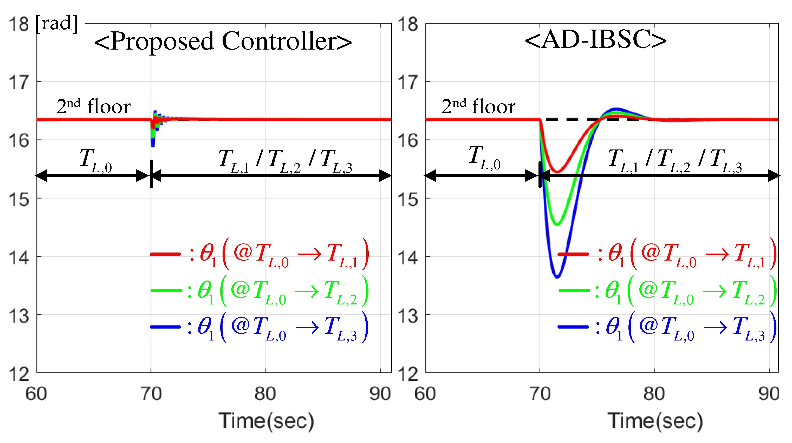
5.3. Case 2: Constant Reference Regulation

This section fixes the floor reference to $p_{ref}=2$nd floor under the settings of $f_{pc}=0.06$ Hz and the no-load condition (no payload for the elevator system). To investigate the floor regulation performance, the light ($T_{L,1}$), medium ($T_{L,2}$), and heavy ($T_{L,3}$) loads were suddenly applied to the passenger cart initialized to the no-load condition ($T_{L,0}$). Figure 8 presents the position regulation results by the two controllers. The improvement of control and estimation mechanisms by the proposed controller effectively reduces not only over/undershoot levels but also transient periods for different load changes. The speed synchronization results shown in Figure 9 indicate the considerable reduction in the transient periods by the proposed controller, which contributes to improving the transient positioning behavior presented in Figure 8.

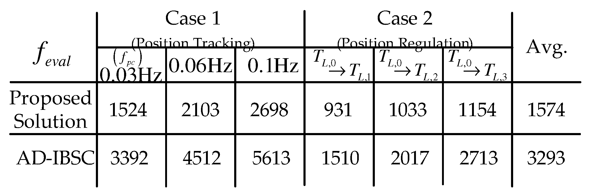
5.4. Numerical Comparison

This section concludes this experimental section by calculating the evaluation function $f_{eval}:=\sqrt{{\int }_0^{\infty }|{\theta }_{ref}\left(t\right)-{\theta }_1{\left(t\right)|}^2+{|{\omega }_1\left(t\right)-{\omega }_2\left(t\right)|}^{2}dt}$ over the experimental data in Section 5.2 and Section 5.3. The table in Figure 10 presents the 52% of performance improvement from the proposed solution in an average manner, which will be significant in practice.

6. Conclusions

The order-reduction technique was applied to devise the model-free speed observer, performance recovery positioning controller, and speed synchronizer, guaranteeing beneficial convergence properties. The closed-loop analysis confirmed to accomplish the control missions under the practical three concerns (marked as (C1), (C2), and (C3) in the introduction section). Finally, a prototype elevator system including the dual BLDCMs as actuators experimentally validated the effectiveness of the proposed controller. The extension to a large power elevator system operated by the three motors will be considered as the future study platform.

References

1. Chen, K.Y.; Huang, M.S.; Fung, R.F. Dynamic modelling and input-energy comparison for the elevator system. Appl. Math. Modell. 2014, 38, 2037–2050. [Google Scholar] [CrossRef]
2. Wang, G.; Qi, J.; Xu, J.; Zhang, X.; Xu, D. Antirollback Control for Gearless Elevator Traction Machines Adopting Offset-Free Model Predictive Control Strategy. IEEE Trans. Ind. Electron. 2015, 62, 6194–6203. [Google Scholar] [CrossRef]
3. Yoo, M.S.; Park, S.W.; Lee, H.J.; Yoon, Y.D. Offline Compensation Method for Current Scaling Gains in AC Motor Drive Systems with Three-Phase Current Sensors. IEEE Trans. Ind. Electron. 2021, 68, 4760–4768. [Google Scholar] [CrossRef]
4. Benosman, M. Lyapunov-Based Control of the Sway Dynamics for Elevator Ropes. IEEE Trans. Control Syst. Technol. 2014, 22, 1855–1863. [Google Scholar] [CrossRef] [Green Version]
5. Pisharam, S.M.; Agarwal, V. Novel High-Efficiency High Voltage Gain Topologies for AC–DC Conversion with Power Factor Correction for Elevator Systems. IEEE Trans. Ind. Appl. 2018, 54, 6234–6246. [Google Scholar] [CrossRef]
6. Benevieri, A.; Carbone, L.; Cosso, S.; Kumar, K.; Marchesoni, M.; Passalacqua, M.; Vaccaro, L. Surface Permanent Magnet Synchronous Motors’ Passive Sensorless Control: A Review. Energies 2022, 15, 7747. [Google Scholar] [CrossRef]
7. Zhang, X.; Wang, Z.; Liu, T. Anti-Disturbance Integrated Position Synchronous Control of a Dual Permanent Magnet Synchronous Motor System. Energies 2022, 15, 6697. [Google Scholar] [CrossRef]
8. Chen, C.S.; Hu, N.T. Model Reference Adaptive Control and Fuzzy Neural Network Synchronous Motion Compensator for Gantry Robots. Energies 2022, 15, 123. [Google Scholar] [CrossRef]
9. Lim, S.; Kim, S.K.; Kim, K.C. Model-Independent Observer-Based Current Sensorless Speed Servo Systems with Adaptive Feedback Gain. Actuators 2022, 11, 126. [Google Scholar] [CrossRef]
10. Sul, S.K. Control of Electric Machine Drive Systems; Wiley-IEEE Press: Hoboken, NJ, USA, 2011. [Google Scholar]
11. Olalla, C.; Leyva, R.; Queinnec, I.; Maksimovic, D. Robust Gain-Scheduled Control of Switched-Mode DC-DC Converters. IEEE Trans. Power Electron. 2012, 27, 3006–3019. [Google Scholar] [CrossRef]
12. Su, J.T.; Liu, C.W. Gain scheduling control scheme for improved transient response of DC-DC converters. IET Power Electron. 2012, 5, 678–692. [Google Scholar] [CrossRef]
13. Liu, X.; Guo, H.; Cheng, X.; Du, J.; Ma, J. A Robust Design of the Model-Free-Adaptive-Control-Based Energy Management for Plug-in Hybrid Electric Vehicle. Energies 2022, 15, 7467. [Google Scholar] [CrossRef]
14. Zuo, S.; Zhang, Y.; Wang, Y. Adaptive Resilient Control of AC Microgrids under Unbounded Actuator Attacks. Energies 2022, 15, 7458. [Google Scholar] [CrossRef]
15. Qu, W.; Chen, G.; Zhang, T. An Adaptive Noise Reduction Approach for Remaining Useful Life Prediction of Lithium-Ion Batteries. Energies 2022, 15, 7422. [Google Scholar] [CrossRef]
16. Kim, S.K.; Lee, J.S.; Lee, K.B. Self-Tuning Adaptive Speed Controller for Permanent Magnet Synchronous Motor. IEEE Trans. Power Electron. 2017, 32, 1493–1506. [Google Scholar] [CrossRef]
17. Kim, S.K. Robust adaptive speed regulator with self-tuning law for surfaced-mounted permanent magnet synchronous motor. Control Eng. Pract. 2017, 61, 55–71. [Google Scholar] [CrossRef]
18. El-Sousy, F.F.M.; Abuhasel, K.A. Nonlinear Robust Optimal Control via Adaptive Dynamic Programming of Permanent-Magnet Linear Synchronous Motor Drive for Uncertain Two-Axis Motion Control System. IEEE Trans. Ind. Appl. 2020, 56, 1940–1952. [Google Scholar] [CrossRef]
19. Kim, S.K.; Kim, Y.; Ahn, C.K. Energy-Shaping Speed Controller with Time-Varying Damping Injection for Permanent-Magnet Synchronous Motors. IEEE Trans. Circuits Syst. II Express Briefs 2021, 68, 381–385. [Google Scholar] [CrossRef]
20. Kim, S.K.; Ahn, C.K. Position Regulator with Variable Cut-Off Frequency Mechanism for Hybrid-Type Stepper Motors. IEEE Trans. Circuits Syst. I Regul. Pap. 2020, 67, 3533–3540. [Google Scholar] [CrossRef]
21. Li, Z.; Zhang, Z.; Wang, J.; Wang, S.; Chen, X.; Sun, H. ADRC Control System of PMLSM Based on Novel Non-Singular Terminal Sliding Mode Observer. Energies 2022, 15, 3720. [Google Scholar] [CrossRef]
22. Zhou, X.; Wang, C.; Ma, Y. Vector Speed Regulation of an Asynchronous Motor Based on Improved First-Order Linear Active Disturbance Rejection Technology. Energies 2020, 13, 2168. [Google Scholar] [CrossRef]
Figure 1. Hardware and software configuration of dual-motor elevator system.
Energies 15 09147 g001
Figure 2. Proposed algorithm with speed synchronizer for output-feedback multi-loop positioning system.
Energies 15 09147 g002
Figure 3. Design factors for the proposed algorithm.
Energies 15 09147 g003
Figure 4. Experimental setup.
Energies 15 09147 g004
Figure 5. Position response comparison (master motor) for different outer loop cut-off frequency.
Energies 15 09147 g005
Figure 6. Speed synchronization error comparison (slave motor) for different outer loop cut-off frequency.
Energies 15 09147 g006
Figure 7. Speed estimation error and DOB.
Energies 15 09147 g007
Figure 8. Position response comparison (master motor) for different load variations.
Energies 15 09147 g008
Figure 9. Speed synchronization error comparison (slave motor) for different load variations.
Energies 15 09147 g009
Figure 10. Numerical comparison result.
Energies 15 09147 g010
Publisher’s Note: MDPI stays neutral with regard to jurisdictional claims in published maps and institutional affiliations.