CFD-DEM Simulation of Particle Fluidization Behavior and Glycerol Gasification in a Supercritical Water Fluidized Bed

Abstract

In this study, a mathematical model of hydrogen production from glycerol gasification in supercritical water was established based on the CFD-DEM method. The fluidization process of a supercritical water fluidized bed and the effects of bed height and feed structure on particle distribution and residence time of feedstock were analyzed. Additionally, the temperature field in the fluidized bed, the reaction rate distribution of each reaction and the influence of wall temperature on gas yields were also studied. The simulation results show that the bubble channel is easy to form along the wall at one side of the feed inlet. When the initial bed height is high, and the double symmetric feed inlet structure is used, the residence time of the feedstock is prolonged. The pyrolysis of glycerol mainly occurs in the middle and lower part of the fluidized bed reactor, and the reaction rate of the water gas shift reaction and methanation reaction are highest near the outlet, and a high wall temperature is conducive to the glycerol gasification.

1. Introduction

The massive use of fossil fuels has caused serious energy and environmental problems. It is urgent to develop renewable energy technologies. As a renewable and green energy, hydrogen is regarded as a good alternative fuel because of its advantages, such as high combustion stability, zero-emission, and high calorific value [1]. Recently, hydrogen production from biomass gasification in supercritical water has attracted more and more attention [2,3,4,5]. Supercritical water refers to water whose temperature and pressure are higher than the critical point (374 °C, 22.1 MPa). Supercritical water is a solvent with low viscosity, high diffusion and low dielectric constant, and good solubility, which are beneficial to improve the reaction rate [6]. To solve the problems of reactor blockage and low gasification efficiency in tubular reactors, Lu et al. [7] successfully developed a fluidized bed reactor for hydrogen production from biomass gasification in supercritical water. However, due to the lack of perfect theories to guide the operation methods and parameters, the current supercritical water fluidized bed still has problems such as uneven temperature distribution, unstable gas products, and bed material outflow [8]. Therefore, it is very important to study the flow and reaction behavior in supercritical water fluidized beds to optimize the reactor parameters, improve the gasification efficiency, and promote the industrial application of fluidized beds.

Due to the extreme conditions of high temperature and high pressure of supercritical water and the lack of measurement method of reaction particle flow, it is difficult to observe the flow details in the fluidized bed reactor with the experiments. With the development of computer technology, numerical simulation has been more and more applied in the study of reactors [9,10,11,12]. At present, the two main methods for simulating fluid dynamics in fluidized beds are the Euler-Euler method and the Euler-Lagrange method.

In the Euler-Euler method, both the fluid phase and the particle phase are considered continuous phases, and the fluid and particle are considered as a continuous medium that exists together and permeates each other. The Euler-Euler method is not only widely used in industrial applications, but also can obtain good calculation results in some complex or fine small-scale geometric simulations. The most important model of the Euler-Euler method is the two-fluid model (TFM), which is usually used in conjunction with the kinetic theory of granular flow (KTGF) to give particles properties like fluids, such as viscosity and pressure. Wei et al. [1] used the TFM-KTGF method in Fluent to simulate the particle distribution and residence time distribution in a supercritical water fluidized bed reactor and studied the influence of different feeding methods and feeding rates on the solid particle distribution. The results show that the structure of the double symmetrical inlet with 45 degrees downward is the best, and the residence time of the inlet is affected by the number of large bubbles and the expansion height of the bed. Su et al. [13] established a comprehensive three-dimensional hydrodynamic numerical model to simulate the process of glucose gasification in a supercritical water fluidized bed reactor and predicted the flow behavior of particles, the distribution of reaction rates, and the distribution of gas products. Yao et al. [14] used the TFM-KTGF method to describe the process of glucose gasification in supercritical water and studied the temperature field in the fluidized bed, the influence of operating conditions and reactor structure on the gas yield and residence time of gas products. Based on the TFM model, Wu et al. [15] designed the velocity partition zones for the slant distributor structure of a supercritical water fluidized bed reactor and improved the predictive correlation of the minimum fluidization velocity proposed by Lu et al. [8].

However, because the Euler-Euler model considers the particle phase as quasi-fluid, the discrete character of the particle phase is lost, and the details of the particle scale cannot be obtained from the numerical simulation. Additionally, TFM is more sensitive to particle kinetic parameters, and some data of TFM depends on the distribution of solid particles in the fluidized bed rather than on the real properties of the particles (static, dynamic, and rotational friction quantity, etc.) [16]. However, the Euler-Lagrange model includes the static, dynamic, and rotating quantities of the particle, which define the main characteristics of the solid particle. The Euler-Lagrange models mainly include Dense Discrete Phase Model (DDPM), Multiphase Particle-in-cell (MP-PIC) Model, and the Discrete Element Method (DEM). DEM can track a specific particle, accurately simulate the interaction force between particles, and fully reflect the discrete properties of particles. Thus, the heat and mass transfer and chemical reaction process in a fluidized bed can be better simulated by using DEM. However, DEM needs more computational resources, so it is more used to simulate fluidized beds with fewer particles.

Lu et al. [17] compared the flow structure and bubble dynamics of supercritical water fluidized bed and gas fluidized bed under different operating conditions based on a DEM, and observed the fluidization transition, particle mixing and kinetic characteristics, and bubble characteristics in the two fluidized beds. By adopting Fluent coupled with EDEM, Zhao et al. [18] simulated the glucose gasification in supercritical water, studied the bed dynamic behavior and chemical reaction kinetics and explored the influence of operation parameters on gas production rate and carbon gasification efficiency. Zhang et al. [19] studied the influence of particle size distributions (PSD) on the minimum fluidization velocity of a supercritical water fluidized bed reactor based on the CFD-DEM method. The results show that the minimum fluidization velocity of Flat-type PSD is the smallest. Mono-type PSD has the highest minimum fluidization velocity. Zhang et al. [20] also studied the effect of the particle aspect ratio of cylindrical particles on the minimum fluidization velocity. The increase of aspect ratio leads to the increase of bed void fraction and finally to the increase of minimum fluidization velocity. Based on the CFD-DEM method, Lu et al. [21,22] proposed a method to deal with the boundary conditions of constant wall flux in a fluidized bed and applied it to a supercritical water fluidized bed reactor. They studied the influence of operating conditions and particle properties on the heat transfer characteristics of the wall bed in a supercritical water fluidized bed. It is verified that this method is more accurate than the Lattanzi method in predicting the heat transfer coefficient of a fluidized bed.

At present, there is little published literature on the exploration of hydrogen production from biomass gasification in supercritical water fluidized bed based on the CFD-DEM method, and no simulation results of CFD-DEM for hydrogen production from glycerol gasification in supercritical water are available. The innovative research contents of this study include:

(1)

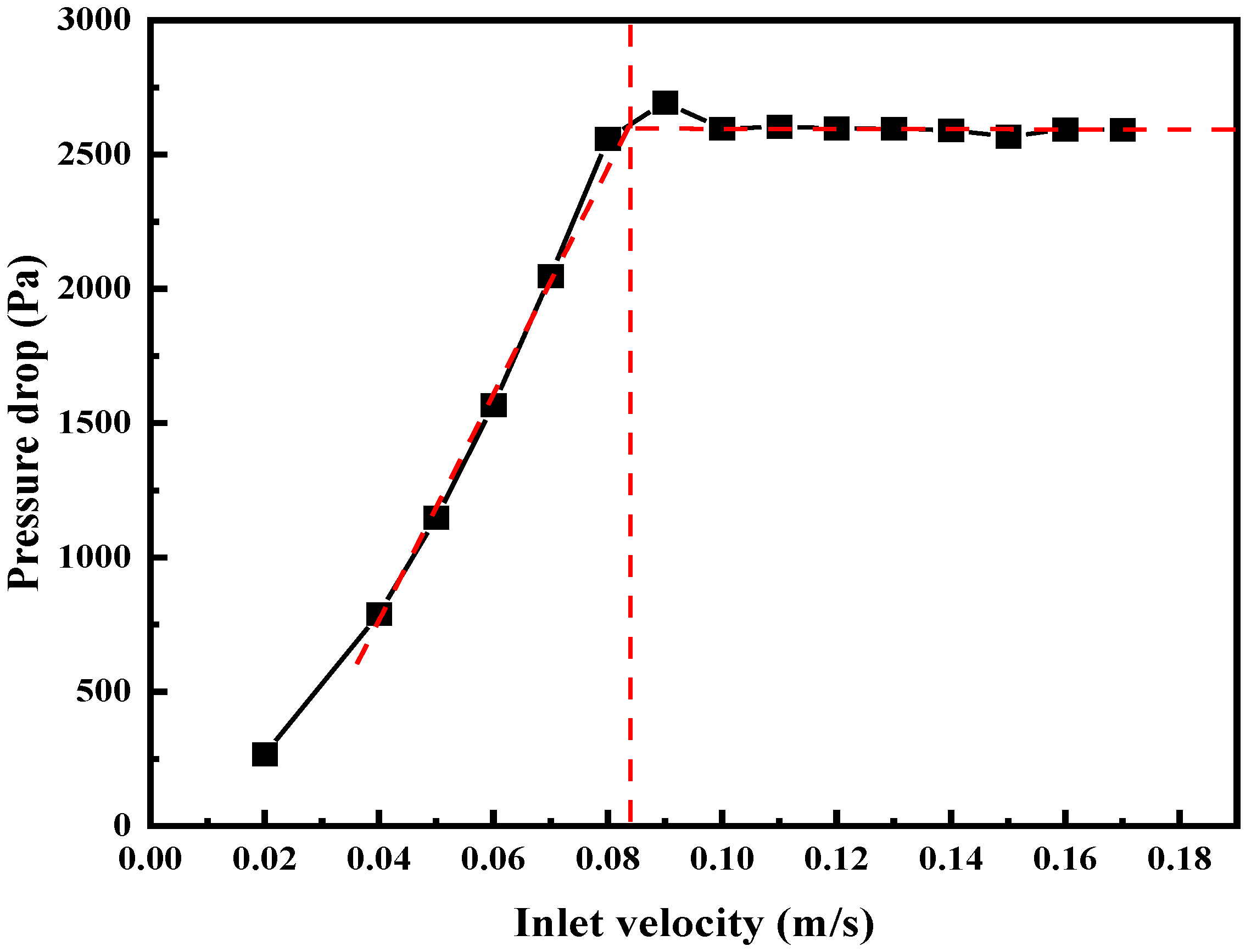
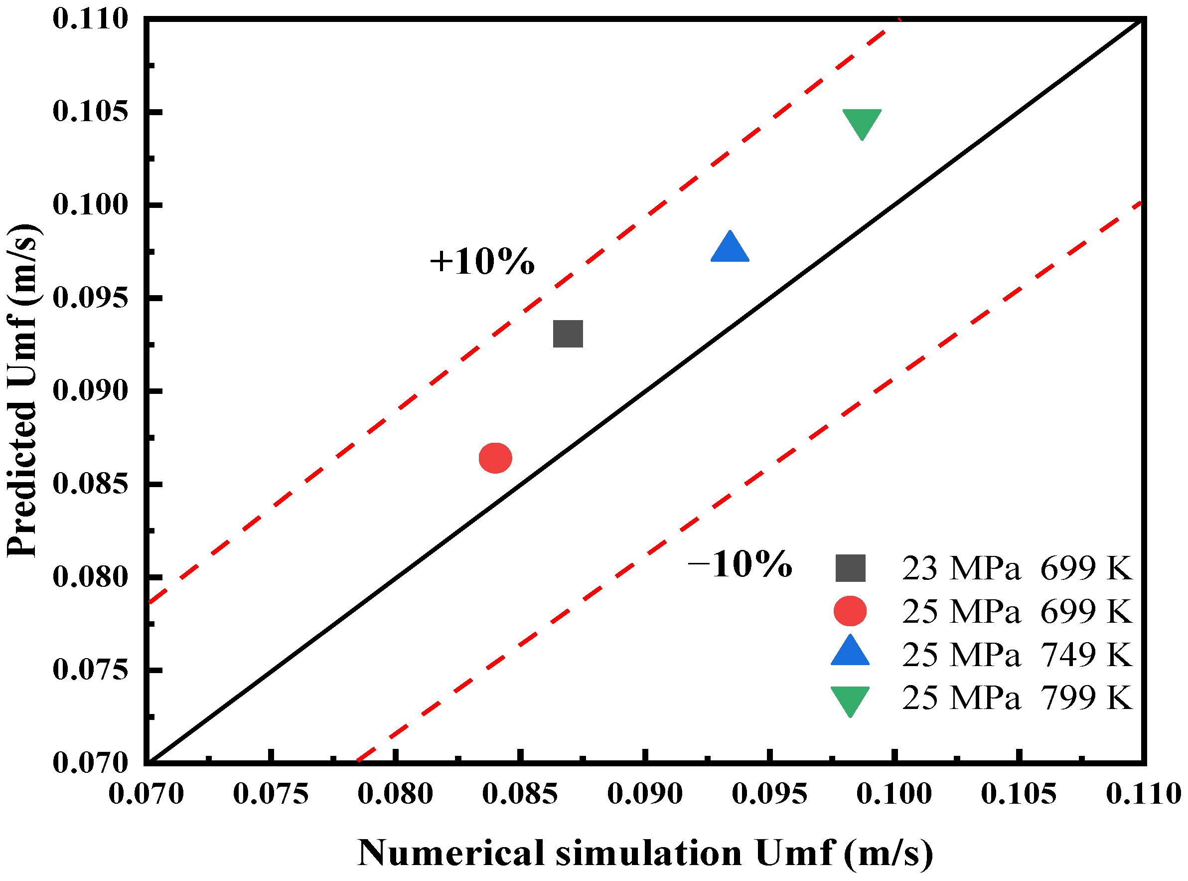
A supercritical water fluidized bed reactor model considering flow, heat transfer, and glycerol gasification reaction was established, and the model was verified by using the predictive correlation of the minimum fluidization velocity of the supercritical water fluidized bed.

(2)

The effect of initial bed height and feeding method on the characteristics of bed particle distribution and residence time distribution in fluidized bed reactor were studied.

(3)

CFD-DEM was coupled with the reaction kinetic model of supercritical water gasification of glycerol to predict the gasification results under different wall temperatures.

2. Model Description

2.1. Fluid Phase

In supercritical water, organic compounds and gases can be completely dissolved. Therefore, the fluid phase can be considered as a homogeneous mixture, which can be described by a set of CFD equations, as follows:

Continuity equation:

$$\frac{\partial }{\partial t}\left({\alpha }_f{\rho }_f\right)+\nabla \cdot \left({\alpha }_f{\rho }_f{\overrightarrow{v}}_f\right)=0,$$

(1)

where ${\alpha }_f$, ${\rho }_f$, ${\overrightarrow{v}}_f$ are the volume fraction, physical density, and velocity of the fluid phase, respectively.

Momentum equation:

$$\frac{\partial }{\partial t}\left({\alpha }_f{\rho }_f{\overrightarrow{v}}_f\right)+\nabla \cdot \left({\alpha }_f{\rho }_f{\overrightarrow{v}}_f{\overrightarrow{v}}_f\right)=-{\alpha }_f\nabla \cdot p+\nabla \left({\alpha }_f{\tau }_f\right)+{\alpha }_f{\rho }_{f}g-K_{fp}\left({\overrightarrow{v}}_f-{\overrightarrow{v}}_p\right),$$

(2)

where $p$ is the pressure, ${\tau }_f$ is the fluid corresponding force tensor, $g$ is the gravitational acceleration, ${\overrightarrow{v}}_p$ is the particle phase velocity, and $K_{fp}$ is the phase momentum exchange coefficient between the particle phase and the fluid phase. The value of $K_{fp}$ comes from the Gidaspow model, which will be described below.

Energy equation:

$$\frac{\partial }{\partial t}\left({\alpha }_f{\rho }_f{H}_f\right)+\nabla \left({\alpha }_f{\rho }_f{\overrightarrow{v}}_f{H}_f\right)=\nabla \left({\lambda }_f\nabla T_f\right)+Q_{pf}+S_q,$$

(3)

where $H_f$ is the specific enthalpy of the fluid phase, $\lambda$ is thermal conductivity, $T$ is temperature, $Q_{pf}$ is the intensity of heat exchange between fluid and particle, and $S_q$ is a source term that includes sources of enthalpy.

Species transport equation:

$$\frac{\partial }{\partial t}\left({\alpha }_f{\rho }_f{Y}_i\right)+\nabla \cdot \left({\alpha }_f{\rho }_f{Y}_i{\overrightarrow{v}}_f\right)=-\nabla \cdot {\alpha }_f{J}_i+{\alpha }_f{R}_i,$$

(4)

where $Y_i$ is the mass fraction of specie $i$, $J_i$ is the diffusion flux of specie $i$, $R_i$ is the net production rate due to fluid phase chemical reactions, and

$$J_i=-{\rho }_f{D}_{i,m}\nabla Y_i,$$

(5)

where $D_{i,m}$ is the diffusion coefficient of the specie $i$ in the mixture.

The heat transfer between fluid and particle is calculated using the Ranz-Marshall model.

$$N{u}_p=2.0+0.6{\mathrm{Re}}_p^{1/2}{\mathrm{Pr}}^{1/3},$$

(6)

$$Q_{fp,j}=h_{fp}\pi d_p^2\left(T_f-T_{p,j}\right),$$

(7)

$$Q_{pf}=-{\displaystyle \sum _{j=1}^n{Q}_{fp,j}/V_{cell}},$$

(8)

$$h_{fp}=\frac{{\lambda }_{f}N{u}_p}{d_p},$$

(9)

where $R{e}_p$ is the relative Reynolds number, $\mathrm{Pr}$ is the Prandtl number, $h_{fp}$ is the heat transfer coefficient between fluid and particle, $j$ represents the particle index, $n$ is the number of particles in a fluid cell, $V_{cell}$ is the volume of a fluid cell.

The expression $R{e}_p$ is calculated as follows

$$R{e}_p=\frac{{\rho }_f{d}_p\left|{\overrightarrow{v}}_p-{\overrightarrow{v}}_f\right|}{{\mu }_f},$$

(10)

2.2. Particle Phase

Each particle in the particle flow has 6 degrees of freedom, including translational and rotational motions. In the DEM method, Newton’s second law is used to solve the translational acceleration and rotational acceleration of each solid particle respectively.

The translational motion equation:

$$m\frac{d{v}_p}{dt}=F_g+F_c+F_{nc},$$

(11)

where $v_p$ is the translational velocity of the particle, $m$ is the mass of the particle, $F_g$ is the resultant gravitational force acting on the particle, $F_c$ and $F_{nc}$ are the resultant contact and noncontact forces between the particle and surrounding particles or walls.

The rotational motion equation:

$$I\frac{d\omega }{dt}=M,$$

(12)

where $I$ is the moment of inertia, $\omega$ is the angular velocity, $M$ is the resultant contact torque acting on the particle, and $t$ is time.

For materials with a small particle size and high thermal conductivity, the internal thermal conductivity of the particles can usually be ignored [23], so the internal heat transfer of the particles is not considered in this paper. The heat flux between particles is defined by [24]

$$Q_{p1p2}=h_c\Delta T_{p1p2},$$

(13)

where $Q_{p1p2}$ and $T_{p1p2}$ are the heat flux and temperature difference between particles one and two, respectively. The contact area is added to the heat transfer coefficient $h_c$, which is expressed as

$$h_c=\frac{4k_{p1}{k}_{p2}}{k_{p_1}+k_{p2}}{\left[\frac{3F_N{r}^{\ast }}{4E^{\ast }}\right]}^{1/3},$$

(14)

where $F_N$ is the normal force, $r^{\ast }$ is the particle geometric mean radius calculated from Hertz elastic contact theory [25], and $E^{\ast }$ is the effective Young’s modulus. The bracketed term on the right side of the equation is used to model the contact area between particles.

The Soft-sphere model [26] was used to calculate the interaction force between particles. In the soft-sphere model, particles are assumed to be rigid, and tiny overlaps are used to represent the deformation during particle contact. The contact force between two spherical particles can be modeled by using a simple system of springs, dashboards, and sliders.

2.3. Interphase Force

The Gidaspow model has been extensively verified by experimental data, and the applicability of the Gidaspow model in supercritical water fluidized beds was also demonstrated by Lu et al. [27,28]. In this study, Gidaspow’s [29] drag model was used to simulate the interaction force between the two phases.

When ${\alpha }_f>0.8$,

$$K_{fp}=\frac{3}{4}{C}_D\frac{{\alpha }_p{\alpha }_f{\rho }_f\left|{\overrightarrow{v}}_p-{\overrightarrow{v}}_f\right|}{d_p}{\alpha }_f^{-265},$$

(15)

When ${\alpha }_f\le 0.8$,

$$K_{fp}=150\frac{{\alpha }_p\left(1-{\alpha }_f\right){\mu }_f}{{\alpha }_f{d}_p^2}+1.75\frac{{\rho }_f{\alpha }_p\left|{\overrightarrow{v}}_p-{\overrightarrow{v}}_f\right|}{d_p},$$

(16)

where ${\alpha }_p$, ${\overrightarrow{v}}_p$ and $d_p$ are the particle volume fraction, velocity, and diameter, respectively, and ${\mu }_f$ is the fluid dynamic viscosity. $C_D$ is the drag coefficient, which is defined by

$$C_D=\frac{24}{{\alpha }_{f}R{e}_p}\left[1+0.15{\left({\alpha }_{f}R{e}_p\right)}^{0.687}\right],$$

(17)

2.4. Chemical Reaction Kinetics Model

A kinetic model of supercritical water gasification of glycerol-based on lumped parameter method proposed by Guo et al. [30] was used in this paper to simplify the whole gasification process into a combination of multiple reactions. Because it is very difficult to take all intermediates into account in chemical reactions, the average molecular formula of the intermediate “Int” in the model of Guo et al. was assumed to be C₂H₄O. The gasification process involves four types of chemical reactions:

(1)

Glycerol pyrolysis.

$$\mathrm{Reaction} 1: {\mathrm{C}}_3{\mathrm{H}}_8{\mathrm{O}}_3 \stackrel{K_1}{⟶}{ \mathrm{Int}+\mathrm{CO}}_2{+2\mathrm{H}}_2$$

(18)

$$\mathrm{Reaction} 2: {\mathrm{C}}_3{\mathrm{H}}_8{\mathrm{O}}_3 \stackrel{K_2}{⟶}{ \mathrm{Int}+\mathrm{CO}+\mathrm{H}}_2{+\mathrm{H}}_2\mathrm{O}$$

(19)

(2)

Intermediates steam reforming.

$$\mathrm{Reaction} 3: {\mathrm{Int}+\mathrm{H}}_2\mathrm{O} \stackrel{K_3}{⟶} 2\mathrm{CO}+3{\mathrm{H}}_2$$

(20)

$$\mathrm{Reaction} 4: {\mathrm{Int}+3\mathrm{H}}_2\mathrm{O} \stackrel{K_4}{⟶}{ 2\mathrm{CO}}_2{+5\mathrm{H}}_2$$

(21)

(3)

Intermediates pyrolysis.

$$\mathrm{Reaction} 5: \mathrm{Int} \stackrel{K_5}{⟶}{ \mathrm{CO}+\mathrm{CH}}_4$$

(22)

(4)

Reaction between gases.

$$\mathrm{Reaction} 6: {\mathrm{CO}+\mathrm{H}}_2\mathrm{O} \stackrel{K_6}{⟶}{ \mathrm{CO}}_2{+\mathrm{H}}_2$$

(23)

$$\mathrm{Reaction} 7: {\mathrm{CO}+3\mathrm{H}}_2 \stackrel{K_7}{⟶}{ \mathrm{CH}}_4{+\mathrm{H}}_2\mathrm{O}$$

(24)

Although the water gas shift reaction and methanation reaction are reversible reactions, the rate constants of the above-mentioned reverse reactions are very small. Thus, the reverse reactions of those two reactions are ignored in the kinetic simulation. The specific rate kinetic parameters of the chemical reaction are shown in

Table 1. Kinetic parameters for supercritical water gasification of glycerol.

Reaction Number	A (s−1)	Ea (kJ·mol−1)	Reaction Rate Expression
Reaction 1	102.60	53.3	K1 = 102.60 exp (−53.3 × 107/RT) [C3H8O3]
Reaction 2	102.76	59.8	K2 = 102.76 exp (−59.8 × 107/RT) [C3H8O3]
Reaction 3	106.63	114.1	K3 = 106.63 exp (−114.1 × 107/RT) [Int][H2O]
Reaction 4	106.15	109.6	K4 = 106.15 exp (−109.6 × 107/RT) [Int][H2O]
Reaction 5	104.13	66.7	K5 = 104.13 exp (−66.7 × 107/RT) [Int]
Reaction 6	102.11	76.5	K6 = 102.11 exp (−76.5 × 107/RT) [CO][H2O]
Reaction 7	104.42	74.3	K7 = 104.42 exp (−74.3 × 107/RT) [CO][H2]

.

2.5. Analysis Method

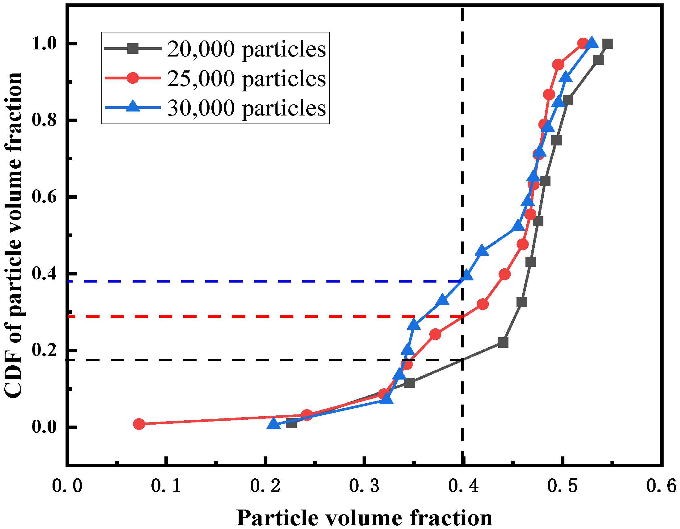
2.5.1. Probability Density Function and Cumulative Distribution Function

The probability density function (PDF) is a function that describes the probability of a random variable near a certain value, which is nonnegative and has the integral of 1 over the whole range of values. The cumulative distribution function (CDF) is the integral of the probability density function, which can completely describe the probability distribution of a random variable. For discrete variables, CDF represents the sum of the occurrence probabilities of all values less than or equal to a certain value. In this paper, the PDF and CDF of the time-averaged particle volume fraction at each location are used to characterize the expansion degree of the bed particles and the area of the channel zone.

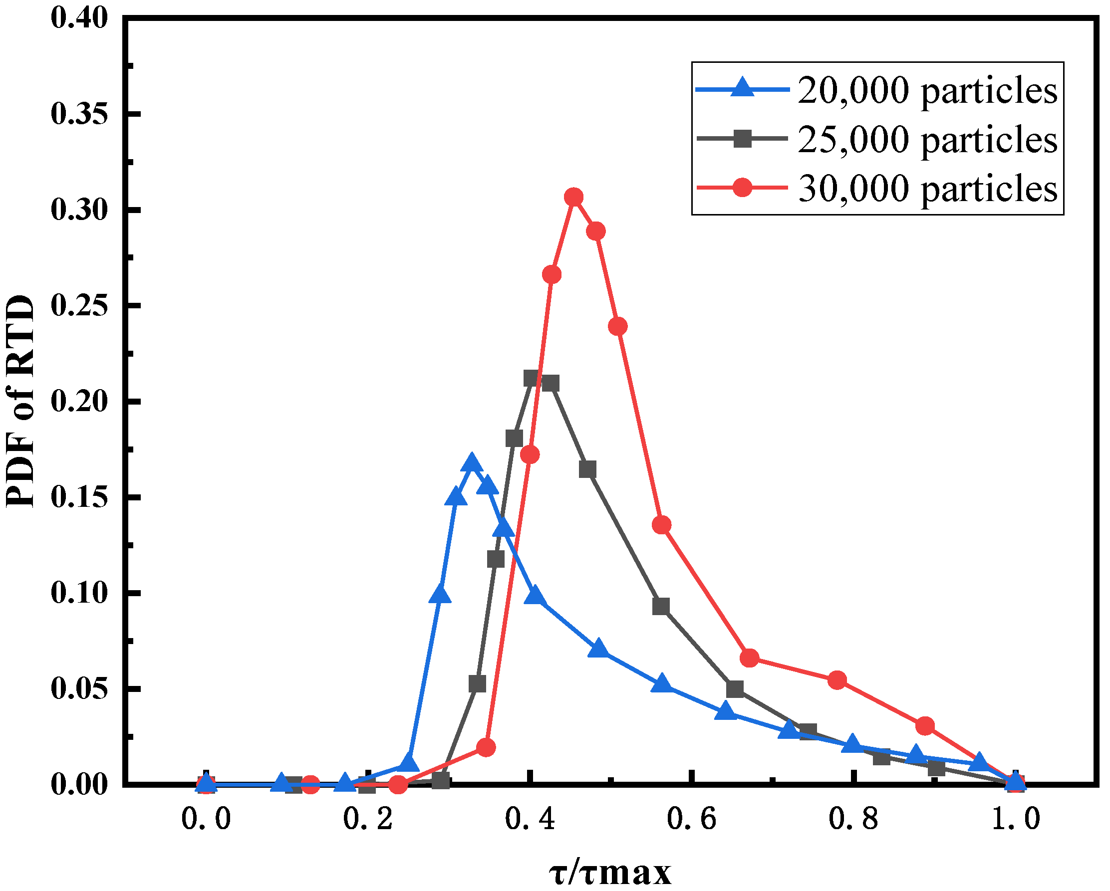
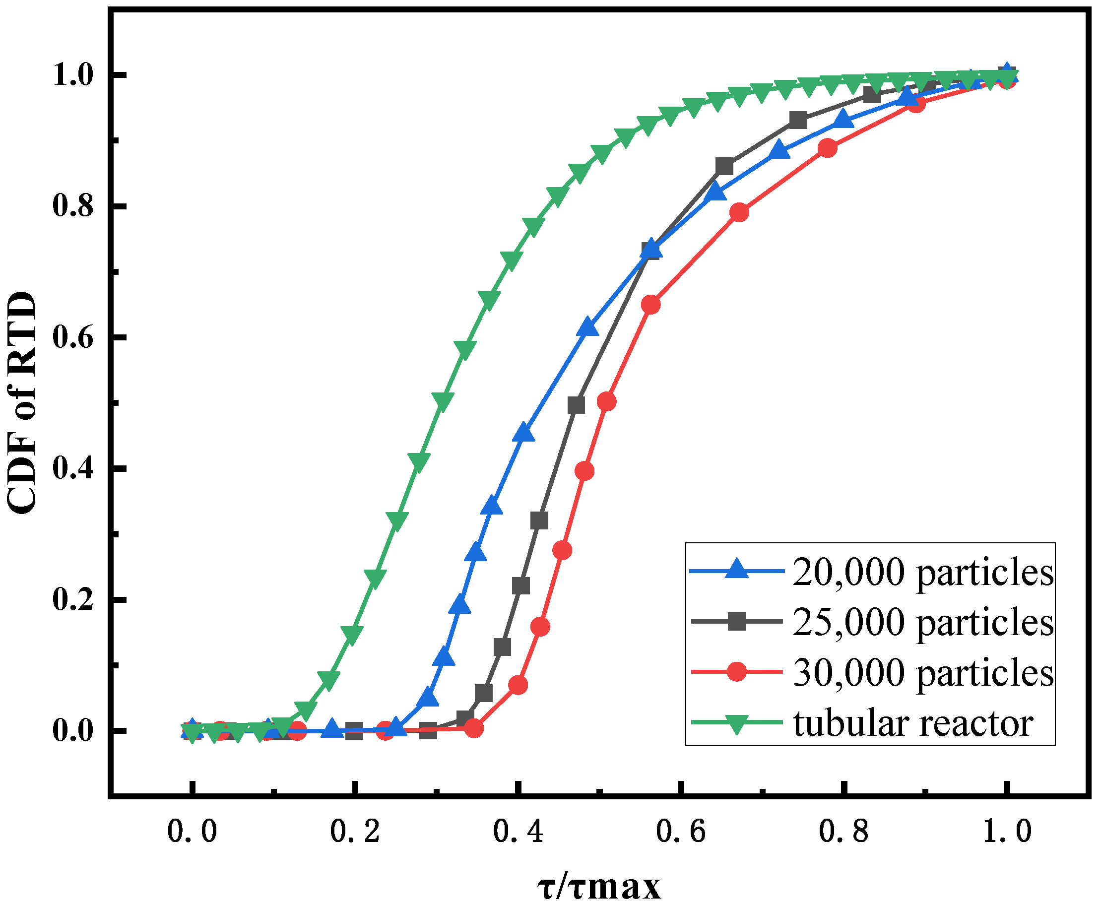
2.5.2. Residence Time Distribution

Residence time refers to the time taken by the feedstock from the inlet to the outlet of a fluidized bed. Residence time distribution (RTD) is an important parameter in the design and operation of a fluidized bed reactor. The method of obtaining residence time distribution by CFD simulation is similar to the experimental tracer technique. When the pressure drop between the inlet and outlet of the bed and the flow rate is stable, a certain amount of tracer whose physical properties are the same as that of the feedstock is added into the fluidized bed. Then, the residence time distribution function $E(t)$ can be calculated by monitoring the variation of tracer concentration $c(t)$ at the outlet of the bed with the fluidization time:

$$E(t)=\frac{c(t)}{{\displaystyle \underset{0}{\overset{\infty }{\int }}c(t)dt}}\approx \frac{c(t_i)}{{\displaystyle \sum _{i=0}^{\infty }c(t_i)\Delta t_i}},$$

(25)

where $c(t)$ is the concentration of the tracer at the time of $t$.

The distribution function of cumulative residence time is the proportion of the feedstock with residence time less than $t$ in the fluidized bed, which is defined as:

$$F(t)={\displaystyle \underset{0}{\overset{t}{\int }}E(t)dt},$$

(26)

${\tau }_{50}$ is used to characterize the residence time of particles, which is defined as follows:

$${\tau }_{50}=\frac{t_{50}}{t_{\max }},$$

(27)

where $t_{50}$ is the time when 50% of the tracer is collected at the outlet, and $t_{\max }$ is the time when all tracers are collected.

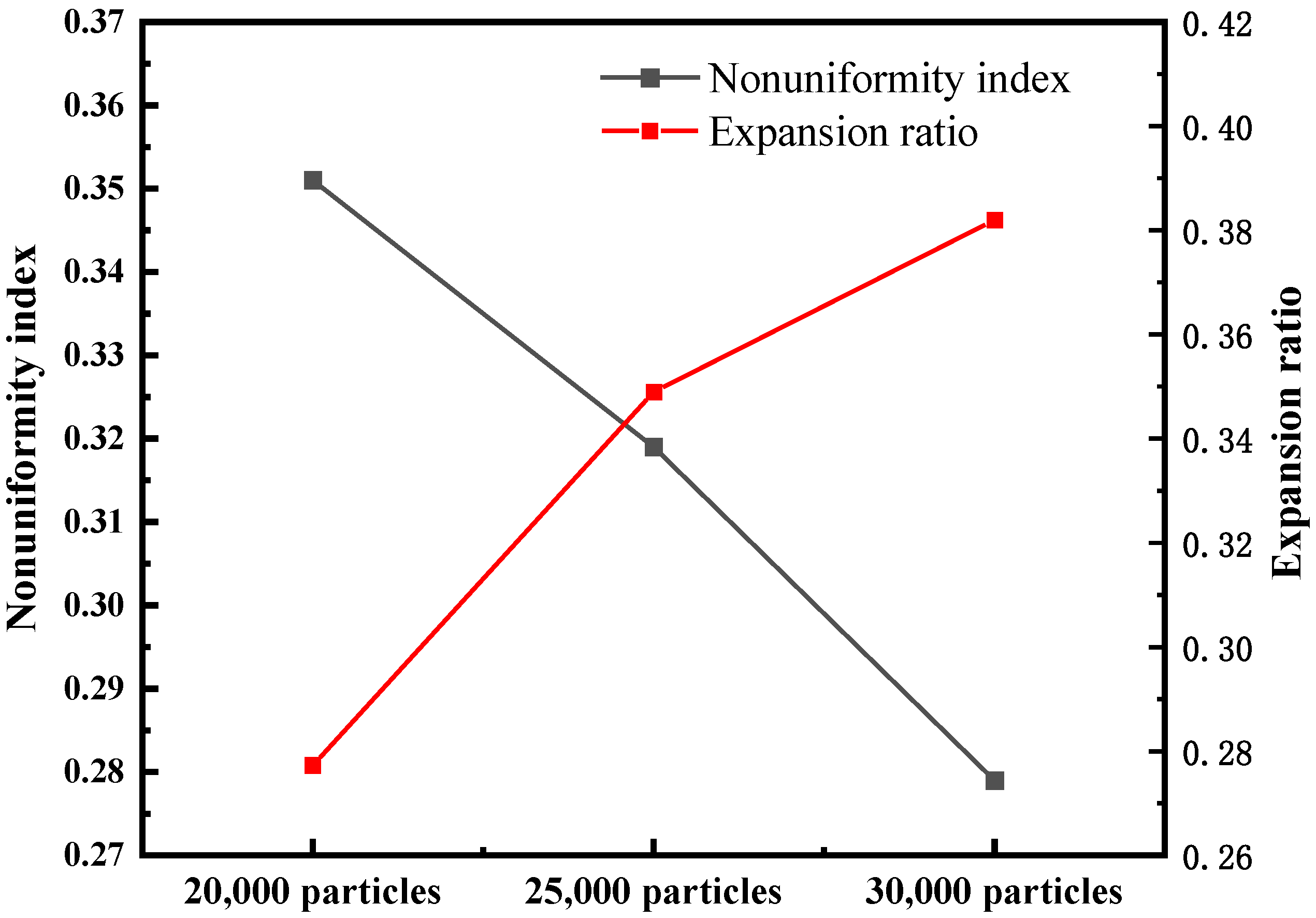
2.5.3. Nonuniformity Index

To quantify the degree of inhomogeneity of the flow field, an inhomogeneity index (NI) is introduced, which is defined as follows [31,32]:

$$NI=\frac{\sqrt{\frac{1}{n-1}{\displaystyle \sum _{i=1}^n{\left({\epsilon }_{p,i}-{\overline{\epsilon }}_p\right)}^2}}}{\sqrt{{\overline{\epsilon }}_p\left({\epsilon }_{p,mf}-{\overline{\epsilon }}_p\right)}},$$

(28)

where the numerator is the particle volume fraction standard deviation and the denominator is the maximum possible value for the particle volume fraction standard deviation. ${\epsilon }_{p,i}$ is the average value of the particle volume fraction in the ith specific ring region, ${\overline{\epsilon }}_p$ is the average particle volume fraction over the whole domain, ${\epsilon }_{p,mf}$ stands for the particle volume fraction at minimum fluidization condition.

2.5.4. Expansion Ratio

$$\mathrm{Expansion} \mathrm{ratio}=\frac{H-H_S}{H_S},$$

(29)

where $H$ is expanded bed height, $H_S$ is the initial static bed height [33].

2.5.5. Gas Yield

Gas yield is used to evaluate gasification characteristics and is calculated as follows [6]:

$$\mathrm{Gas}\text{-}\mathrm{yield}=\frac{\mathrm{molar} \mathrm{amount} \mathrm{of} \mathrm{a} \mathrm{certain} \mathrm{component} \mathrm{of} \mathrm{the} \mathrm{gaseous} \mathrm{products}}{\mathrm{quality} \mathrm{of} \mathrm{glycerin}},$$

(30)

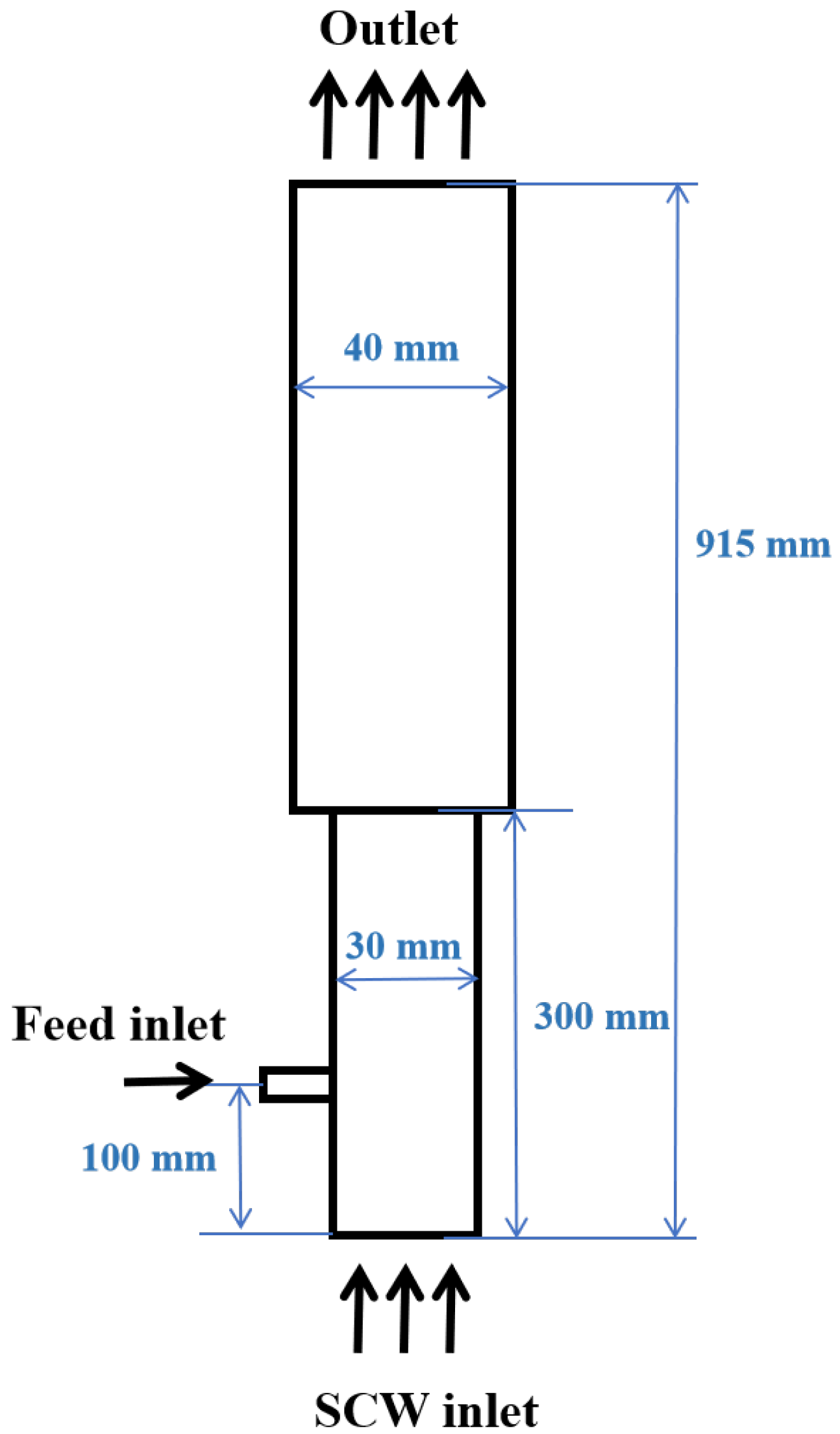
3. Numerical Method and Model Validation

In this paper, the coupling method of CFD and DEM was adopted for numerical simulation. A fluidized bed reactor with a height of 915 mm and a thickness of 5 mm was studied. The width of the fluidized section and expanded section is 30 mm and 40 mm, respectively. The specific size and shape are shown in Figure 1. A uniform grid of 2.5 mm (W) × 2.5 mm (T) × 3 mm (H) was used in the calculation domain. The particles used in the simulation are inert particles with a diameter of 1 mm and a density of 2650 kg/m³. All entries were set as velocity entry, and the exit of the fluidized bed was set as outflow. IAPWS-IF97 [34] was used to calculate the physical properties of water, the RK equation of state [35] was used to estimate the density and specific heat of gases, and the method proposed by Chung et al. [36] was used to calculate the viscosity and thermal conductivity of gas products. The method proposed by He [37] was used to calculate the diffusivity of gases in supercritical water. The density of the mixture was calculated by the volume-weighted mixing law, and the viscosity, specific heat, and thermal conductivity of the mixture were calculated by the mass-weighted mixing law. The specific simulation parameters used in the simulation are shown in

Table 2. Computational conditions and model parameters.

Term	Parameter	Value
Particle phase	Particle shape	Spherical
	Particle density	2650 kg/m3
	Particle diameter	1 mm
	Number of particles	20,000/25,000/30,000
	Poisson‘s ratio	0.25
	Coefficient of Restitution	0.9
	Coefficient of Static Friction	0.15
	Coefficient of Rolling Friction	1 × 10−5
	Heat capacity	630 J/kg·K
	Thermal conductivity	10 W/m2·K
Fluid phase	Pressure	25 MPa
	Temperature at the feed inlet	699 K
	Temperature at the SCW inlet	300 K
	Velocity at the feed inlet	0.0262 m/s
	Velocity at the SCW inlet	0.12 m/s
	Concentration of feed (wt%)	1
Operating condition	Solid phase time step	8 × 10−6 s
	Fluid phase time step	8 × 10−4 s
	Grid size	2.5 mm × 2.5 mm × 3 mm

.

The minimum fluidization velocity is an important parameter in the design and operation of the fluidized bed. The minimum fluidization velocity can be obtained by plotting the apparent velocity against the bed pressure drop. When the apparent velocity is less than the minimum fluidization velocity, the bed pressure drop of the fluidized bed increases with increasing the apparent velocity. However, when the apparent velocity is greater than the minimum fluidization velocity, the bed pressure drop of the fluidized bed is basically unchanged and equal to the effective bed weight of the fluidized bed. In this study, the initial value of inlet velocity was 0.02 m/s. The velocity increments are spaced at 0.01 m/s intervals, while each velocity step is held constant for 1 s. Lu et al. [2] and Zhang et al. [19] have both used this method and demonstrated its feasibility. As shown in Figure 2, the apparent velocity corresponding to the turning point of pressure drop is the minimum fluidization velocity of the fluidized bed.

In this paper, the minimum fluidization velocity calculated by simulation was compared with the minimum fluidization velocity predicted by the correlation proposed by Lu et al. [8] to verify the accuracy of CFD-DEM simulation. The minimum fluidization velocity under four conditions was calculated by the simulation. The density and viscosity of fluid under different conditions are shown in

Table 3. Physical properties of SCW under different pressure and temperature conditions.

Condition	Density	Viscosity
23 MPa 699 K	108.49 kg/m3	2.79 × 10−5 Pa·s
25 Mpa 699 K	125.87 kg/m3	2.86 × 10−5 Pa·s
25 MPa 749 K	97.42 kg/m3	3.00 × 10−5 Pa·s
25 MPa 799 K	83.32 kg/m3	3.18 × 10−5 Pa·s

. Figure 3 shows the comparison between the numerical simulation of the minimum fluidization velocity and the prediction results from the relationship proposed by Lu [8]. It shows that the simulation results are in good agreement with the predicted results under different conditions. The calculation errors are all within 10%, which meets the accuracy requirements of the model.

4. Result and Discussion

4.1. Based Case

Figure 4 shows a snapshot of the particles during fluidization build-up. After the supercritical water starts to flow steadily from the inlet at the bottom of the fluidized bed, when the supercritical water reaches a certain fluid resistance, the particles in the bed begin to loosen. At the beginning of the bed expansion, the particles in the fluidized bed can be observed to rise uniformly as a whole. After that, under the entrainment of small bubbles, the particles rise and float under the action of supercritical water buoyancy. When reaching the upper interface of the bed, the bubbles break, the particles sink by gravity and are carried by the bubbles again, and the cycle goes back and forth. The particles move upward as a whole, and the height of the bed expands stably with time until the dynamic stability is basically maintained, and the fluidization is successfully established. During this process, bubbles form, rise, grow, merge and collapse. The bubbles are formed in the near-wall area at the bottom of the bed, move up to the central area gradually with the flow of supercritical water, and finally merge at a certain height of the bed.

From the instantaneous particle velocity vector diagram shown in Figure 5, two different hydrodynamic behaviors can be observed: the formation of vortices and gulf streams. In the trend of particle flow in the whole bed, different degrees of vortices are formed from the bottom to the top of the bed, which drive the exchange of particles at the center and the near-wall of different bed heights. Different from the randomness of the position of the gulf stream in the fluidized bed without the feed pipe [38], in the model presented in this paper, the gulf stream is formed near the wall on the side without the feed pipe. This is because the resistance near the wall is small, and the particles will have a downward trend. As shown in Figure 5a, near the wall of the side of the feed pipe, the inflow fluid tends to flow upward, so the particles must flow back from top to bottom through the wall of the other side, thus forming a gulf stream in the middle and lower sections of the fluidized bed. The bubbles generated by the feed pipe gradually tend to move to the center. In part b of the fluidized bed, the bubbles rise from the center, so the particles move downward on both sides of the wall in this section. Figure 5c shows the phenomenon of particles falling along the wall after the bubble collapse at the top of the bed.

For better expression, we refer to the upper part of the fluidized bed feed pipe as the upper zone of the fluidized bed and the lower part as the lower zone of the fluidized bed. We find that large bubbles are more likely to appear in the upper zone, which is a big feature different from the fluidized bed without a feed pipe. Because of this bubble characteristic, the volume fraction of particles in the upper and lower zones are different. Figure 6 shows the radial distribution of the time-averaged solid fraction at different bed heights in the fluidized bed. It is easy to see that the particle volume fraction in the lower zone of the fluidized bed is relatively uniform, while the upper zone tends to be inhomogeneous with a lower particle volume fraction in the middle and a higher particle volume fraction on both sides because the bubbles tend to merge in the center. It shows that the feed pipe has a great influence on the particle flow in the upper zone, but a small influence on the lower zone. Due to the inflow of the fluid at the feed pipe, the bubble channel is easily formed near the wall at the height of 100 mm, resulting in insufficient mixing and a small volume fraction of solids.

4.2. The Influence of Initial Bed Height

In this part, the influence of initial bed height on the flow behavior of the fluidized bed is discussed. In this section, fluidized beds with initial particle numbers of 20,000, 25,000, and 30,000 are selected for comparative study. Figure 7 shows the PDF distribution of solid volume fractions for different initial bed heights. The results show that with the increase of bed height, the solid volume fraction corresponding to the peak value of the curve is basically the same, but the peak value of the curve decreases, indicating that in this reactor structure, with the decrease of particle number, the particle distribution is more concentrated.

According to previous work [1,15], the channel zone is defined as the part with a particle volume fraction less than 0.4, so the CDF value corresponding to the particle volume fraction of 0.4 can represent the proportion of the channel zone. In the channel zone, since the contact area between the fluid and the particles is greatly reduced, the mixing degree of the two phases is reduced, and the residence time of the feed in the bed will be shortened. It can be seen from Figure 8 that the area of the channel zone increases with the increase of bed height, which is different from the fluidized bed without the feed pipe structure. The formation of the channel zone is closely related to the easy formation of bubbles at the inlet of the feed pipe. The inlet of the feed pipe continuously generates small bubbles, which move upward and merge to form a channel. It is precise because the fluid flow in the feed pipe has a great influence on the upper zone of the fluidized bed, and the higher the bed height, the larger the proportion of the upper zone. Therefore, the larger the number of particles, the larger the proportion of the channel zone.

Figure 9 shows the PDF of the feed RTD for different initial bed heights. It can be observed that with the increase of the initial bed height, the peak value of PDF increases, and the residence time corresponding to the peak value also increases. The residence time ${\tau }_{50}$ corresponding to the CDF value of 0.5 is used to characterize the relative residence time. The smaller the value of ${\tau }_{50}$, the larger the conveying feed, depending on the bed height, and the shorter the residence time.

In Figure 10, the RTD of the supercritical water fluidized bed is compared with the RTD experimental data of a tubular stirred reactor [39]. The residence time of the fluidized bed is longer than that of the tubular stirred reactor, which is more conducive to the full reaction of reactants. Figure 10 also shows the CDF of the feed RTD for different initial bed heights. The results show that the relative residence time of the 20,000 particles bed is the shortest, and that of the 30,000 particles bed is the longest. However, Figure 9 shows that the channel zone area is the largest for the 30,000-particle bed. This may be the result of a combination of factors. The two key factors that determine residence time are bed expansion height and channel area. On the one hand, as shown in Figure 11, a higher initial bed height corresponds to a larger bed expansion ratio and longer feed residence time. On the other hand, in the case of high initial bed height, the channel zone is larger, which leads to the shortening of residence time. The results after synthesizing multiple factors are as follows: the higher the initial bed height, the longer the residence time of feed. Figure 11 shows the magnitude of the global nonuniformity index (NI) of fluidized beds for three initial bed heights. The smaller the NI, the more uniform the flow field in the fluidized bed. The results show that the greater the initial bed height, the greater the uniformity of the flow field in the supercritical water fluidized bed.

4.3. The Influence of Feeding Structure

In this section, the influence of three different feeding structures on the flow characteristics of the fluidized bed is discussed, respectively, single inlet feeding structure (Type A), symmetric double inlet feeding structure (Type B), and single side double inlet feeding structure (Type C). The structure of three different feeding methods is shown in Figure 12. It should be noted that the total flow rate of the three structures is consistent in the simulation.

Figure 13 shows the instantaneous velocity vector at the inlet of different feed structures. The results show that the fluid at the inlet tends to move upward along the wall. Compared with other types, the type B symmetrical double inlet feeding structure can inhibit the formation of large bubbles by forming more and smaller vortices. The type C feeding structure forms a gulf stream on the side of the non-feeding pipe, which is consistent with the type A feeding mode discussed in Section 4.1. Moreover, the area of the gulf stream formed by the type C feeding structure is larger due to the double inlet on one side.

Figure 14 shows the PDF of the solid volume fraction of different feeding structures. It shows that the particle volume fractions corresponding to the peaks of the PDF curves of the three feeding structures are basically the same. Compared with type A, type B and type C feeding structures have more concentrated particle distribution. Figure 15 shows the CDF of solid volume fraction of different feeding structures. As can be seen, when the particle volume fraction is 0.4, the CDF value corresponding to type A feeding structure is larger, indicating that the channel area in the fluidized bed of type A structure is larger. This is because there are more large bubbles in the type A fluidized bed, and the vortex is larger.

Figure 16 shows the NI of a fluidized bed of different feeding structures. The results show that the NI of the type A feeding structure is the highest and that of the type C feeding structure is the lowest. Compared with the type A feeding structure, the type B structure of the fluidized bed has better uniformity due to the interaction of two convection currents, which inhibits the formation of some large bubbles. As discussed in Section 4.1, the feed pipe fluid has a large effect on the upper zone of the fluidized bed, but a small effect on the lower zone. The type C feeding structure can improve the distribution of the feed in the axial direction, so that the influence area of the feed pipe fluid is enlarged, thereby improving the uniformity of the entire bed.

Figure 17 shows the CDF of the feed RTD of different feeding structures. The results show that the relative residence time of the type B structure is the longest, and the relative residence time of the type C structure is the shortest. This is because the symmetric double inlet feeding structure of type B can suppress the formation of large bubbles through convective interaction, which is beneficial to prolong the residence time of the feed. Although the Type C structure makes the bed material more uniform by improving the axial distribution of the feed, the design of the axial high and low inlets significantly reduces the distance between the high inlet and the outlet, making a portion of the feed flow out of the outlet more quickly, which may be the reason for the final smaller ${\tau }_{50}$.

4.4. Chemical Reaction

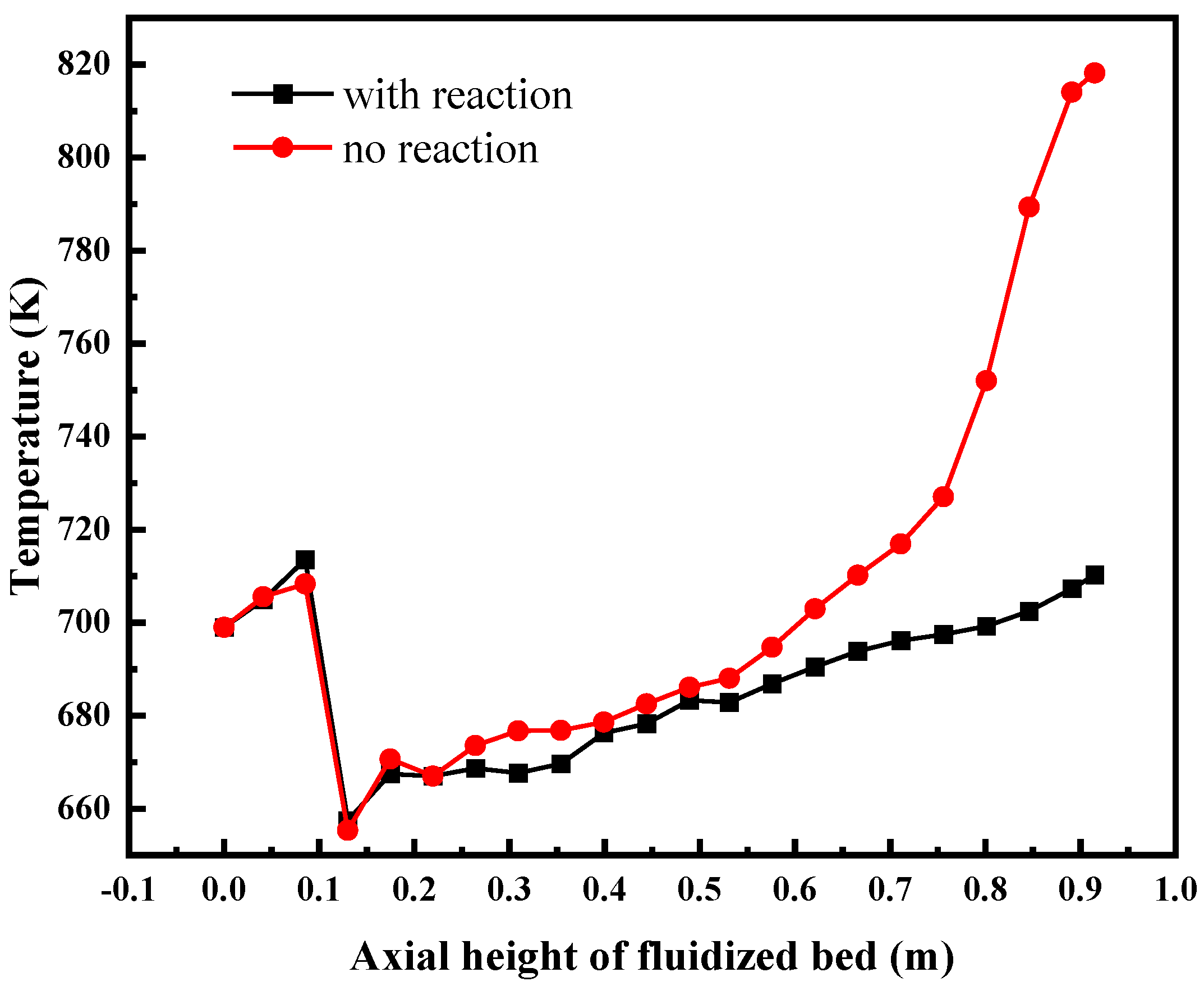
4.4.1. Typical Reaction Case Analysis

To verify the validity of the model, the simulation results of gas products generated by gasification reaction of 300 K 1% low concentration glycerol with 699 K supercritical water under the pressure of 25 MPa were compared with the experimental results of Guo et al. [30]. Among them, the thermal boundary condition is 873 K isothermal condition, the mass flow rate of the supercritical water is 0.00321 kg/s, and the flow ratio of the supercritical water inlet to feed inlet is 4:1. The results show that the simulated value of the outlet temperature is slightly lower than the experimental data, with an error of 8.7%. However, considering that the mass flow rate set in the simulation is 3 times that of the experimental conditions, the reaction will be more violent, the total heat absorbed by the reaction will increase, and the residence time of the fluid in the reactor will be significantly shortened. Moreover, Since the height of the fluidized bed in this paper is 3/4 of the height of the reactor under experimental conditions, the heating time of the fluid is also shortened, so we believe that the error is acceptable. Considering the differences in the reactor model and operating parameters, the chemical kinetic model was also verified by comparing the proportions of each component of the gas products at the reactor outlet gas products. Figure 18 shows that the simulation results are basically consistent with the experimental results, indicating that the model in this paper can accurately describe the gasification reaction process of glycerol in supercritical water. In addition, the value of the Biot number of heat transfer between fluid and solid particles is 0.22, far less than 1, which proves that the temperature distribution inside particles is uniform, so it is reasonable to ignore the heat transfer inside particles in this simulation.

Figure 19 shows the temperature distribution along the central axis of the fluidized bed. The results show that the supercritical water flowing from the bottom inlet is first heated by the wall, and then mixed with the low-temperature feed around the inlet, forming a low-temperature region, and finally continues to be slowly heated by the wall surface as it flows to the outlet. It can be seen from Figure 19 that the temperature of the bed with reaction is lower than that without reaction, indicating that the total thermal effect of all reactions in the whole bed is endothermic.

Figure 20 shows the reaction rate distribution of each chemical reaction along the axis of the fluidized bed. The results show that the pyrolysis reaction of glycerol mainly occurs in the middle and lower part of the reactor due to the influence of the concentration. And in the direction of fluid flow, the pyrolysis reaction rate decreases gradually with the decrease of glycerol concentration. The consumption reaction rate of the intermediate increases with the increase of the height of the fluidized bed and the highest reaction rate is found at the outlet. This may be due to the insufficient reaction of the intermediate. The height of the fluidized bed can be appropriately increased to promote the full reaction of the intermediate and increase the gas production rate. The water gas shift reaction increases with the height of the fluidized bed, which is affected by the concentration of reactants and high temperature. The reaction rate of the methanation reaction is highest at the outlet, which is also due to the high concentration of reactants there.

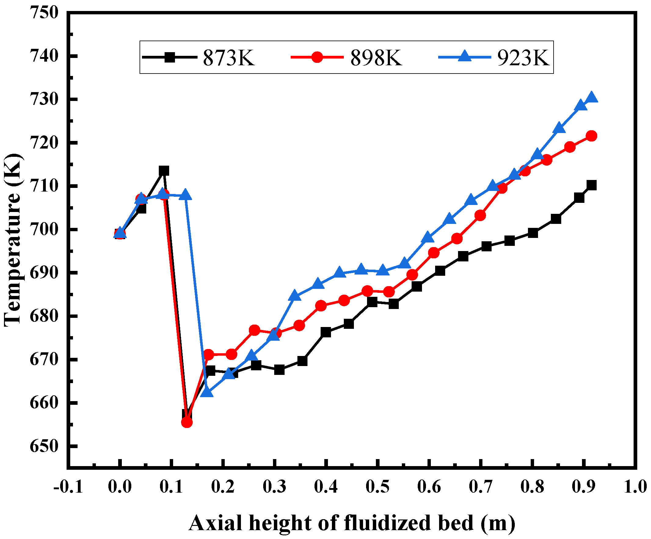
4.4.2. Influence of Wall Temperature

As a typical characteristic parameter of a chemical reaction, temperature plays an important role in the process and result of a chemical reaction. The heat sources inside the fluidized bed include the heat from each inlet material itself, the heat released during the reaction process, and the heat provided by the wall of the fluidized bed. In this section, the influence of wall temperature on the temperature field and the composition of gas products is studied by setting different wall temperatures in fluidized beds.

Figure 21 shows the distribution of the temperature field inside the bed when the wall temperature of the fluidized bed is 873 K, 898 K, and 923 K, respectively. The bulk temperature inside the bed increases as the wall temperature increases. Figure 22 shows the outlet gas product composition at different wall temperatures of the fluidized bed. The results show that with the increase of the wall temperature, the overall temperature inside the bed rises, the chemical reaction rate increases with the increase of the overall temperature in the fluidized bed, and the yield of each gas product increases. According to the simulation results, the higher the bed wall temperature, the better, but in actual production, issues such as catalyst activity and bed heat distribution uniformity need to be considered.

5. Conclusions

Based on the CFD-DEM method, a mathematical model of glycerol gasification in a supercritical water fluidized bed coupled with flow, heat transfer, and gasification reactions was established in this paper. Firstly, the minimum fluidization velocity was compared with the experimental results to verify the reliability of the fluidized bed model. Then, the fluidization process and the distribution of particle velocity field in the fluidized bed were studied, and the effects of bed height and feed structure on the particle distribution and feed residence time were discussed. Finally, the gasification process of glycerol in supercritical water was simulated. The distribution of temperature field and reaction rate in the fluidized bed was discussed, and the composition of gas products in the fluidized bed at different wall temperatures was studied. The conclusions can be summarized as follows:

(1)

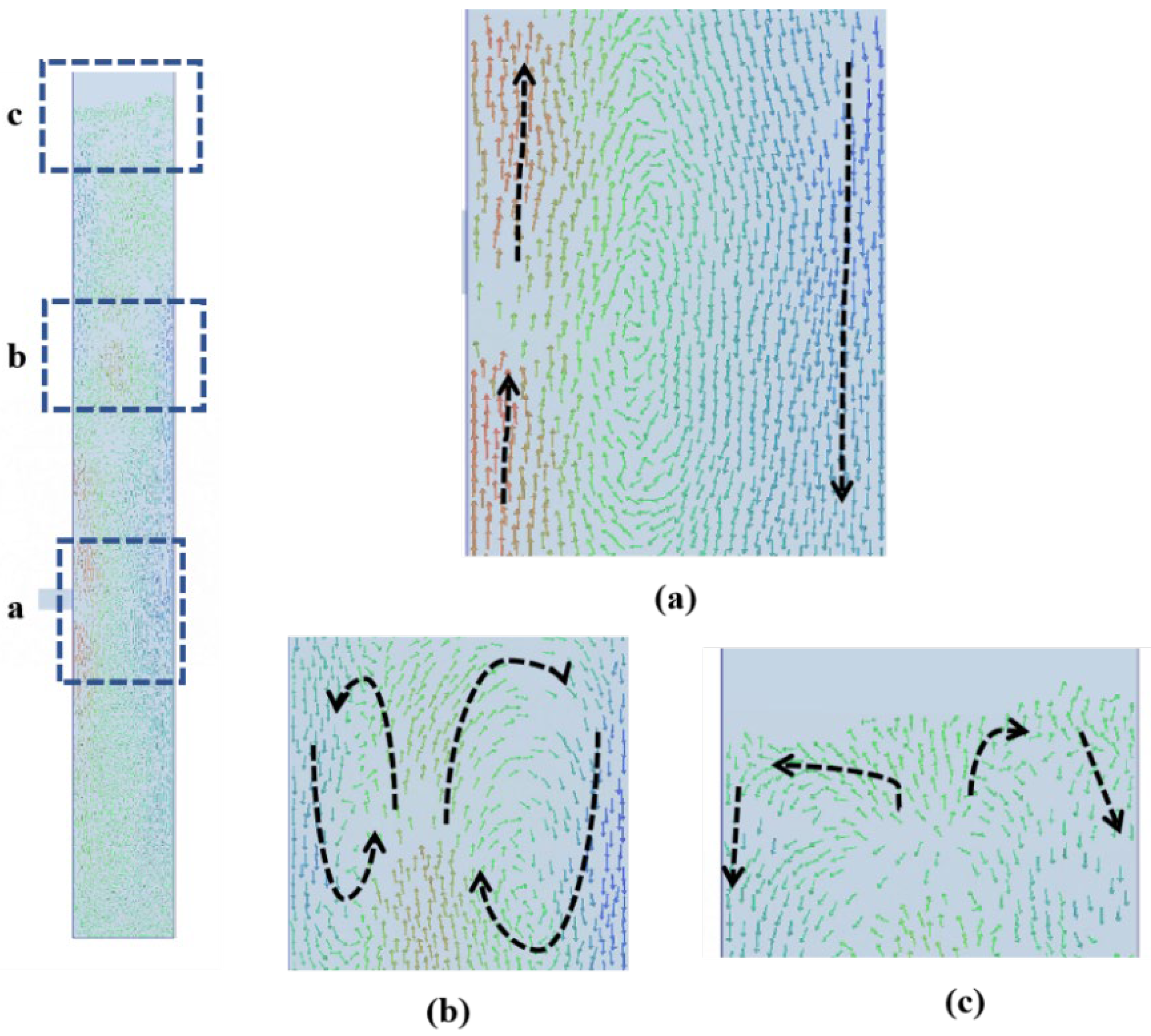
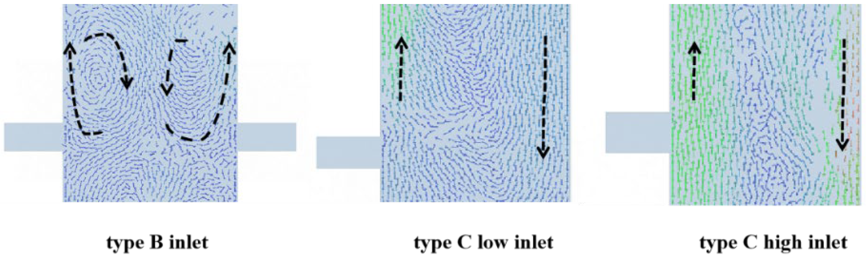
The feed pipe of the fluidized bed has a greater influence on the particle flow in the upper zone but has less influence on the lower zone. The bubble channel is easy to form on the feed pipe side of the fluidized bed, and the gulf stream is easy to form on the side without the feed pipe.

(2)

The higher the initial bed height of the fluidized bed, the more uniform the internal flow field, and the longer the residence time of the feedstock in the fluidized bed.

(3)

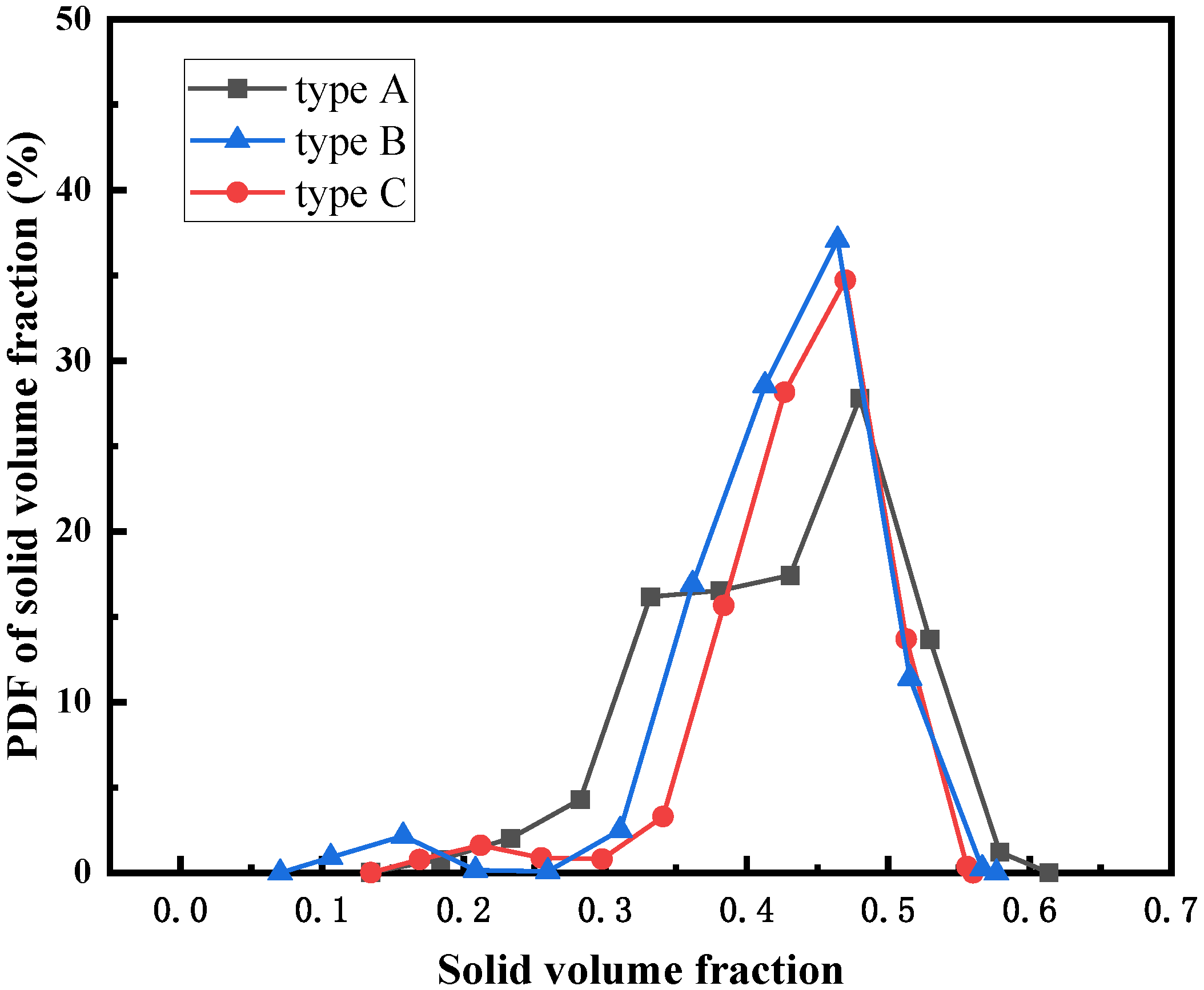
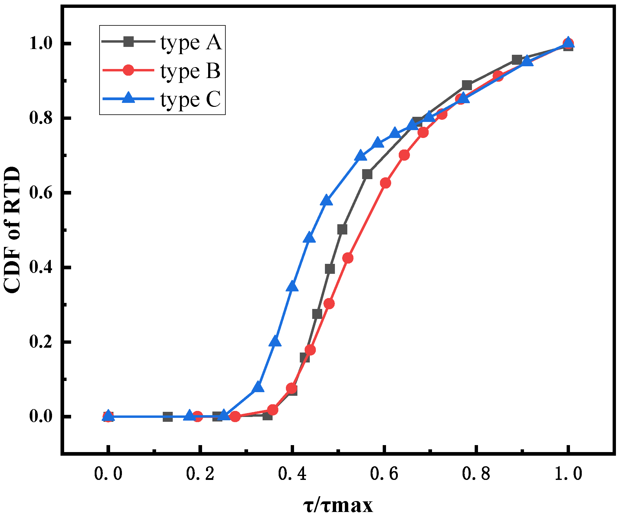
The residence time of the fluidized bed with the symmetric double inlet structure is longer because the convective interaction can inhibit the formation of large bubbles. However, the fluidized bed with a single-side, double inlet, feeding structure shows better uniformity due to the improved feed distribution in the axial direction.

(4)

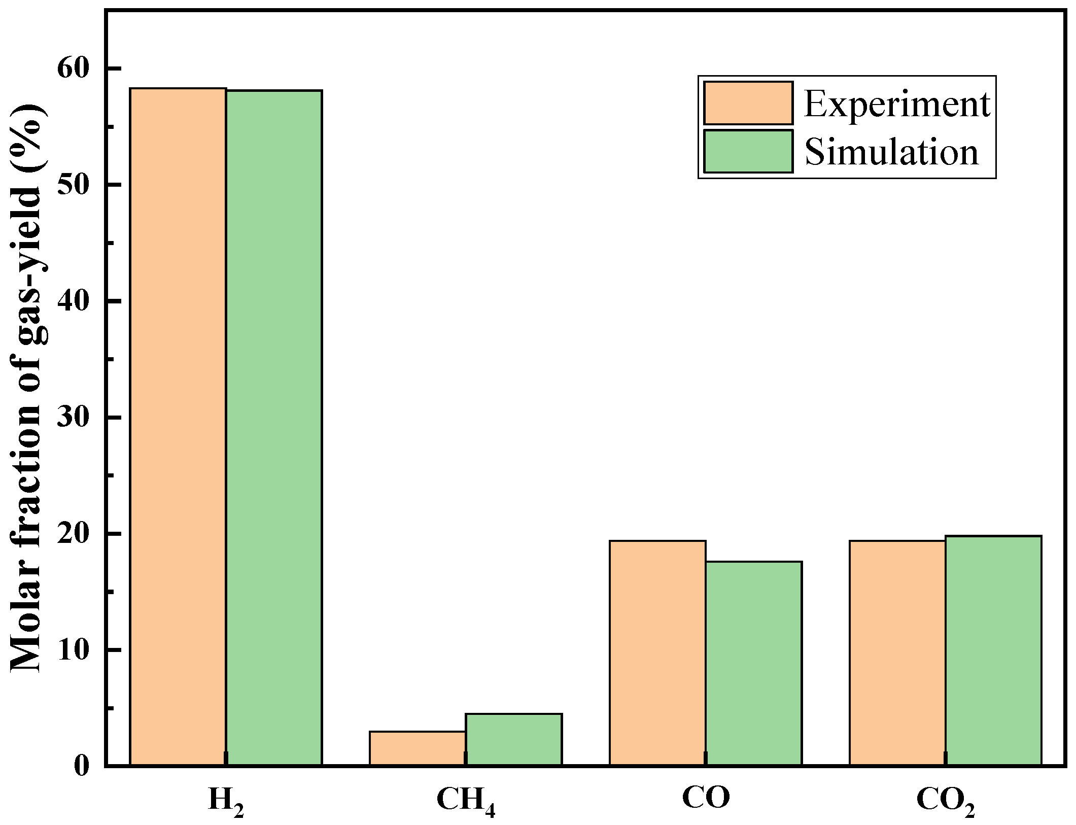
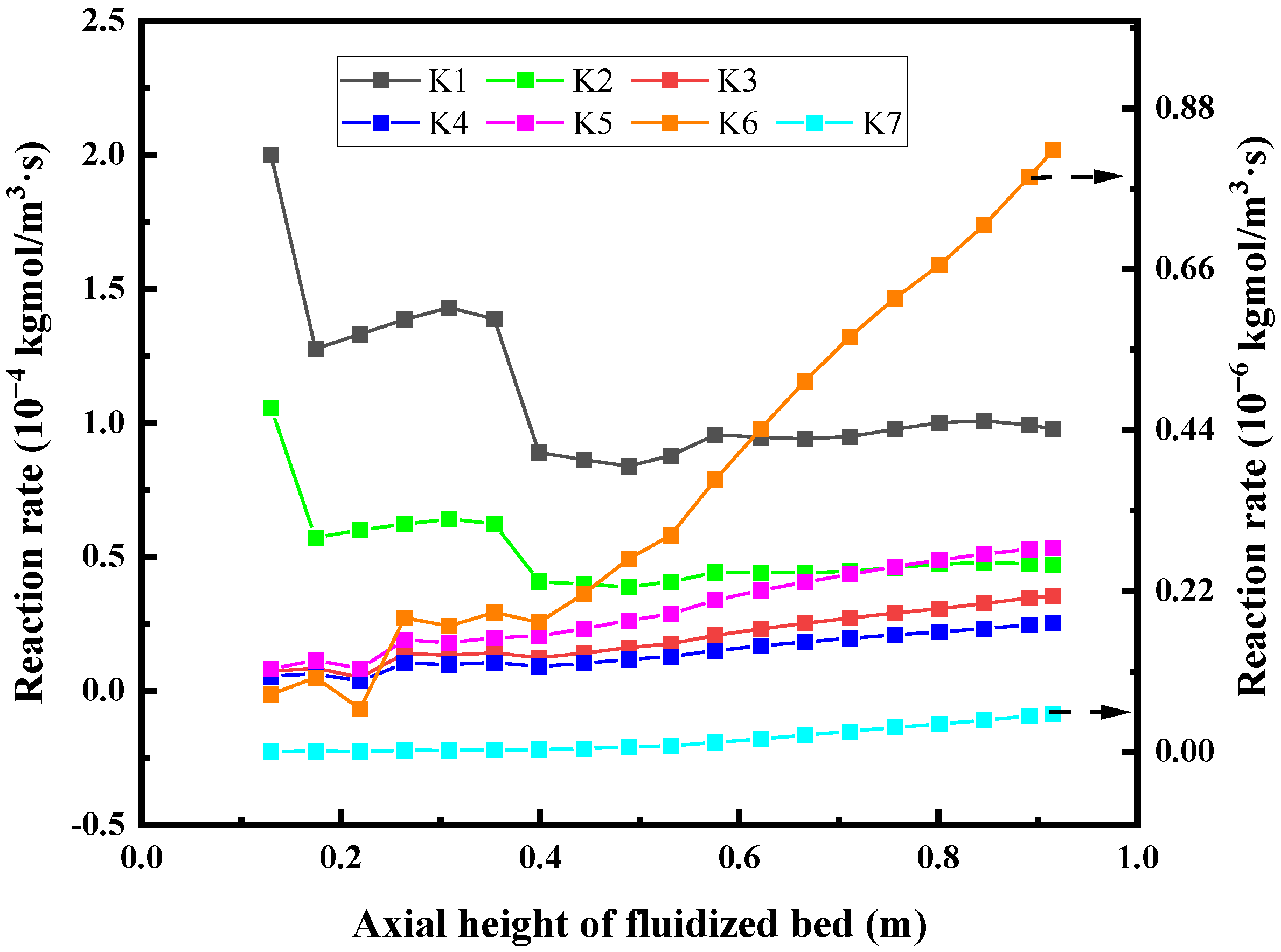
The total thermal effect of supercritical water gasification of glycerol is endothermic. The pyrolysis reaction of glycerol mainly occurs in the middle and lower part of the fluidized bed, while the water gas shift reaction and methanation reaction have the highest reaction rates near the outlet. The production of each gas at the outlet of the fluidized bed increases with the increase of wall temperature.

References

1. Wei, L.; Lu, Y.; Wei, J. Hydrogen production by supercritical water gasification of biomass: Particle and residence time distribution in fluidized bed reactor. Int. J. Hydrogen Energy 2013, 38, 13117–13124. [Google Scholar] [CrossRef]
2. Lu, Y.; Huang, J.; Zheng, P. Fluid hydrodynamic characteristics in supercritical water fluidized bed: A DEM simulation study. Chem. Eng. Sci. 2014, 117, 283–292. [Google Scholar] [CrossRef]
3. Fan, C.; Guo, S.; Jin, H. Numerical study on coal gasification in supercritical water fluidized bed and exploration of complete gasification under mild temperature conditions. Chem. Eng. Sci. 2019, 206, 134–145. [Google Scholar] [CrossRef]
4. Guo, S.; Guo, L.; Cao, C.; Yin, J.; Lu, Y.; Zhang, X. Hydrogen production from glycerol by supercritical water gasification in a continuous flow tubular reactor. Int. J. Hydrogen Energy 2012, 37, 5559–5568. [Google Scholar] [CrossRef]
5. Ostermeier, P.; Fischer, F.; Fendt, S.; DeYoung, S.; Spliethoff, H. Coarse-grained CFD-DEM simulation of biomass gasification in a fluidized bed reactor. Fuel 2019, 255, 115790. [Google Scholar] [CrossRef]
6. Jin, H.; Guo, S.; Guo, L.; Cao, C. A mathematical model and numerical investigation for glycerol gasification in supercritical water with a tubular reactor. J. Supercrit. Fluids 2016, 107, 526–533. [Google Scholar] [CrossRef]
7. Lu, Y.J.; Jin, H.; Guo, L.J.; Zhang, X.M.; Cao, C.Q.; Guo, X. Hydrogen production by biomass gasification in supercritical water with a fluidized bed reactor. Int. J. Hydrogen Energy 2008, 33, 6066–6075. [Google Scholar] [CrossRef]
8. Lu, Y.; Zhao, L.; Han, Q.; Wei, L.; Zhang, X.; Guo, L.; Wei, J. Minimum fluidization velocities for supercritical water fluidized bed within the range of 633–693K and 23–27MPa. Int. J. Multiph. Flow 2013, 49, 78–82. [Google Scholar] [CrossRef]
9. Zou, Z.; Zhao, Y.; Zhao, H.; Li, H.; Zhu, Q.; Xie, Z.; Li, Y. Numerical analysis of residence time distribution of solids in a bubbling fluidized bed based on the modified structure-based drag model. Particuology 2017, 32, 30–38. [Google Scholar] [CrossRef]
10. Li, S.; Zhao, P.; Xu, J.; Zhang, L.; Wang, J. CFD-DEM simulation of polydisperse gas-solid flow of Geldart A particles in bubbling micro-fluidized beds. Chem. Eng. Sci. 2022, 253, 117551. [Google Scholar] [CrossRef]
11. Kalaga, D.V.; Reddy, R.K.; Joshi, J.B.; Dalvi, S.V.; Nandkumar, K. Liquid phase axial mixing in solid–liquid circulating multistage fluidized bed: CFD modeling and RTD measurements. Chem. Eng. J. 2012, 191, 475–490. [Google Scholar] [CrossRef]
12. Wang, S.; Shen, Y. CFD-DEM study of biomass gasification in a fluidized bed reactor: Effects of key operating parameters. Renew. Energy 2020, 159, 1146–1164. [Google Scholar] [CrossRef]
13. Su, X.; Jin, H.; Guo, S.; Guo, L. Numerical study on biomass model compound gasification in a supercritical water fluidized bed reactor. Chem. Eng. Sci. 2015, 134, 737–745. [Google Scholar] [CrossRef]
14. Yao, L.; Lu, Y. Supercritical water gasification of glucose in fluidized bed reactor: A numerical study. Int. J. Hydrogen Energy 2017, 42, 7857–7865. [Google Scholar] [CrossRef]
15. Wu, Y.; Zhang, H.; An, X.; Chen, Z. Numerical investigation on cold flow dynamics of supercritical water fluidized bed reactor with inclined distributor: Design and scale up. Particuology 2022, 67, 90–102. [Google Scholar] [CrossRef]
16. Ostermeier, P.; DeYoung, S.; Vandersickel, A.; Gleis, S.; Spliethoff, H. Comprehensive investigation and comparison of TFM, DenseDPM and CFD-DEM for dense fluidized beds. Chem. Eng. Sci. 2019, 196, 291–309. [Google Scholar] [CrossRef]
17. Lu, Y.; Huang, J.; Zheng, P.; Jing, D. Flow structure and bubble dynamics in supercritical water fluidized bed and gas fluidized bed: A comparative study. Int. J. Multiph. Flow 2015, 73, 130–141. [Google Scholar] [CrossRef]
18. Zhao, L.; Lu, Y. Hydrogen production by biomass gasification in a supercritical water fluidized bed reactor: A CFD-DEM study. J. Supercrit. Fluids 2018, 131, 26–36. [Google Scholar] [CrossRef]
19. Zhang, H.; Huang, Y.; An, X.; Yu, A.; Xie, J. Numerical prediction on the minimum fluidization velocity of a supercritical water fluidized bed reactor: Effect of particle size distributions. Powder Technol. 2021, 389, 119–130. [Google Scholar] [CrossRef]
20. Huang, Y.; Zhang, H.; An, X.; Ye, X. Numerical prediction on minimum fluidization velocity of a supercritical water fluidized bed reactor: Effect of particle shape. Powder Technol. 2022, 403, 117397. [Google Scholar] [CrossRef]
21. Zhang, T.; Lu, Y. Wall-to-bed heat transfer in supercritical water fluidized bed using CFD-DEM. Particuology 2021, 56, 113–123. [Google Scholar] [CrossRef]
22. Zhang, T.; Lu, Y. A method to deal with constant wall flux boundary condition in a fluidized bed by CFD-DEM. Chem. Eng. J. 2021, 406, 126880. [Google Scholar] [CrossRef]
23. Vargas, W.L.; Mccarthy, J.J. Heat conduction in granular materials. Mrs Proc. 2000, 627, 1052–1059. [Google Scholar] [CrossRef]
24. Chaudhuri, B.; Muzzio, F.J.; Tomassone, M.S. Modeling of heat transfer in granular flow in rotating vessels. Chem. Eng. Sci. 2006, 61, 6348–6360. [Google Scholar] [CrossRef]
25. Hertz, H. On the contact of elastic solids. J. Für Die Reine Angew. Math. 1880, 92, 156–171. [Google Scholar]
26. Tsuji, Y.; Kawaguchi, T.; Tanaka, T. Discrete particle simulation of two-dimensional fluidized bed. Powder Technol. 1993, 77, 79–87. [Google Scholar] [CrossRef]
27. Wei, L.; Gu, Y.; Wang, Y.; Lu, Y. Multi-fluid Eulerian simulation of fluidization characteristics of mildly-cohesive particles: Cohesive parameter determination and granular flow kinetic model evaluation. Powder Technol. 2020, 364, 264–275. [Google Scholar] [CrossRef]
28. Lu, Y.; Wei, L.; Wei, J. A numerical study of bed expansion in supercritical water fluidized bed with a non-spherical particle drag model. Chem. Eng. Res. Des. 2015, 104, 164–173. [Google Scholar] [CrossRef]
29. Gidaspow, D. Multiphase Flow and Fluidization: Continuum and Kinetic Theory Descriptions; Academic Press: Cambridge, MA, USA, 1994. [Google Scholar]
30. Guo, S.; Guo, L.; Yin, J.; Jin, H. Supercritical water gasification of glycerol: Intermediates and kinetics. J. Supercrit. Fluids 2013, 78, 95–102. [Google Scholar] [CrossRef]
31. Chen, S.; Fan, Y.; Yan, Z.; Wang, W.; Liu, X.; Lu, C. CFD optimization of feedstock injection angle in a FCC riser. Chem. Eng. Sci. 2016, 153, 58–74. [Google Scholar] [CrossRef]
32. Zhu, L.-T.; Lei, H.; Ouyang, B.; Luo, Z.-H. Using mesoscale drag model-augmented coarse-grid simulation to design fluidized bed reactor: Effect of bed internals and sizes. Chem. Eng. Sci. 2022, 253, 117547. [Google Scholar] [CrossRef]
33. Tripathy, A.; Sahu, A.K.; Biswal, S.K.; Mishra, B.K. A model for expansion ratio in liquid–solid fluidized beds. Particuology 2013, 11, 789–792. [Google Scholar] [CrossRef]
34. Wagner, W.; Cooper, J.R.; Dittmann, A.; Kijima, J.; Kretzschmar, H.J.; Kruse, A.; Mareš, R.; Oguchi, K.; Sato, H.; Stöcker, I. The IAPWS Industrial Formulation 1997 for the Thermodynamic Properties of Water and Steam. J. Eng. Gas Turbines Power 2000, 122, 150–184. [Google Scholar] [CrossRef]
35. Van, W. Fundamentals of Classical Thermodynamics; John Wiley and Sons Ltd.: Hoboken, NJ, USA, 1985. [Google Scholar]
36. Chung, T.H.; Ajlan, M.; Lee, L.L.; Starling, K.E. Generalized multiparameter correlation for nonpolar and polar fluid transport properties. Ind. Eng. Chem. Res. 1988, 27, 671–679. [Google Scholar] [CrossRef]
37. Chao-Hong; He; Yong-Sheng; Yu, New Equation for Infinite-Dilution Diffusion Coefficients in Supercritical and High-Temperature Liquid Solvents. Ind. Eng. Chem. Res. 1998, 37, 3793–3798. [CrossRef]
38. Zbib, H.; Ebrahimi, M.; Ein-Mozaffari, F.; Lohi, A. Hydrodynamic Behavior of a 3-D Liquid-Solid Fluidized Bed Operating in the Intermediate Flow Regime—Application of Stability Analysis, Coupled CFD-DEM, and Tomography. Ind. Eng. Chem. Res. 2018, 57, 16944–16957. [Google Scholar] [CrossRef]
39. Cao, X. Numerical Simulation of Flow and Mixing Characteristics in Tubular Stirred Reactor Using CFD Method. Ph.D. Thesis, Northeastern University, Boston, MA, USA, 2009. [Google Scholar]
Figure 1. Sketch of the fluidized bed.
Energies 15 07128 g001
Figure 2. Relationship between pressure drop and superficial velocities in fluidized bed (25 MPa 699 K).
Energies 15 07128 g002
Figure 3. Comparison between numerical simulation and prediction of minimum fluidization velocity under different temperature and pressure conditions.
Energies 15 07128 g003
Figure 4. Snapshot of particles in the initial stage of fluidization. (Temperature of SCW, 699 K; temperature of feed, 300 K; pressure, 25 MPa; velocity of feed, 0.0262 m/s; velocity of SCW, 0.17 m/s; number of particles, 30,000).
Energies 15 07128 g004
Figure 5. Instantaneous particle velocity vectors. (a) The velocity vector at feed pipe. (b) The velocity vector of the upper and middle sections of the fluidization section. (c) The velocity vector of top of the fluidized bed.
Energies 15 07128 g005
Figure 6. Radial distribution of time-averaged solid volume fraction at different bed heights.
Energies 15 07128 g006
Figure 7. PDF of the solid volume fraction for different initial bed heights.
Energies 15 07128 g007
Figure 8. CDF of the particle volume fraction for different initial bed heights.
Energies 15 07128 g008
Figure 9. PDF of RTD for different initial bed heights.
Energies 15 07128 g009
Figure 10. CDF of RTD for a tubular reactor and fluidized beds with different initial bed heights.
Energies 15 07128 g010
Figure 11. Nonuniformity index and expansion ratio of different initial bed heights.
Energies 15 07128 g011
Figure 12. Structure diagram of different feeding structures.
Energies 15 07128 g012
Figure 13. Instantaneous velocity vectors at the inlet of different feed structures.
Energies 15 07128 g013
Figure 14. PDF of the solid volume fraction of different feeding structures.
Energies 15 07128 g014
Figure 15. CDF of the solid volume fraction of different feeding structures.
Energies 15 07128 g015
Figure 16. Nonuniformity index of different feeding structures.
Energies 15 07128 g016
Figure 17. CDF of RTD at different feeding structures.
Energies 15 07128 g017
Figure 18. Comparison of mole fractions of components in experimental and simulated gas yield.
Energies 15 07128 g018
Figure 19. The temperature distribution of the central axis of the fluidized bed.
Energies 15 07128 g019
Figure 20. The chemical reaction rate is distributed along the axial direction of the fluidized bed.
Energies 15 07128 g020
Figure 21. Axial temperature distribution of fluidized bed under different wall temperatures.
Energies 15 07128 g021
Figure 22. Composition of gas products in fluidized bed under different wall temperatures.
Energies 15 07128 g022