

Methodologies for Synthetic Spatial Building Stock Modelling: Data-Availability-Adapted Approaches for the Spatial Analysis of Building Stock Energy Demand

 ,
,  , ,
, , 
Abstract
:1. Introduction
- Develop and describe data-adapted approaches for generating spatially distributed synthetic building stocks that can be used in building stock modelling in data-scarce circumstances.
- Demonstrate the applications of the developed approaches for spatial synthetic building stock modelling based on two cases: Dublin (Ireland) and Waidhofen an der Thaya (Austria).
- Analyse the spatial distribution of energy demand of the building stock of the two cases based on the application of the approaches.
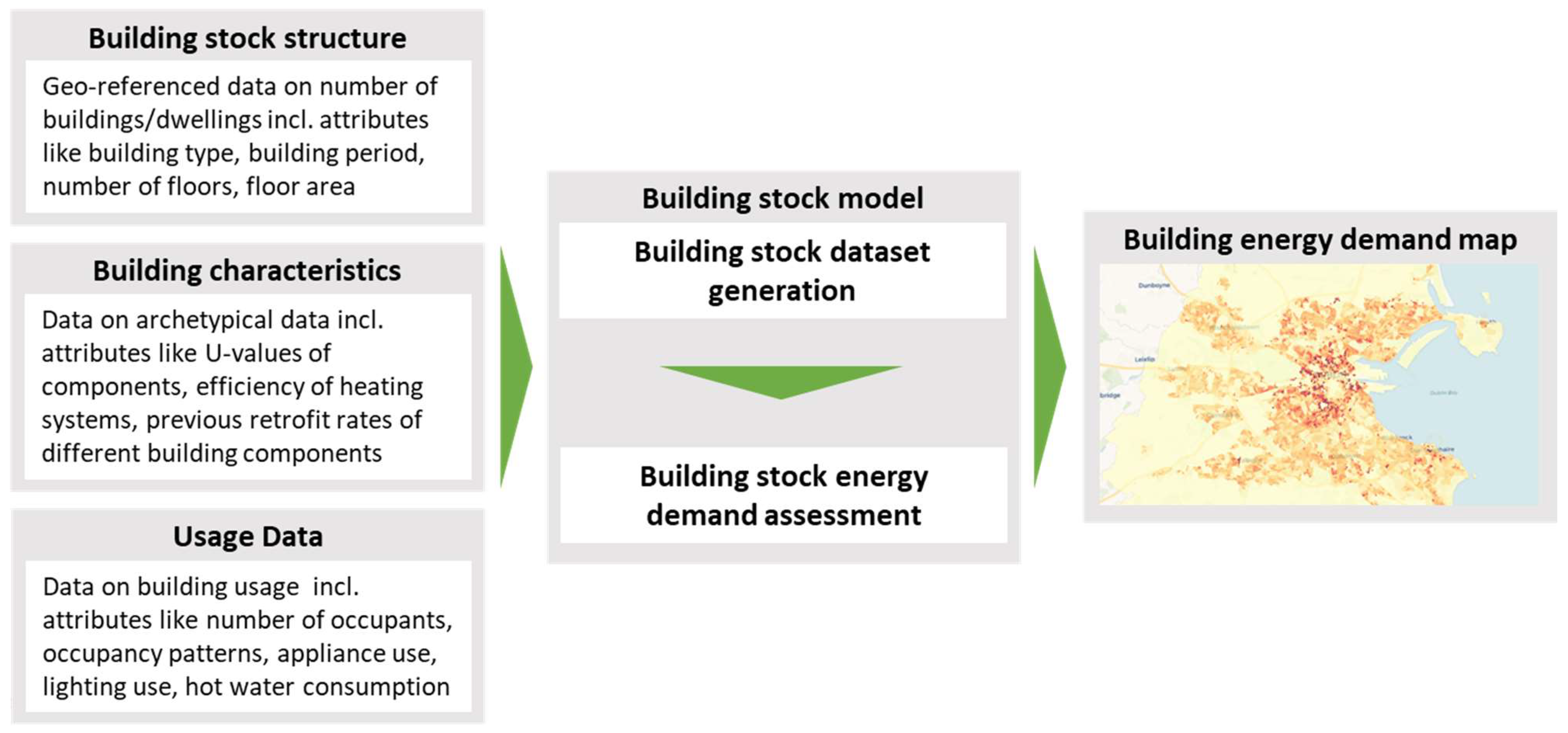
2. Materials and Methods
2.1. Building Stock Dataset Generation
- Building stock initialization: The first step initializes the synthetic building stock resulting in a dataset of individual building records that are spatially distributed. The generated datasets resemble the real building stock both in its structure (e.g., building type, size and age) and spatial distribution. The spatial resolution is determined by the available data and maybe be down to grid-cells or statistical areas;
- Building characterization: The second step further characterizes the individual buildings in the synthetic building stock and enriches the dataset by adding different attributes required for building stock energy modelling. These may include estimating the building geometry, assigning heating and ventilation systems and energy-relevant parameters (e.g., U-values). This may include stochastically assigning attributes based on distributions or assigning data based on archetype data;
- Updating building characteristics: The third step updates individual building characteristics to better represent the current state of the stock (e.g., in terms of current U -values) to account for past retrofits and other alterations. This step may be unnecessary in case the data used for step 2 is up to date.
2.1.1. Sample-Based SBSEM
2.1.2. Sample-Free SBSEM
2.2. Building Stock Energy Demand Assessment
2.3. Validation
2.4. Cases
2.4.1. Dublin (Ireland)
Building Stock Initialization
Building Stock Characterization
2.4.2. Waidhofen an der Thaya (Austria)
Building Stock Initialization
Building Stock Characterization
3. Results
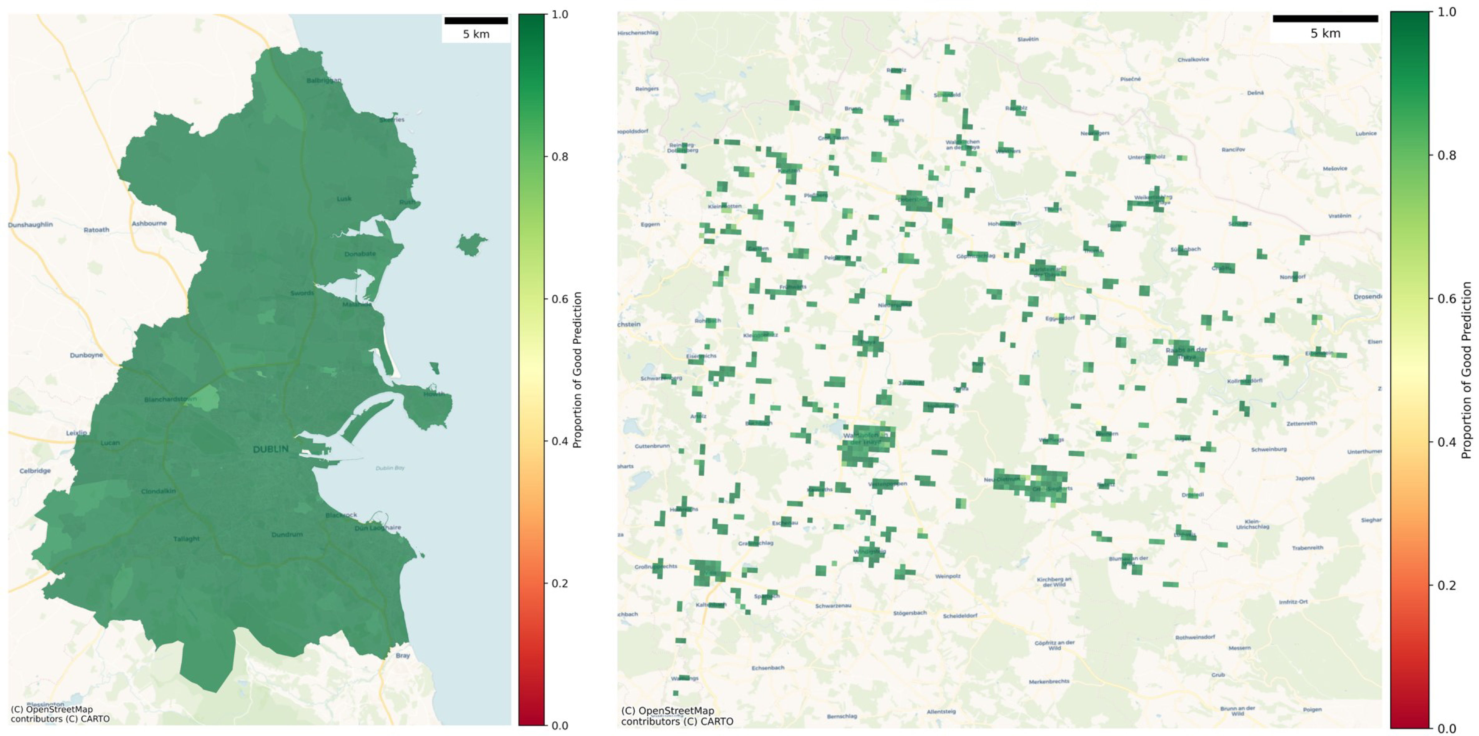
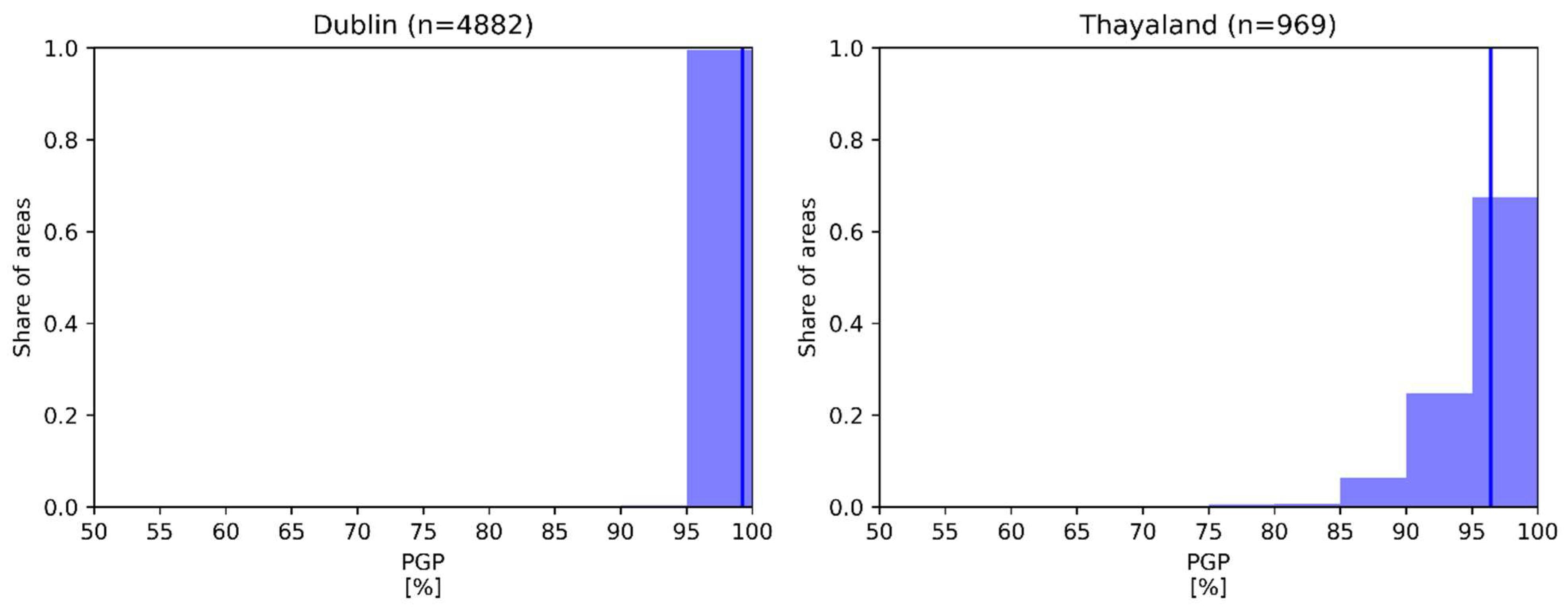
3.1. Validation
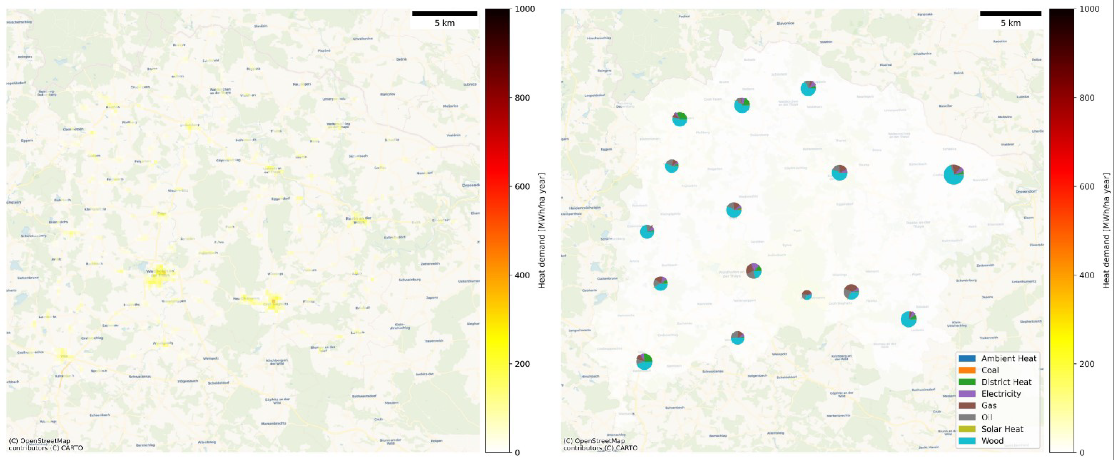
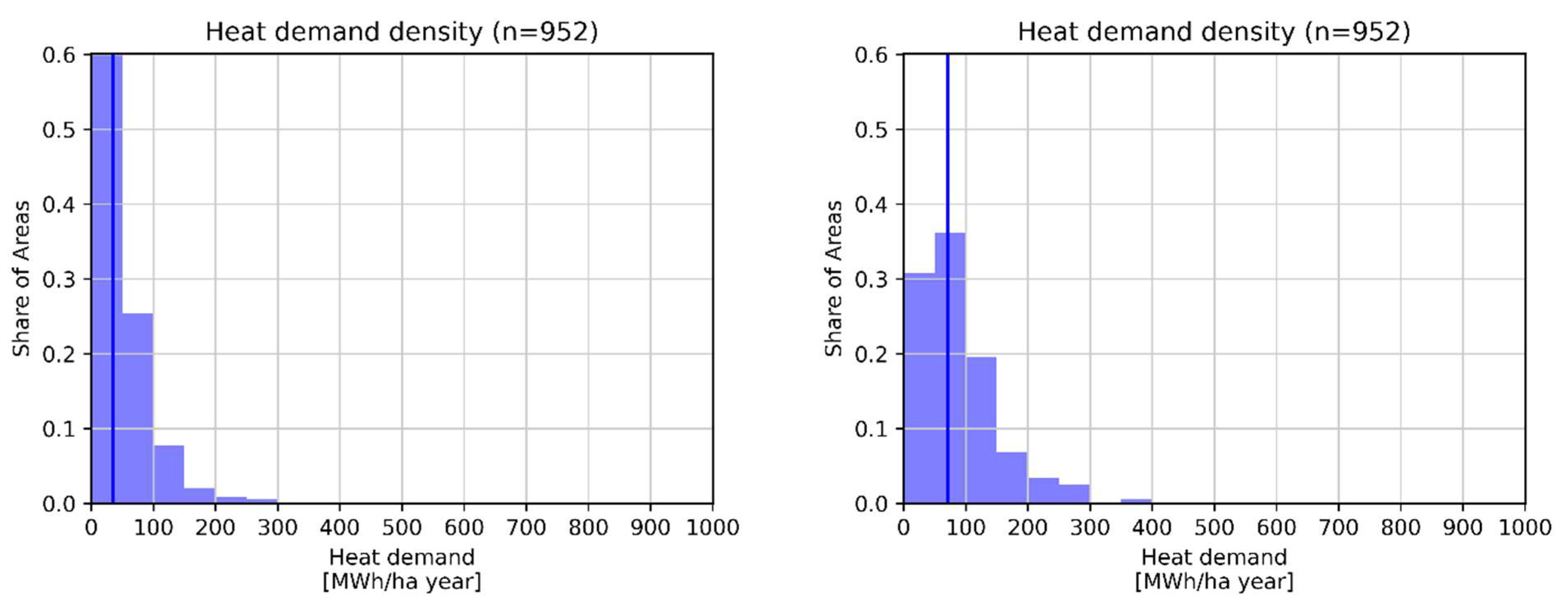
3.2. Distribution of Energy Demand
3.2.1. Dublin
3.2.2. Waidhofen
4. Discussion
5. Conclusions
Author Contributions
Funding
Acknowledgments
Conflicts of Interest
References
- European Commission Factsheet: The Energy Performance of Buildings Directive. 2017. Available online: https://ec.europa.eu/energy/sites/ener/files/documents/buildings_performance_factsheet.pdf (accessed on 13 September 2020).
- Kavgic, M.; Mumovic, D.; Summerfield, A.; Stevanovic, Z.; Ecim-djuric, O. Uncertainty and Modeling Energy Consumption: Sensitivity Analysis for a City-Scale Domestic Energy Model. Energy Build. 2013, 60, 1–11. [Google Scholar] [CrossRef]
- Langevin, J.; Reyna, J.L.; Ebrahimigharehbaghi, S.; Sandberg, N.; Fennell, P.; Nägeli, C.; Laverge, J.; Delghust, M.; Mata, É.; Van Hove, M.; et al. Developing a Common Approach for Classifying Building Stock Energy Models. Renew. Sustain. Energy Rev. 2020, 133, 110276. [Google Scholar] [CrossRef]
- Nägeli, C.; Jakob, M.; Catenazzi, G.; Ostermeyer, Y. Policies to Decarbonize the Swiss Residential Building Stock: An Agent-Based Building Stock Modeling Assessment. Energy Policy 2020, 146, 111814. [Google Scholar] [CrossRef]
- Sandberg, N.H.; Næss, J.S.; Brattebø, H.; Andresen, I.; Gustavsen, A. Large Potentials for Energy Saving and Greenhouse Gas Emission Reductions from Large-Scale Deployment of Zero Emission Building Technologies in a National Building Stock. Energy Policy 2021, 152, 112114. [Google Scholar] [CrossRef]
- Kranzl, L.; Hummel, M.; Müller, A.; Steinbach, J. Renewable Heating: Perspectives and the Impact of Policy Instruments. Energy Policy 2013, 59, 44–58. [Google Scholar] [CrossRef]
- Fonseca, J.A.; Nguyen, T.; Schlueter, A.; Marechal, F. City Energy Analyst (CEA): Integrated Framework for Analysis and Optimization of Building Energy Systems in Neighborhoods and City Districts. Energy Build. 2016, 113, 202–226. [Google Scholar] [CrossRef]
- Österbring, M.; Nägeli, C.; Camarasa, C.; Thuvander, L.; Wallbaum, H. Prioritizing Deep Renovation for Housing Portfolios. Energy Build. 2019, 202, 109361. [Google Scholar] [CrossRef]
- Reinhart, C.F.; Cerezo Davila, C. Urban Building Energy Modeling—A Review of a Nascent Field. Build. Environ. 2016, 97, 196–202. [Google Scholar] [CrossRef]
- Mastrucci, A.; Marvuglia, A.; Leopold, U.; Benetto, E. Life Cycle Assessment of Building Stocks from Urban to Transnational Scales: A Review. Renew. Sustain. Energy Rev. 2017, 74, 316–332. [Google Scholar] [CrossRef]
- Österbring, M.; Mata, É.; Thuvander, L.; Mangold, M.; Johnsson, F.; Wallbaum, H. A Differentiated Description of Building-Stocks for a Georeferenced Urban Bottom-up Building-Stock Model. Energy Build. 2016, 120, 78–84. [Google Scholar] [CrossRef] [Green Version]
- Mangold, M.; Österbring, M.; Wallbaum, H. Handling Data Uncertainties When Using Swedish Energy Performance Certificate Data to Describe Energy Usage in the Building Stock. Energy Build. 2015, 102, 328–336. [Google Scholar] [CrossRef]
- Nägeli, C.; Camarasa, C.; Jakob, M.; Catenazzi, G.; Ostermeyer, Y. Synthetic Building Stocks as a Way to Assess the Energy Demand and Greenhouse Gas Emissions of National Building Stocks. Energy Build. 2018, 173, 443–460. [Google Scholar] [CrossRef]
- Beckman, R.J.; Baggerly, K.A.; McKay, M.D. Creating Synthetic Baseline Populations. Transp. Res. Part A Policy Pract. 1996, 30, 415–429. [Google Scholar] [CrossRef]
- Nägeli, C.; Jakob, M.; Catenazzi, G.; Ostermeyer, Y. Towards Agent-Based Building Stock Modeling: Bottom-up Modeling of Long-Term Stock Dynamics Affecting the Energy and Climate Impact of Building Stocks. Energy Build. 2020, 211, 109763. [Google Scholar] [CrossRef]
- Lenormand, M.; Deffuant, G. Generating a Synthetic Population of Individuals in Households: Sample-Free vs. Sample-Based Methods. J. Artifical Soc. Soc. Simul. 2013, 16, 1–10. [Google Scholar] [CrossRef]
- Ye, X.; Konduri, K.; Pendyala, R.M.; Sana, B.; Waddel, P. A Methodology To Match Distributions of Both Household and Person Attributes in the Generation of Synthetic Populations. 88th Annu. Meet. Transp. Res. Board 2011, 9600, 1–25. [Google Scholar]
- Moeckel, R.; Spiekermann, K.; Wegener, M. Creating a Synthetic Population. In Proceedings of the 8th International Conference on Computers in Urban Planning and Urban Management (CUPUM), Sendai, Japan, 27 May 2003; pp. 1–18. [Google Scholar]
- Gargiulo, F.; Ternes, S.; Huet, S.; Deffuant, G. An Iterative Approach for Generating Statistically Realistic Populations of Households. PLoS ONE 2010, 5, e8828. [Google Scholar] [CrossRef] [PubMed]
- Nägeli, C.; Farahani, A.; Österbring, M.; Dalenbäck, J.O.; Wallbaum, H. A Service-Life Cycle Approach to Maintenance and Energy Retrofit Planning for Building Portfolios. Build. Environ. 2019, 160, 106212. [Google Scholar] [CrossRef]
- ISO 52016-1; Energy Performance of Buildings—Energy Needs for Heating and Cooling, Internal Temperatures and Sensible and Latent Heat Loads—Part 1: Calculation Procedures 2017. ISO: Geneva, Switzerland, 2017.
- CSO Regional Population Projections. Available online: https://www.cso.ie/en/statistics/population/regionalpopulationprojections/ (accessed on 25 January 2022).
- European Parliament Directive 2010/31/EU of the European Parliament and of the Council of 19 May 2010 on the Energy Performance of Buildings (Recast). Off. J. Eur. Union 2010, 53, 13–35. [CrossRef]
- Goverment of Ireland. Ireland’s Long-Term Renovation Strategy 2020; Goverment of Ireland: Dublin, Ireland, 2020.
- CSO Census 2016 Reports. Available online: https://www.cso.ie/en/census/census2016reports/ (accessed on 12 November 2020).
- SEAI BER Public Search. Available online: https://ndber.seai.ie/BERResearchTool/Register/Register.aspx (accessed on 12 November 2020).
- UDST UDST/Synthpop: Synthetic Populations from Census Data. Available online: https://github.com/UDST/synthpop (accessed on 1 November 2021).
- eKUT. Regional Energy Demand Analysis Portal: Thermal Energy Consumption in Thayaland Region; eKUT: Waidhofen/Thaya, Austria, 2021. [Google Scholar]
- KEM Energiezukunft Thayaland: Klima-Und Energie-Modellregionen. Available online: https://www.klimaundenergiemodellregionen.at/modellregionen/liste-der-regionen/getregion/32 (accessed on 25 January 2022).
- Statistics Austria. Regional Statsitics-Package Buildings and Dwellings Register; Statistics Austria: Vienna, Austria, 2020. [Google Scholar]
- Statistics Austria. Package Census 2011-Workplace/Local Units of Employment; Statistics Austria: Vienna, Austria, 2020. [Google Scholar]


| Nr. | Dataset | Description | Spatial Resolution | Attributes | Source |
|---|---|---|---|---|---|
| 1 | Census of Population | Dataset describing the spatial distribution of dwellings per statistical area (small area) | Small area | Number of dwellings per construction period, building type and energy carrier for heating | [25] |
| 2 | National building energy rating (BER) Research Tool | Energy performance certificate database of Ireland containing data on dwellings with an energy performance certificate | Postcode | Postcode, building type, construction year, floor area, component surface area, component-U-values, heating and hot water systems, ventilation type | [26] |
| Nr. | Dataset | Description Dataset | Spatial Resolution | Attributes | Source |
|---|---|---|---|---|---|
| 1 | Building and dwelling registry–grid 250 m | Dataset describing the spatial distribution of number of buildings and dwellings | 250 × 250 raster grid | Number of buildings per building type, construction period, size and number of dwellings Number of dwellings per size and number of rooms | [30] |
| 2 | Register-based Census 2011-Housing Census | Dataset describing the composition and structure of the building and dwelling stock | Entire region | Number of buildings per building type, construction period, size and number of dwellings Number of dwellings per size and number of rooms | [31] |
| 3 | Survey study | Overview study of building stock in Waidhofen | Municipality | Building type, construction year, U-value and heating system distribution | [28] |
Publisher’s Note: MDPI stays neutral with regard to jurisdictional claims in published maps and institutional affiliations. |
© 2022 by the authors. Licensee MDPI, Basel, Switzerland. This article is an open access article distributed under the terms and conditions of the Creative Commons Attribution (CC BY) license (https://creativecommons.org/licenses/by/4.0/).
Share and Cite
Nägeli, C.; Thuvander, L.; Wallbaum, H.; Cachia, R.; Stortecky, S.; Hainoun, A. Methodologies for Synthetic Spatial Building Stock Modelling: Data-Availability-Adapted Approaches for the Spatial Analysis of Building Stock Energy Demand. Energies 2022, 15, 6738. https://doi.org/10.3390/en15186738
Nägeli C, Thuvander L, Wallbaum H, Cachia R, Stortecky S, Hainoun A. Methodologies for Synthetic Spatial Building Stock Modelling: Data-Availability-Adapted Approaches for the Spatial Analysis of Building Stock Energy Demand. Energies. 2022; 15(18):6738. https://doi.org/10.3390/en15186738
Chicago/Turabian StyleNägeli, Claudio, Liane Thuvander, Holger Wallbaum, Rebecca Cachia, Sebastian Stortecky, and Ali Hainoun. 2022. "Methodologies for Synthetic Spatial Building Stock Modelling: Data-Availability-Adapted Approaches for the Spatial Analysis of Building Stock Energy Demand" Energies 15, no. 18: 6738. https://doi.org/10.3390/en15186738
APA StyleNägeli, C., Thuvander, L., Wallbaum, H., Cachia, R., Stortecky, S., & Hainoun, A. (2022). Methodologies for Synthetic Spatial Building Stock Modelling: Data-Availability-Adapted Approaches for the Spatial Analysis of Building Stock Energy Demand. Energies, 15(18), 6738. https://doi.org/10.3390/en15186738