Valuation of the Extension Option in Time Charter Contracts in the LNG Market

Abstract

A rapid transition toward a decarbonized economy is underway, following the Paris Agreement and the International Maritime Organization 2030 decarbonization goals. However, due to the high cost of the rapid transition to eco-friendly energy and the geopolitical conflict in eastern Europe, liquefied natural gas (LNG), which emits less carbon than other fossil fuels, is gaining popularity. As the spot market grows due to increased LNG demand, the usage of period extension options in time charter (T/C) contracts is increasing; however, these options are generally provided free of charge in practice, without economic evaluation; this is because some shipowners want to make their time charter contracts more attractive to the more credible charterers. Essentially, the reason for why this option has not been evaluated is because there is no reliable evaluation model currently used in practice. That is, research on the evaluation model for the T/C extension option has been insufficient. Therefore, this study evaluates the economic value of the extended period option in LNG time charter contracts using machine learning models, such as artificial neural networks, support vector machines, and random forest, and then compares them with the Black–Scholes model that is used for option valuations in financial markets. The results indicate superior valuation performance of the random forest model compared with the other models; particularly, its performance was significantly better than the Black–Scholes model. Since T/C extension options involve significant sums in the balance sheets of both shipowners and charterers, the fair value of these options should be assessed. In this regard, this paper has meaning in proposing valid machine models to efficiently reflect the fair value of period extension options that are provided at no charge in the LNG market.

1. Introduction

1.1. Background of the Study

Suppliers and consumers are “pre-specialized projects” that form a binding relationship through mutual cooperation, because liquefied natural gas (LNG) projects are linked to LNG value chains, which in turn are linked to exploration, liquefaction, sea transportation, regeneration, and consumption, through long-term and large-scale finances. Unlike other dry bulk ship markets, shippers, also referred to as consumers, had to transport cargo through LNG carriers that were suitable for a designated port based on take or pay for contract volume with suppliers; therefore, shippers had a limited free market [1]. However, as of 2021, the global demand for LNG has been fluctuating, owing to the increased production of shale gas in the United States (U.S.); the onset of commercial production in the Gorgon LNG project in Australia increased LNG supply factors such as the declaration of carbon neutrality in 2060, and the U.S. re-subscribed to the Paris Agreement [2].

The traditional market for global demand and supply for LNG is generally based on long-term contracts. However, owing to the emergence of recently diversified suppliers and massive demand, short-term charter contracts of LNG trading have increased [3].

The LNG time charter (T/C) contract is formed on the basis of an agreement that the shipowner will charter out the LNG carrier to the charterer for a certain period with the crew, which is employed by the shipowner and paid for by the charterer, who boards the ship. In other words, a charterer who charters an LNG carrier is given the status of a carrier, and generates profits by utilizing the chartered ship for maritime transportation [4]. In this case, in the LNG transport contract, the triangular structure of the shipowner, the charterer, and the shipper, forms a relationship. Since the LNG periodic charter contracts are provided by the ship owners, and only operated by the regular charterers, they may vary depending on the subject of each cost-sharing or responsibility, especially the option to extend the charter period. In order to solve this problem, Shell LNG Time 1 (developed in 2005) and Shell LNG Time 2 (developed in 2016), which were developed by the Baltic and International Maritime Council, are used as long-term charter-based standard contracts [5]. The reason for this is because the shipowner is required to balance the risk and reward with charterers, based on long-term charters for expensive LNG carriers that cost about $275 million, according to the Clarkson Newbuilding Price Index in 2021. In fact, unlike ShellTime, ShellLNGTime1 considers (1) the right to choose the boil-off gas (BOG), (2) the ship-to-ship (STS) problem within the charter period, and (3) the extension of the charter period due to market fluctuations as key issues, and constitutes the contract clause. Since the introduction of the world’s first dual-fuel diesel-electric (DFDE) LNG vessel in 2006, charterers have decided whether to exercise the option to extend the charter period, depending on whether the vessel is installed or not [6].

In practice, if it is recognized that the charter period is exceeded or shortened, the excess or shortened period is referred to as the allowable period of the charter period, while the basic charter period and extension options are highly diverse, as shown in

Table 1. Chartering period and option to extend for LNG T/C.

Chartering Period	Option to Extend	Remark
3~5 M (month)	(±) 15 days
4~6 M (month)	(±) 15 days
6~8 M (month)	(±) 15 days
12 M	1 Month	about (±) 15 days
24 M	2 Month	about (±) 15 days
36 M	6 Month	about (±) 30 days

Source: Based on interviews with LNG chartering experts.

below [7,8]. Therefore, for a time charterer, (1) selecting whether the allowable period for the charter period is recognized and (2) the criteria for determining the payment of the charter fee at this time, are essential factors in selecting the LNG charter period for a shipping company. In particular, it is very important for shipowners and charterers to predict how to agree on a fixed period, optional period, and flexible period of acceptance, based on a periodic charter contract that considers future LNG market conditions [9].

Typically, the LNG time charterers often have the option of extending the T/C period at the same freight rate as that of the original contract, which can result in a unilateral transfer of profits to the time charterers. If such an option for extension is specified in the LNG charter contract, the time charterer does not exercise the option to extend the charter period if the LNG transportation market is weak, which results in an imbalance in the shipowner’s efforts to sign a new contract with a new charterer. Alternatively, if the LNG transportation market is booming, the time charterer can actively exercise the extension option in order to maximize profits by operating the ship using low charter rates, and the shipowner receives a charter fee that is lower than the market price [10]. In order to minimize the key issues in dispute, with the option to extend the charter period, the LNG shipowners can sign a periodic charter contract with the charter companies Chevron, Exxon, British Petroleum, and Royal Dutch Shell, which focus on DFDE-based LNG vessels, and extend the charter period once every three months.

1.2. Research Aim

The global shipping industry must comply with International Maritime Organization (IMO) green-house-gas (GHG) regulations that require a 40% reduction by 2030 in carbon emissions, and a 70% reduction by 2050 from base year 2008 [11]. This requires shipping companies to carry out eco-friendly initiatives, such as replacing fleets with new LNG-fueled ships, changing to clean fuel, adopting energy saving devices, and reducing ships’ transport speed.

In particular, to support the carbon neutrality policy of global shipping companies, a periodic charter contract should be prepared for spot cargo due to the increased demand for LNG as a bridge fuel, before non-carbon fuels such as hydrogen and ammonia are commercialized. Therefore, this study suggests an optimal plan by examining whether the charterer will give up the right to choose to extend the charter period after the end of the LNG vessel period, or how it changes depending on market fluctuations. In particular, this study only used the Black–Scholes model to evaluate the economic value of extension options in general charter contracts. However, this study aims to strengthen the competitiveness of shipping companies by comprehensively comparing machine learning models such as artificial neural networks, support vector regression, and random forest models.

In the shipping market, constant efforts are being made to apply fourth industrial revolution technology to the field. In particular, countries worldwide are racing to develop the world’s first autonomous ships. This phenomenon is limited to the technical aspects. Evidently, hardware innovation is necessary, but it is also necessary to improve the quality of decision making in the shipping industry. However, most of the studies that use machine learning (ML) methods for shipping market problems focus on the Baltic Dry Index (BDI) for forecasting sea traffic. Li and Parsons [12] suggested the use of an artificial neural network (ANN)-based framework in forecasting tanker freight rate, and showed better performance of using an ANN compared to ARMA (autoregressive moving averages). Mostafa [13] presented an ANN’s possibility to estimate the traffic volume of the Suez Canal. Yang et al. [14] proposed using an early warning system with support vector machine (SVM) for the container and dry bulk freight rates in the shipping market. Fan et al. [15] built an ANN with a wavelet function as the activation function, obtaining important information from noisy data. Lyridis et al. [16] devised an ANN model to forecast the forward freight agreement (FFA) prices, and Santos et al. [17] developed a radial basis function (RBF)-based ANN to predict the time charter rate of VLCC. Han et al. [18], Daranda [19], and Bao et al. [20] employed an SVM and ANN to estimate the Baltic Dry Index, and they concluded that there is availability of and applicability for machine learning in the shipping market. Therefore, this study attempts to apply ML models such as ANN, SVM, and random forest (RF) to LNG shipping market decisions, especially charter-related decisions. The primary objective of these studies is to evaluate the option to extend the period in LNG time-charter contracts (T/C extension options) with ML methods, and provide an improved framework for the decision making in shipping chartering practices. 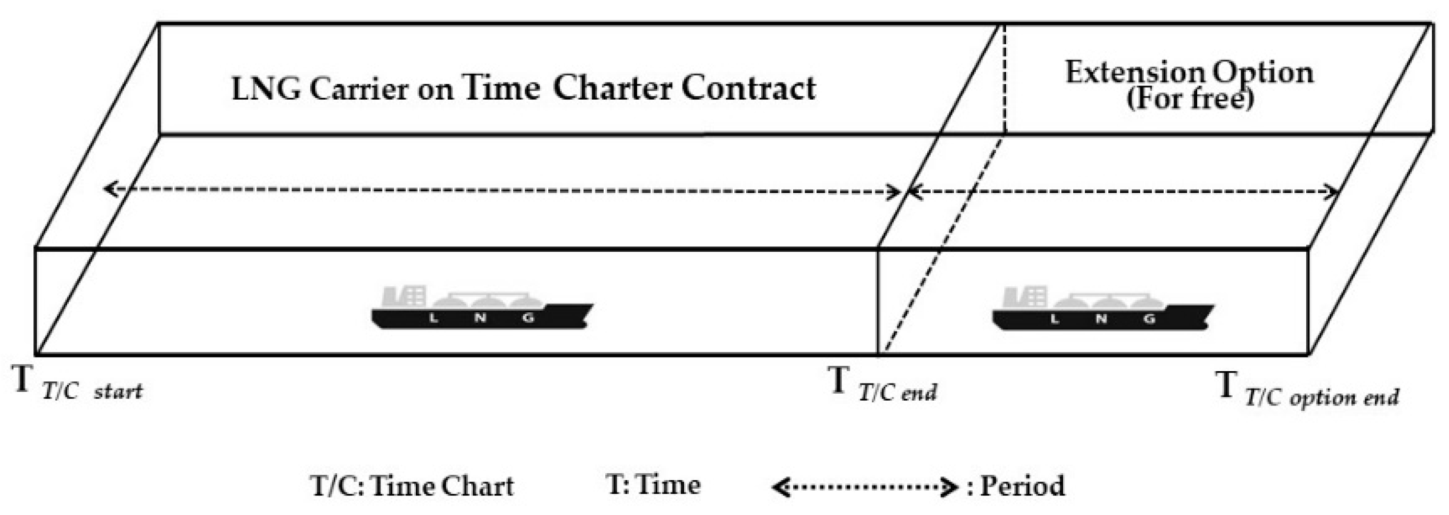Alizadeh and Nomikos [7] mentioned that the T/C extension option is embedded in the time charter party. These options are involved in an original T/C contract, and they are exercised at the end of the pre-specified period of the contract in order to extend its period; moreover, the charterer can maintain the same rates as the original contract. However, since these T/C options are provided to the charterer at no cost instead of imposing fair value, these unknown values may prove advantageous for the charterer. Figure 1 shows the structure of the T/C extension option in the contract.

The purpose of providing T/C extension options at no cost is to attract charterers with more credibility in the very competitive shipping market, and maintain close relationships with them [7,8,10]. After the financial crisis, the shipping market collapsed because of the world economic recession. The large volume of shipbuilding orders placed during the shipping boom period resulted in excess carrying capacities, and hampered the recovery of the shipping freight market. Shipowners with expensive fleets that were built during the bull market, and the charterers that borrowed ships at a high rate, have been harassed due to the crash of the LNG shipping freight market. Under the bearish market, shipowners began to give T/C extension options to counterparties for free, in order to attract charterers in the LNG market who had higher credibility. Therefore, this study priced the 3-month T/C options that are embedded in their 1-year mother contracts, especially in the LNG shipping market sector.

2. Data and Methodologies

2.1. Data

The data used in this paper were the spot and T/C of LNG carriers with a size of 160,000 m³, including the US T-bill rate obtained from Shipping Intelligence Networks [21] and their descriptive statistics are in

Table 2. Descriptive statistics of the data.

Stat.	LNG 160,000 m3 Spot ($/day)	LNG 160,000 m3 1 yr T/C ($/day)	US-TB (%)
Average	73,934.24	74,186.55	0.009742
Standard Deviation	38,816.69	33,166.08	0.007855
Kurtosis	0.270679	−0.4441	−0.23805
Skewness	0.850399	0.485316	1.017874
Observation	595	595	595
Period	7 January 2011~27 May 2022

. The size of LNG carriers is divided into 145,000 m³, 160,000 m³, and 174,000 m³, based on cargo volume. The reason other carriers were not used despite their sizes, which are 145,000 m³ and 174,000 m³ in the case of the LNG freight market, is because their freight time series data are not sufficiently long. The volatility in the LNG shipping market has recently increased due to political issues; it used to be a low-volatility market, with relatively inactive spot trading. Since most of the volume is based on long-term transactions, freight volatility and diversity are lower than in other markets. The first three months of the freight data were used for calculating the annualized volatility of the rate, and the last year was used for the actual value of the extension option.

As there is no three-month freight rate in the LNG market, this paper used the spot rate of 160,000 m³ freight rate as the proxy for the three-month rate. As mentioned earlier, due to the freight characteristics of the LNG market, this did not seriously affect the research results.

2.2. Methodologies

2.2.1. Black–Scholes Model

The Black–Scholes option pricing model (BSM), first introduced by Black, Scholes, and Merton, has been used for option valuations in the financial market [22,23,24]. Owing to the tractability and simplicity of this model, it is still widely accepted as the benchmark model [25,26,27,28]. Equations (1) and (2) describe the parameters of the BSM:

$$\mathrm{C}=S_{0}N\left(d_1\right)-K{e}^{-rT}N\left(d_2\right),$$

(1)

$$d_1=\frac{\ln \left(\frac{S_0}{K}\right)+\left(r+\frac{{\sigma }^2}{2}\right)T}{\sigma \sqrt{T}} ,d_2=d_1-\sigma \sqrt{T},$$

(2)

where $\mathrm{C}$ is the European call option price, $S_0$ is the spot price at time 0, $K$ is the strike price, $N(\bullet )$ is the cumulative probability distribution function with a standard normal distribution, $r$ is the risk-free rate, $\sigma$ is the spot price volatility, and $T$ is the time to maturity of the option.

According to Yun et al. [8], to apply the BSM model to the valuation of T/C extension option, the premise that the extension option has the same structure as a European option should be needed. The premises are as follows: (1) the redelivery flexibility of the chartered vessel is ignored; (2) there is no time lag between the contract and the delivery of the vessel; (3) the prices between the option period and the firm period are equal; (4) the exercise of the option is only limited at maturity of the contract; and (5) when exercising, the payoff of the option is based on a 3-month T/C rate at maturity in the LNG contract. These premises enable us to evaluate the T/C extension option in the LNG contract.

There are five parameters of the BSM, which are as follows: LNG spot price, strike price, time to maturity, risk-free rate, and spot return volatility to value the T/C extension option in the LNG contract. Since the volatility of the underlying asset is unknown, this study uses the return of the 3-month T/C rate for one year in order to yield the equally weighted historical volatility, as shown in

Table 3. Parameters of the BSM.

Variables		Data
S	Underlying asset price	LNG 160,000 m3 Spot rate
X	Strike price	LNG 160,000 m3 1 yr-T/C rate
r	Risk-free rate	90-day T-bill
$\sigma$	Volatility of return for underlying asset price	1-year standard deviation of spot rate
T	Time to maturity	1 year

.

Although the ML approach does not require any assumptions [29,30,31,32] especially for the stationarity of the data, the lack of an economic background makes it very difficult to draw meaningful results [33]. Therefore, in order to avoid this drawback in the ML models, the types of input variables are set to be the same as those of the BSM, except for the time to maturity. Instead of the time to maturity, the spot rate is randomly added to reflect the market dynamics.

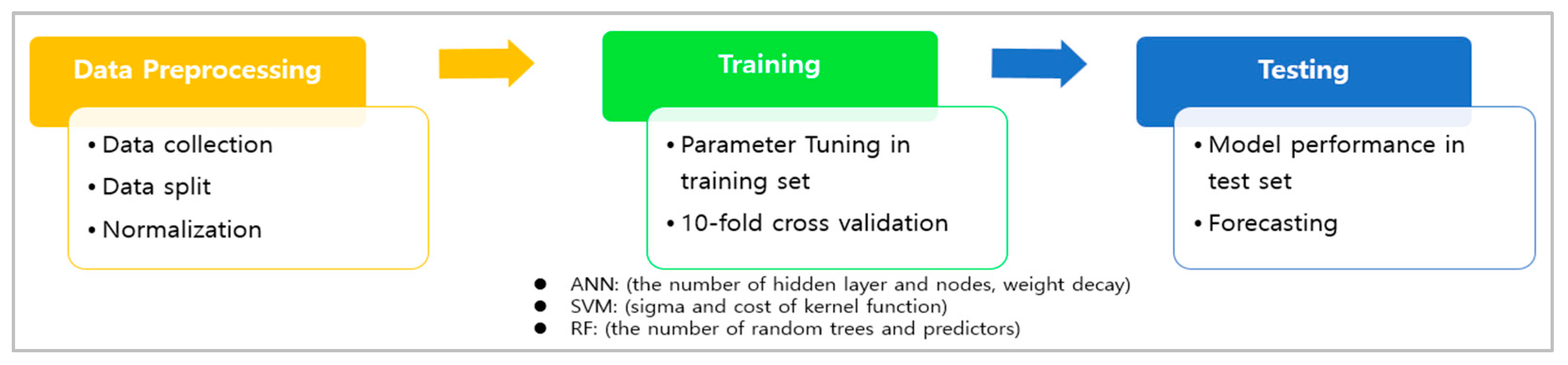
The parameters in the machine learning models should be optimized through the modelling process, as shown in Figure 2.

2.2.2. Artificial Neural Network Model

The artificial neural network (ANN) method artificially constructs the human learning process by modeling the biological neural signal transduction system; such mathematical models have appeared since the 1950s. ANNs are used in various fields, such as accounting, credit rating, decision support, derivatives pricing, and bankruptcy [34]. In the forward process of the hidden node, every input of each node is $ne{t}_j={{\displaystyle \sum }}_i{x}_i{w}_{ji}$, where $x_i$ denotes inputs and $w_{i,j}$ denotes the connection weights between the input node I and the hidden node j. The outcome through the sigmoidal activation function $g\left(ne{t}_j\right)=\frac{1}{1+e^{-\left(ne{t}_j\right)}}$ is the input of output layer $ne{t}^o={{\displaystyle \sum }}_{j}g\left(ne{t}_j\right)w_j^o$. The predicted value ${\mathrm{y}}^o$ is obtained by using the activation function $g\left(ne{t}^o\right)$ again. The gradient descent, referred to as backpropagation learning algorithm in the ANN, is adopted to adjust the connection weights $w$ in order to optimize the total error $E=\frac{1}{2}{\displaystyle \sum }_j{\left({\mathrm{y}}^a-{\mathrm{y}}^o\right)}^2$, where ${\mathrm{y}}^a$ denotes the actual value. The following Equations (3) and (4) are the weight adjustments in backpropagation process:

$$∆w_j^{o }=\eta {\delta }^{o}g\left(ne{t}^o\right)$$

(3)

$$∆w_{i,j}=\eta {\delta }_{j}g\left(ne{t}_j\right)$$

(4)

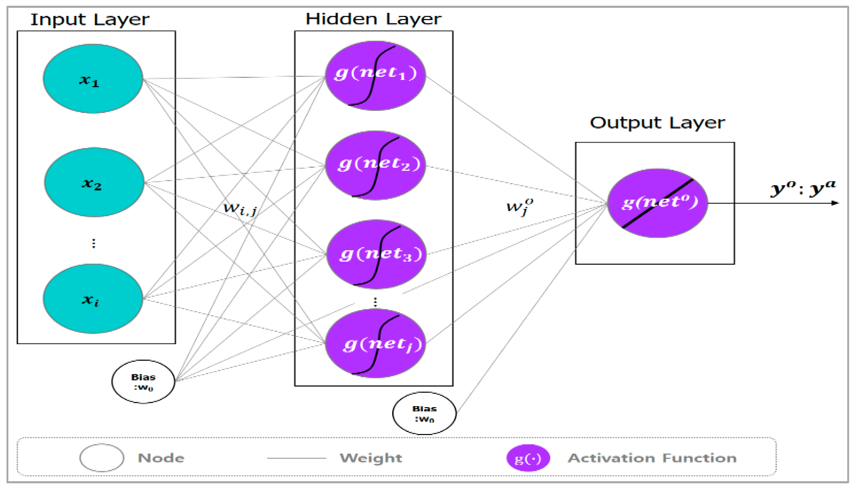
where $\eta$ denotes the learning rate constant and $\delta$ denotes the product of the error with the derivative of the transfer function. The number of hidden layers is a factor that significantly affects the prediction performance. According to a study by Cybenko [35] and Zhang et al. [36], sufficient prediction performance can be achieved even with one hidden layer to use one number. Figure 3 shows the schematic of the related ANN structure.

Machine learning models, such as ANNs, are useful in market forecasting; however, they are not without drawbacks. In the machine learning models, “overfitting” frequently occurs in the learning process because of the high dependence of the learning algorithm on given data, and sometimes the model has insufficient data size. Therefore, model-fitting must be carried out with careful interpretation of the set of data that is used. Particularly, important parameters that need to be determined are related to the number of required inputs, hidden layers, and hidden nodes. This is closely associated with optimal model selection. In order to successfully adjust the parameters, n-fold cross-validation techniques and grid search tools are applied. In addition, the raw data used in this paper was preprocessed by data scaling, called data normalization, which is crucial for improving the model’s performance. There are various scaling techniques used. Since there is no specific consensus or theories to decide on the best normalization technique [37,38,39], this paper used the min-max normalization technique $\left\{x-\min \left(x\right)\right\}/\{\max \left(x\right)-\min \left(x\right)\}$.

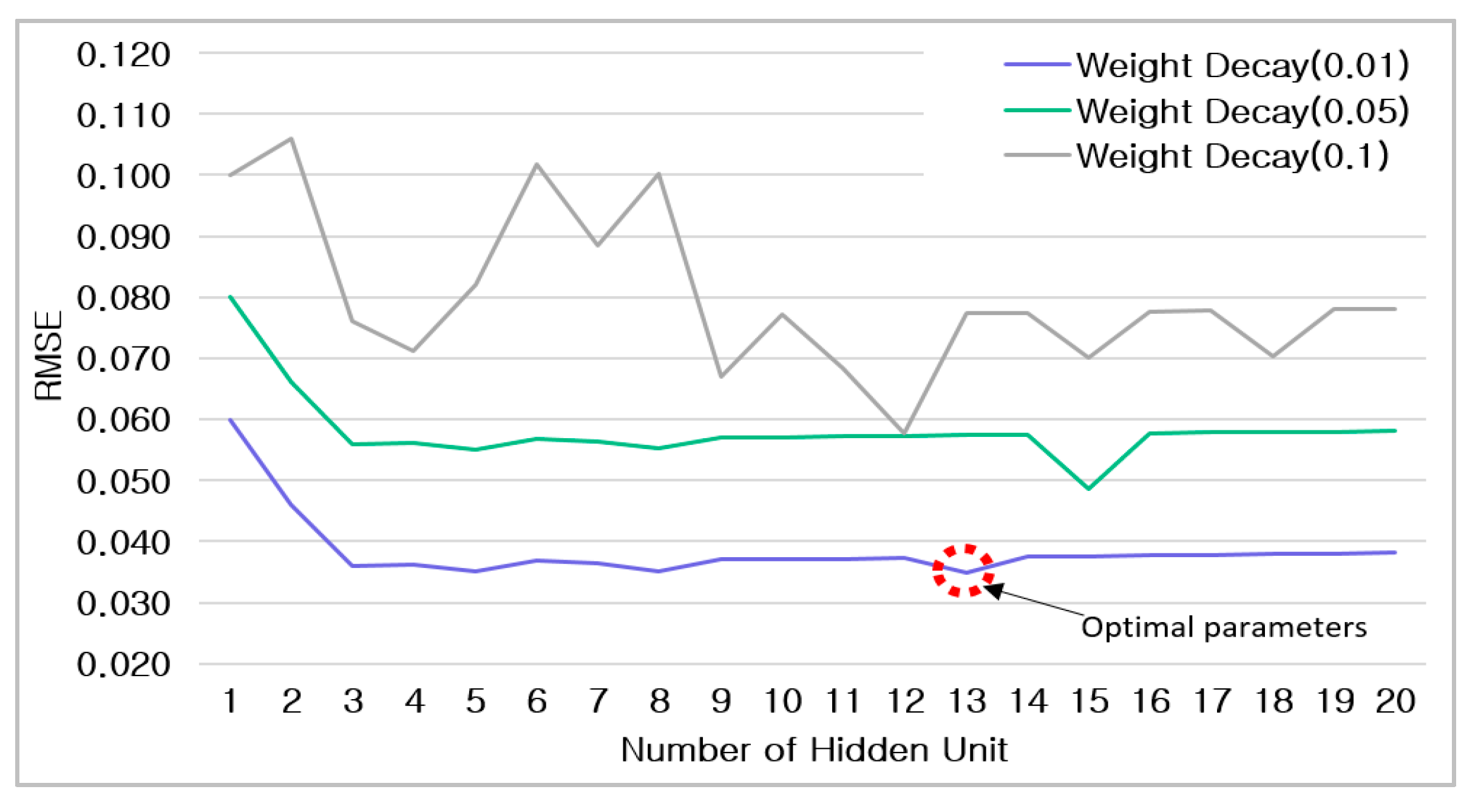
Subsequently, the data was divided into the train set and the test set in the ratio of 8:2, according to the literature. Then, the optimal parameters could be derived from the 10-fold cross-validation with the train set. As a result, the weight decay and the number of hidden neurons were 0.01 and 13, respectively, as shown in Figure 4. For the number of hidden layers, this paper used one layer because many previous studies proposed that their model worked well despite adopting a single layer [36,40,41,42].

2.2.3. Support Vector Regression Model

The SVM model can be divided into (1) support vector classification (SVC), which is applied to classification tasks, and (2) support vector regression (SVR), which tries to fit and deal with the optimal value through prediction. Considering the above-mentioned factors, this study used SVR. Vapnik [43] developed SVM, a model that finds the optimal hyperplane for data classification with linear and non-linear characteristics, devised “ε-insensitive SVR” through subsequent research data, and extended the model to the problem with prediction [44]. Unlike ANNs, which are commonly estimated via an empirical risk minimization structure, SVM with a structural risk minimization type is known for its superior generalization. Therefore, in the case of artificial neural networks, there is an underfitting or overfitting problem due to the local minima. The SVM is a supervised learning model, and is known for being free from the constraints of quadratic programming. The SVM can be expressed by Equation (5):

$$f\left(x\right)=w^T\varnothing \left(x_t\right)+b$$

(5)

where w is a weight vector, and ∅(x_t) is a mapping that transforms an input vector into a high-dimensional random feature space. Using the above equation, an optimization model that minimizes the objective function that imposes a penalty on the weight vector w can be constructed. Equation (6) is derived by applying the Lagrangian multiplier method to the objective function, expressed as a quadratic function:

$$f\left(x\right)={\displaystyle \sum }_{i=1}^n({\alpha }_i-{\alpha }_i^{\prime })K\left(x_i,x\right)+b$$

(6)

where ${\alpha }_i$ is the Lagrangian multiplier, and K(∙) is the kernel function. One of the biggest advantages of the SVM is that it uses a kernel function, which can solve the complexity of high-dimensional space calculations. Therefore, this study used the radial basis function network, as shown in Equation (7):

$$K\left(x_t,x\right)=\exp (\frac{-\left|\right|x-x_t\left|\right|{}^2}{2{\sigma }^2})$$

(7)

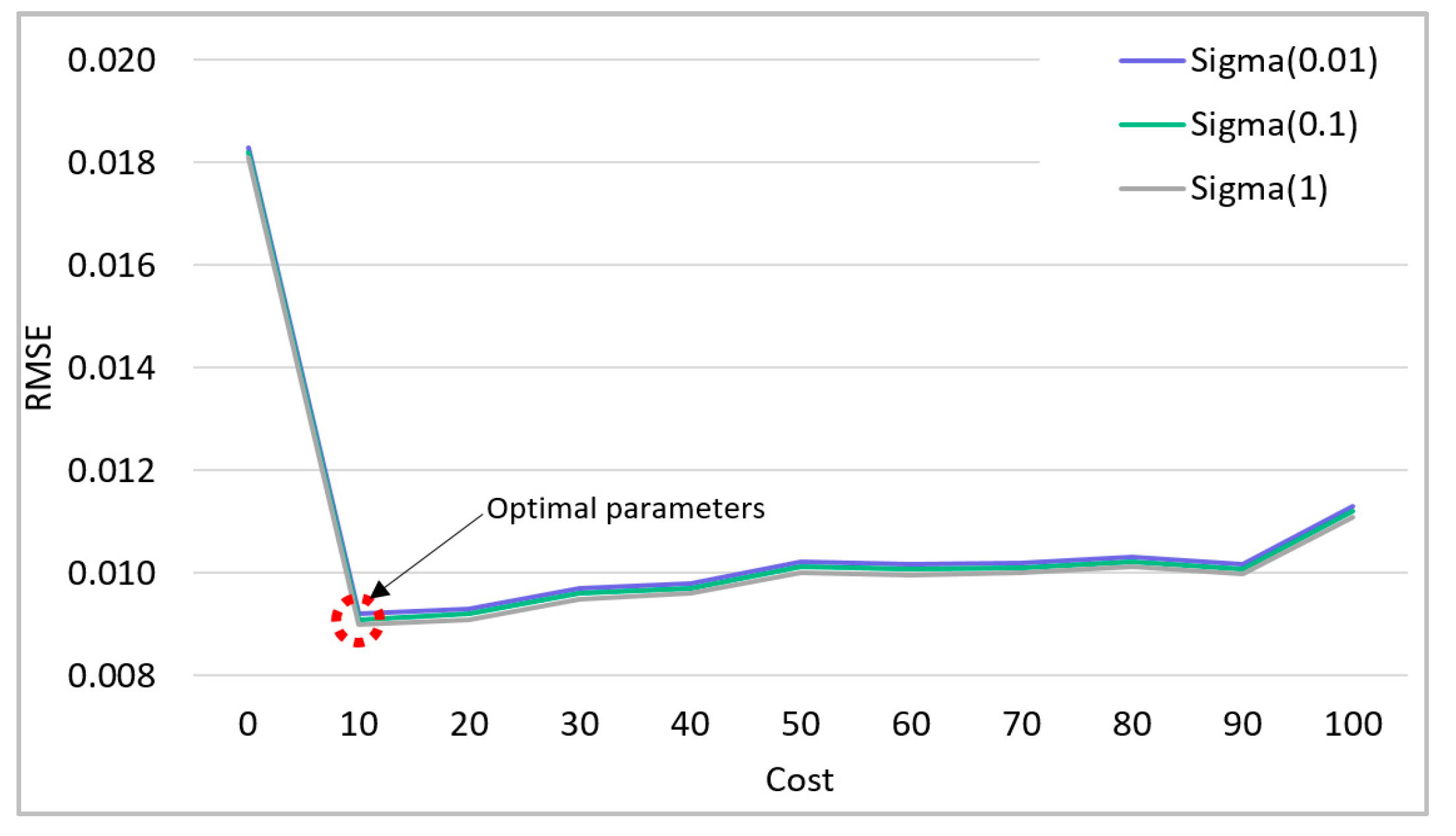
For SVR, the usage of kernel functions makes it a more powerful model than others. As mentioned before, unlike other models, SVR pursues the structural risk principle. Many researchers have pointed out that the main advantage of the SVR is its global optimality. However, the excellent performance of this model is highly dependent on the selection of the cost and sigma parameters, and the kernel function. The grid search algorithm is tuned such that the optimal parameters have the minimum error; moreover, the cost (C) and sigma are 1 and 10, respectively, as shown in Figure 5. There are various kernel functions, such as linear, polynomial, and sigmoid types. This study chose the radial basis kernel (called Gaussian) to set the model because it is a proven method, based on previous studies.

2.2.4. Random Forest Model

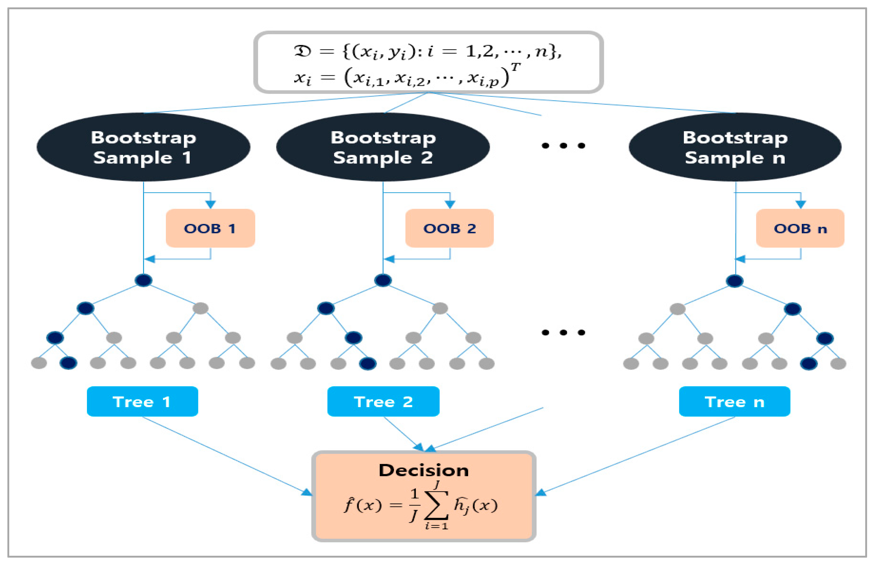
Breiman [45] proposed the random forest (RF) algorithm, which incorporates the concept of decision trees and bagging. This model can be applied from classification to regression; it is relatively fast to learn, its parameters can be tuned easily, it can be applied to high-dimensional problems, and it can be easily implemented in parallel [46]. RF is a tree-based ensemble method, with each decision tree having a collection of random variables. The detailed algorithm for random forest is shown in Figure 6.

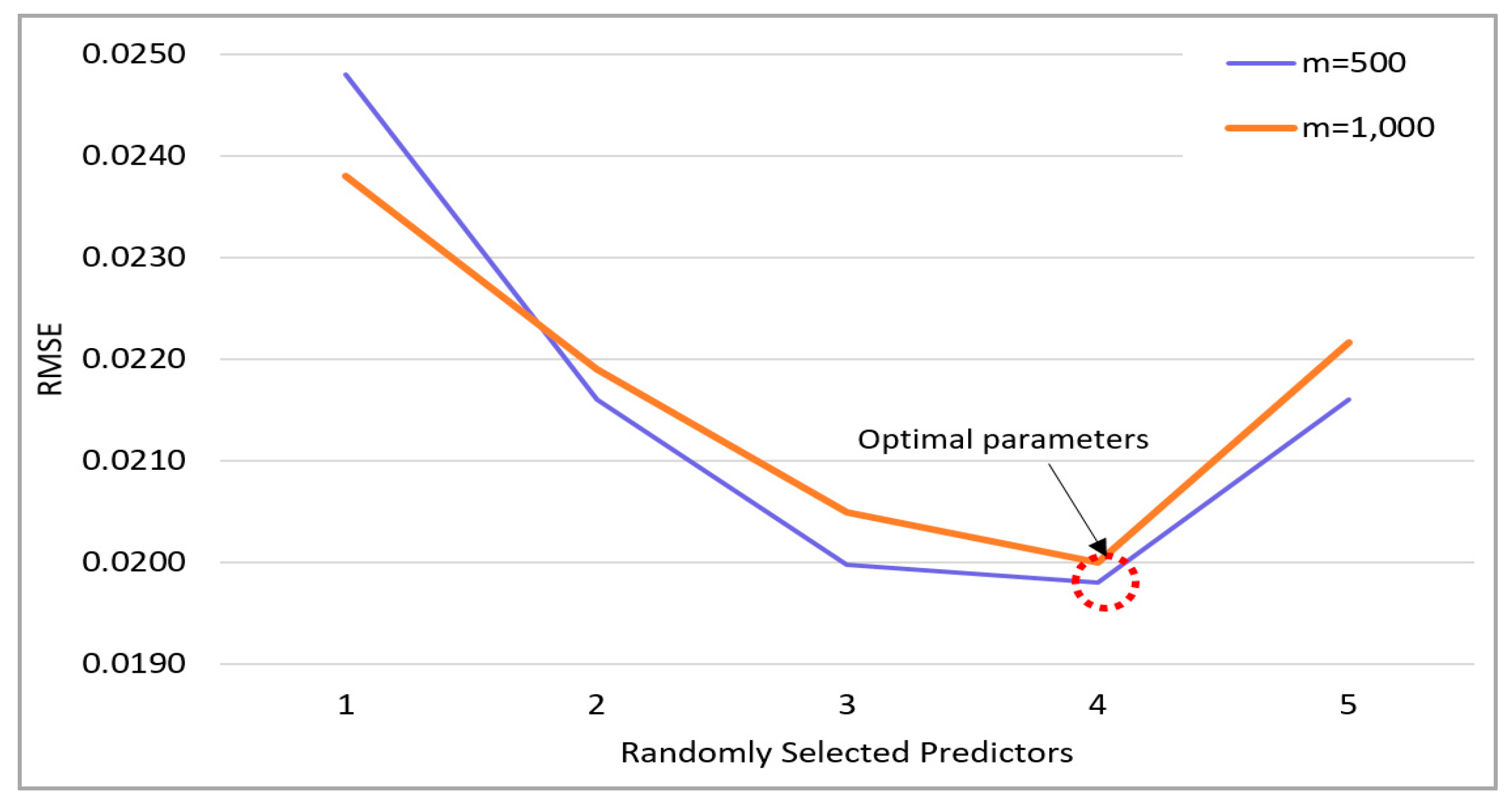
The RF model is the machine learning model derived from the decision tree, which can be used for both classification and regression problems. Since this tree-based model is prone to overfitting, treating the overfitting phenomenon is crucial to improving its performance. Generally, the stopping rule or the pruning technique is adopted to regularize the RF model. Breiman [45] devised the bootstrapped trees called out-of-bag (OOB) in the learning process, which is similar to the bagging of the decision tree. These bootstrapped trees with randomly selected m predictors among all the p predictors are statistically uncorrelated to each other. Typically, this m is known as an approximation of $\sqrt{p}$. The m parameter is presented in Figure 7 through cross-validation, and the OOB is 500 random trees.

The optimal parameter values of each model were found through the above experiments; they can be summarized as shown in

Table 4. Summary of optimal parameters for each machine learning model.

Model	Parameters
ANN	Number of Hidden Nodes	Weight Decay
	13	0.01
SVR	Cost	Sigma
	10	1
RF	Number of m Predictors	Number of Trees
	4	500

. This paper evaluated the economic value of the T/C extension option based on the briefly introduced methods and their optimal parameters thus far. Finally, the proper valuation model is proposed by comparing various candidate models with the BSM, ANN, SVR, and RF.

3. Empirical Results and Discussion

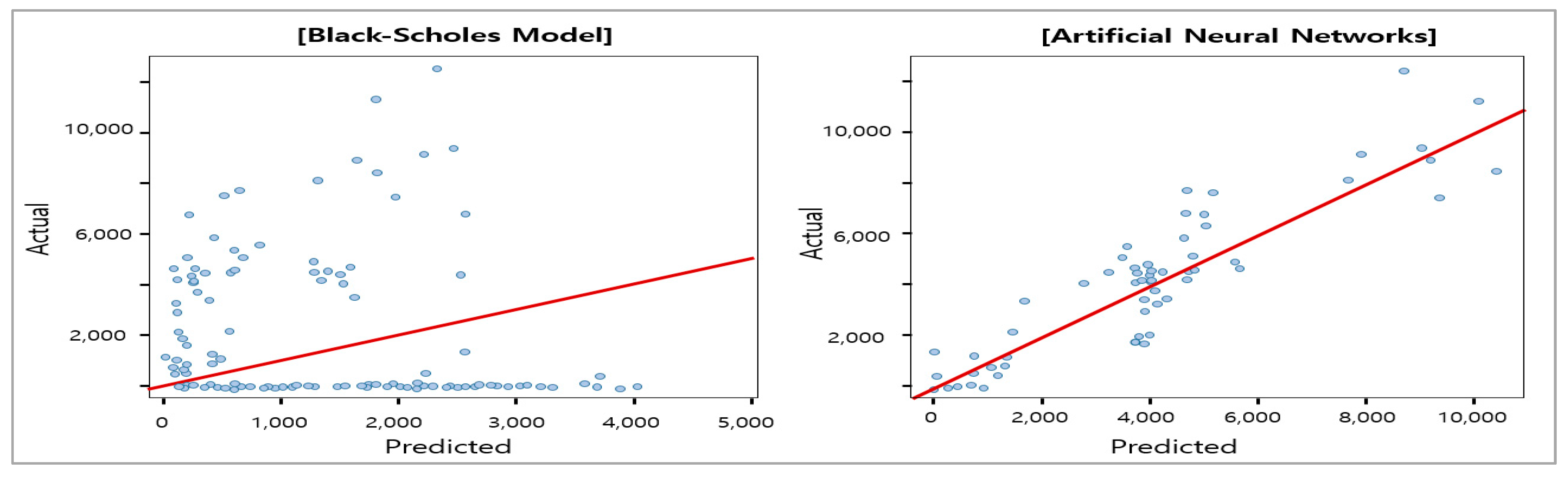
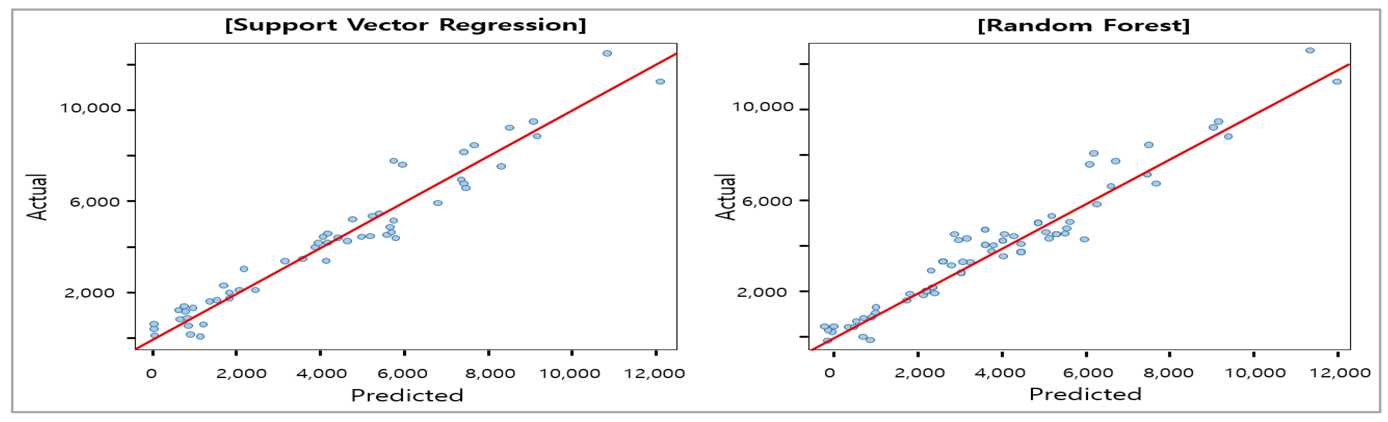
Given the optimal parameters and the test sample, each proposed model estimated the economic value of the T/C extension option. The comparisons between the actual value and predicted value of the option are depicted in Figure 8 and Figure 9. As illustrated in these figures, the performance of ML models such as ANN, SVR, and RF, were found to significantly outweigh the result of the BSM.

This paper evaluated the performance of the proposed models based on three criteria: the mean absolute error (MAE, $\frac{1}{n}{\displaystyle \sum }_{i=1}^n|y_i-{\widehat{y}}_i|$), the root mean square error (RMSE, $\sqrt{\frac{1}{n}{\displaystyle \sum }_{i=1}^n{(y_i-{\widehat{y}}_i)}^2}$), and the correlation coefficient (Cor, $\frac{Cov\left(y,\widehat{y}\right)}{{\sigma }_y{\sigma }_{\widehat{y}}}$), where $\widehat{y}$ is the forecast, $y$ is the actual observation, $\mathrm{Cov}()$ is the covariance, and $\sigma$ is the standard deviation. The MAE and RMSE have scale-dependent criteria. The alternative measure is the correlation coefficient, showing the linearity between the actual value and the forecast. The lower the numerical value of the MAE and RMSE, the better the performance is. For the correlation coefficient, values closer to 1 indicate better performance. The measures of the performances are summarized in

Table 5. Summary of option pricing.

Measures	BSM	ANN	SVR	RF
MAE	2141.2	364.7	217.9	165.5
RMSE	2848.6	684.9	468.1	401.8
Cor	0.004	0.912	0.947	0.951

Note: MAE is mean absolute error, RMSE is the root mean square error, Cor is the correlation coefficient.

. Compared to the benchmark model BSM, all of the ML models exhibited fair performance. More precisely, the RF showed the best result of the most precise value of the T/C extension option that could be taken, which is provided to charterers at no cost in the LNG market.

As confirmed in Table 5, compared to the machine learning model, the performance level of the conventional model is significantly poor. The BSM is well suited for the valuations of derivatives in financial markets, such as securities, commodities, and others, and it has been recognized for its performance. The disappointing result of the BSM here is due to the inability of the model to capture the extreme volatility of the shipping freight rate; moreover, this model requires normally distributed data, which is not the actual state of the available data. In other words, these data are more appropriate to machine learning models that do not require presumptions of the data and the model. The best model concerning the resultant performances are in the order of RF, SVR, ANN, and BSM.

In terms of model performance, the RF model’s good ability to price the economic value of the option is quite meaningful, because the RF model is more intuitive than the ANN and SVR. This feature is based on the parallel establishment of simple decision trees, and the model can identify the number of important variables and their significances rapidly [42,45,46,47]. That is, the RF model is easily acceptable, interpretable, and practicable in shipping fields.

From a practical perspective, this paper presents the possibility of pricing the economic value of the T/C extension option in the LNG freight market. Since this option is generally granted to charterers with high credibility at no cost to make the contract more appealing, this value can be used for the latent credibility of the contract counterpart. Therefore, this value of the option can be the proxy of the charterers’ credit. In addition, if the ship owner has numerous T/C extension options, shipping investors consider that the size of the option may impose financial burdens on the shipping companies, or may undermine the companies’ values. In other words, if the charterers hold sizable options, they can increase the value of their financial assets.

In summary, the valuation of the extension option to extend the period of the LNG freight contract is valuable for the decision making of LNG shipping market players, in terms of their corporate value. Eventually, the valuation of the T/C extension option should be necessary for the efficiency of the LNG freight market.

4. Conclusions

This study estimated the value of the T/C extension option in the LNG freight contract, which is provided by ship owners to charterers at no cost in common shipping practices. This extension clause in the contract grants the charterer the opportunity to take advantage of the option to extend the period of the original T/C contract at the same rate as the original rate when expired. Unlike general derivatives, which are tradeable and come with a risk premium, the T/C extension option is not tradeable and is conventionally provided free of charge. Although options have considerable economic value, the two parties to the contracts have been using them without evaluation. Since these options can be recognized as companies’ assets or liabilities, they should be evaluated. This paper is expected to provide the LNG shipping industry with prominent valuation methods in order to assess the fair value of the T/C extension option.

Although the benchmark model, the BSM, is eminent in financial markets, its logic is not appropriate for the valuation of derivatives in the shipping freight market. The candidates proposed in this paper were machine learning models such as the ANN, SVR, and the RF model. In the empirical experiment, their performances were significantly superior to the benchmark model. The reason why the machine learning models significantly outweighed the BSM is that they do not require presumption of the data condition and the modeling process. Specifically, the results of the RF model best approximated the actual value of the T/C extension option. These results are highly promising in real shipping practices, because the RF model is more competitive than other models in terms of time consumption, complexity, accuracy, and interpretation. For these reasons, the RF model can be easily accepted practically without resistance.

Thus far, this study showed that machine learning models can be the valuation models of the period extension option embedded in the LNG time charter party. Since they perform better in the option valuation in shipping chartering practices, they are expected to become good alternatives. This paper presented the possibilities of applying machine learning models in the valuation of shipping derivatives. Furthermore, the implication of these possibilities is significant in the LNG shipping market, because it will trigger additional studies in the LNG trading business.

While this paper may convey a new intuition and models in academia and in fields related to LNG freight, there are still some limitations. Firstly, this paper used only the LNG 160,000 m³ freight rate to evaluate machine learning-based valuation models, because of data availability. There are also 145,000 m³ and 174,000 m³ rates, but their freight markets have not been tracked sufficiently long since data series were published. In order to generalize the results of the proposed models, further assessments are needed when their markets are sufficiently mature. Secondly, this paper did not adjust modeling details, such as the number of hidden layers, types of activation functions, and normalization methods, because this paper focused on the applicability of machine learning models in the valuation of the T/C extension option, which has not been previously studied. In order to obtain better performance of the models, machine learning modeling should further include the adjustment process in terms of the above factors, under more sophisticated techniques. In the near future, further research will be carried out to address these limitations.

References

- Hartley, P.R. The Future of Long-Term LNG Contracts. Energy J. 2015, 36, 209–233, Published by: International Association for Energy Economics. Available online: https://www.jstor.org/stable/24696008 (accessed on 20 July 2022). [CrossRef]
- Global LNG Market Outlook 2021. Available online: https://ihsmarkit.com/topic/global-lng-market-outlook-2021.html (accessed on 1 April 2022).
- Spot and Short-Term LNG Volumes in Total Trade. Available online: https://www.iea.org/data-and-statistics/charts/spot-and-short-term-lng-volumes-in-total-trade-2015-2020 (accessed on 4 April 2022).
- Baker, A.; Kenny, J.; Kimball, J.; Belknap, T.H., Jr. Time Charters; Routledge: London, UK, 2014. [Google Scholar]
- LNGVOY. Available online: https://www.bimco.org/contracts-and-clauses/bimco-contracts/lngvoy (accessed on 4 April 2022).
- LNG Charteringan Introduction. Available online: https://www.lexisnexis.co.uk/legal/guidance/lng-chartering-an-introduction (accessed on 8 April 2022).
- Alizadeh, A.H.; Nomikos, N.K. Freight Derivatives and Risk Management in Shipping, 2nd ed.; Palgrave Macmillan: London, UK, 2009. [Google Scholar]
- Yun, H.; Lim, S.; Lee, K. The value of options for time charterparty extension: An artificial neural networks (ANN) approach. Marit. Policy Manag. 2018, 45, 197–210. [Google Scholar] [CrossRef]
- Raju, T.B.; Sengar, V.S.; Jayaraj, R.; Kulshrestha, N. Study of Volatility of New Ship Building Prices in LNG Shipping. e-Navi 2016, 5, 61–73. [Google Scholar] [CrossRef]
- Lim, K.G.; Lim, M. Financial performance of shipping firms that increase LNG carriers and the support of eco-innovation. J. Shipp. Trade 2020, 5, 23. [Google Scholar] [CrossRef]
- Maritime Forecast to 2050—Enegy Transition Outlook 2018. DNV-GL. Available online: https://www.dnv.com/maritime/publications (accessed on 2 April 2022).
- Li, J.; Parsons, M.G. Forecasting tanker freight rate using neural networks. Marit. Policy Manag. 1997, 24, 9–30. [Google Scholar] [CrossRef]
- Mostafa, M.M. Forecasting the Suez Canal Traffic: A Neural Network Analysis. Marit. Policy Manag. 2004, 31, 139–156. [Google Scholar] [CrossRef]
- Yang, H.; Dong, F.; Ogandaga, M. Forewarning of Freight Rate in Shipping Market Based on Support Vector Machine. In Traffic and Transportation Studies; Mao, B., Tian, Z., Huang, H., Gao, Z., Eds.; ASCE: Nanning, China, 2008; pp. 295–303. [Google Scholar] [CrossRef]
- Fan, S.; Ji, T.; Gordon, W.; Rickard, B. Forecasting Baltic Dirty Tanker Index by Applying Wavelet Neural Networks. J. Transp. Technol. 2013, 3, 68–87. [Google Scholar] [CrossRef][Green Version]
- Lyridis, D.; Zacharioudakis, P.; Iordanis, S.; Daleziou, S. Freight-Forward Agreement Time series Modelling Based on Artificial Neural Network Models. Stroj. Vestn. J. Mech. Eng. 2013, 59, 511–516. [Google Scholar] [CrossRef]
- Santos, A.A.P.; Junkes, L.N.; Pires, F.C.M., Jr. Forecasting period charter rates of VLCC tankers through neural networks: A comparison of alternative approaches. Marit. Econ. Logist. 2014, 16, 72–91. [Google Scholar] [CrossRef]
- Han, Q.; Yan, B.; Ning, G.; Yu, B. Forecasting dry bulk freight index with improved SVM. Math. Probl. Eng. 2014, 2014, 460684. [Google Scholar] [CrossRef]
- Daranda, A. Neural Network Approach to Predict Marine Traffic. Balt. J. Mod. Comput. 2016, 4, 483–495. Available online: https://www.bjmc.lu.lv/fileadmin/user_upload/lu_portal/projekti/bjmc/Contents/4_3_8_Daranda.pdf (accessed on 10 May 2022).
- Bao, J.; Pan, L.; Xie, Y. A new BDI forecasting model based on support vector machine. In Proceedings of the 2016 IEEE Information Technology, Networking, Electronic and Automation Control Conference, Chongqing, China, 20–22 May 2016; pp. 65–69. [Google Scholar] [CrossRef]
- Shipping Intelligence Network. Available online: https://sin.clarksons.net (accessed on 31 May 2022).
- Black, F.; Scholes, M. The Pricing of Options and Corporate Liabilities. J. Polit. Econ. 1973, 81, 637–654. [Google Scholar] [CrossRef]
- Merton, R.C. Theory of rational option pricing. Bell J. Econ. Manag. Sci. 1973, 4, 141–183. [Google Scholar] [CrossRef]
- Hull, J.C. Options Futures and Other Derivatives, 11th ed.; Pearson: Hoboken, NJ, USA, 2022. [Google Scholar]
- Lajbcygier, P.R.; Conner, J.T. Improved option pricing using artificial neural networks and bootstrap methods. Int. J. Neural Syst. 1997, 8, 457–471. [Google Scholar] [CrossRef]
- Andreou, P.C.; Charalambous, C.; Martzoukos, S.H. Robust Artificial Neural Networks for Pricing of European Options. Comput. Econ. 2006, 27, 329–351. [Google Scholar] [CrossRef]
- Shinde, A.S.; Takale, K.C. Study of Black-Scholes model and its applications. Procedia Eng. 2012, 38, 270–279. [Google Scholar] [CrossRef]
- Liu, S.; Oosterlee, C.W.; Bohte, S.M. Pricing Options and Computing Implied Volatilities using Neural Networks. Risks 2019, 7, 16. [Google Scholar] [CrossRef]
- Smith, K.A.; Gupta, J.N.D. Neural networks in business: Techniques and applications for the operations researcher. Comput. Oper. Res. 2000, 27, 1023–1044. [Google Scholar] [CrossRef]
- Zhang, G.P. Time series forecasting using a hybrid ARIMA and neural network model. Neurocomputing 2003, 50, 159–175. [Google Scholar] [CrossRef]
- Roh, T.H. Forecasting the volatility of stock price index. Expert Syst. Appl. 2007, 33, 916–922. [Google Scholar] [CrossRef]
- Kristjanpoller, W.; Minutolo, M.C. Gold price volatility: A forecasting approach using the Artificial Neural Network-GARCH model. Expert Syst. Appl. 2015, 42, 7245–7251. [Google Scholar] [CrossRef]
- Kaastra, I.; Boyd, M. Designing a neural network for forecasting financial and economic time series. Neurocomputing 1996, 10, 215–236. [Google Scholar] [CrossRef]
- Tkáč, M.; Verner, R. Artificial neural networks in business: Two decades of research. Appl. Soft Comput. 2016, 38, 788–804. [Google Scholar] [CrossRef]
- Cybenko, G. Approximation by superpositions of a sigmoidal function. Math. Control Signals Syst. 1989, 2, 303–314. [Google Scholar] [CrossRef]
- Zhang, G.; Patuwo, E.B.; Michael, Y.H. Forecasting with artificial neural networks: The state of the art. Int. J. Forecast. 1998, 14, 35–62. [Google Scholar] [CrossRef]
- Ahsan, M.M.; Mahmud, M.A.P.; Saha, P.K.; Gupta, K.D.; Siddique, Z. Effect of Data Scaling Methods on Machine Learning Algorithms and Model Performance. Technologies 2021, 9, 52. [Google Scholar] [CrossRef]
- Ambarwari, A.; Adrian, Q.J.; Herdiyeni, Y. Analysis of the Effect of Data Scaling on the Performance of the Machine Learning Algorithm for Plant Identification. J. Resti (Rekayasa Sist. Dan Teknol. Inf.) 2020, 4, 117–122. [Google Scholar] [CrossRef]
- Shahriyari, L. Effect of normalization methods on the performance of supervised learning algorithms applied to HTSeq-PKMUQ data sets: 7SK RNA expression as a predictor of survival in patients with colon adenocarcinoma. Brief. Bioinf. 2019, 20, 985–994. [Google Scholar] [CrossRef]
- Basheer, I.A.; Hajmeer, M. Artificial neural networks: Fundamentals, computing, design, and application. J. Microbiol. Methods 2000, 43, 3–31. [Google Scholar] [CrossRef]
- Fadlalla, A.; Lin, C.H. An Analysis of the Applications of Neural Networks in Finance. Interfaces 2001, 31, 112–122. [Google Scholar] [CrossRef]
- Atsalakis, G.S.; Valavanis, K.P. Surveying stock market forecasting techniques—Part II: Soft computing methods. Expert Syst. Appl. 2009, 36, 5932–5941. [Google Scholar] [CrossRef]
- Vapnik, V.N. The Nature of Statistical Learning Theory; Springer: New York, NY, USA, 1995. [Google Scholar] [CrossRef]
- Vapnik, V.N. Statistical Learning Theory; Wiley: New York, NY, USA, 1997. [Google Scholar] [CrossRef]
- Breiman, L. Random Forests. Mach. Learn. 2001, 45, 5–32. [Google Scholar] [CrossRef]
- Cutler, A.; Cutler, D.R.; Stevens, J.R. Random Forest. In Ensemble Machine Learning-Methods and Applications; Zhang, C., Ma, Y., Eds.; Springer: New York, NY, USA, 2012. [Google Scholar] [CrossRef]
- Nguyen, D.T.; Kasmarik, K.E.; Abbass, H.A. Towards Interpretable ANNs: An Exact Transformation to Multi-Class Multivariate Decision Trees. arXiv 2021, arXiv:2003.04675. [Google Scholar]