
Short-Term Wind Power Prediction Based on Data Decomposition and Combined Deep Neural Network


Abstract
:1. Introduction
2. Methodology
2.1. Variational Mode Decomposition
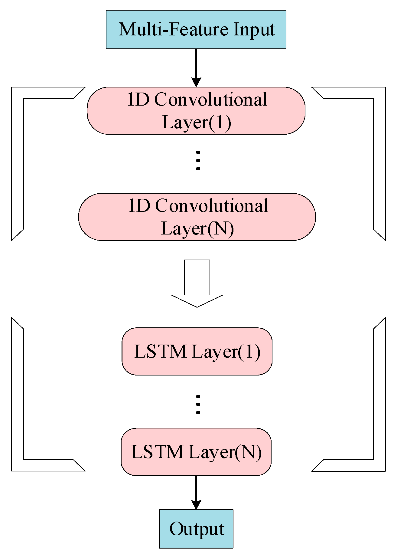
2.2. Convolutional Neural Network
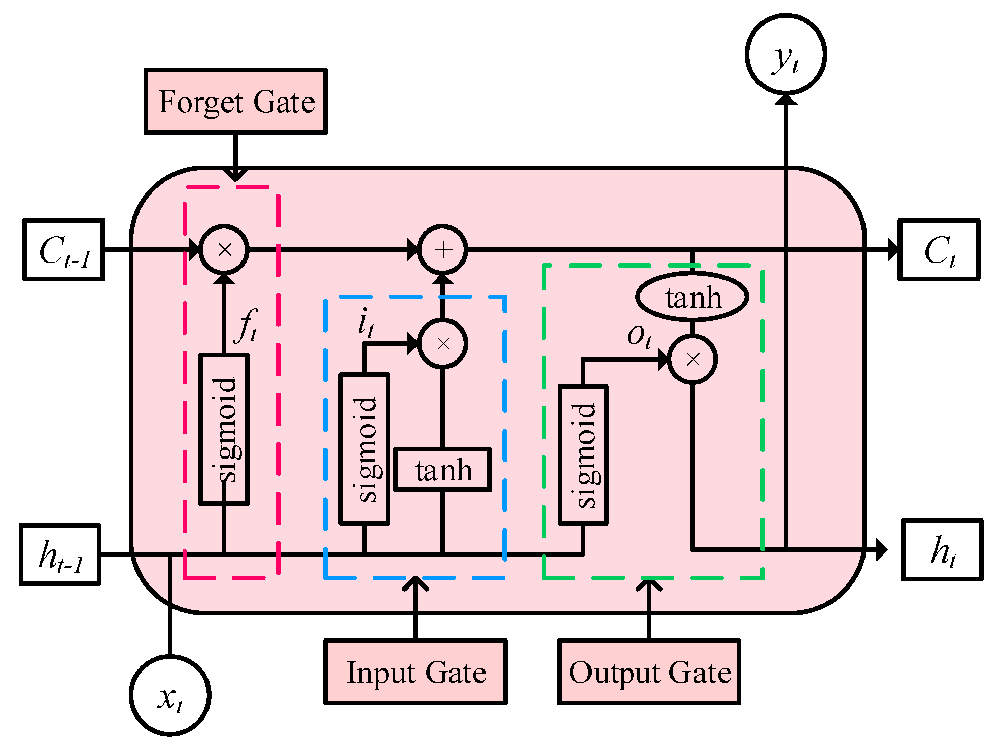
2.3. Long Short-Term Memory Neural Network
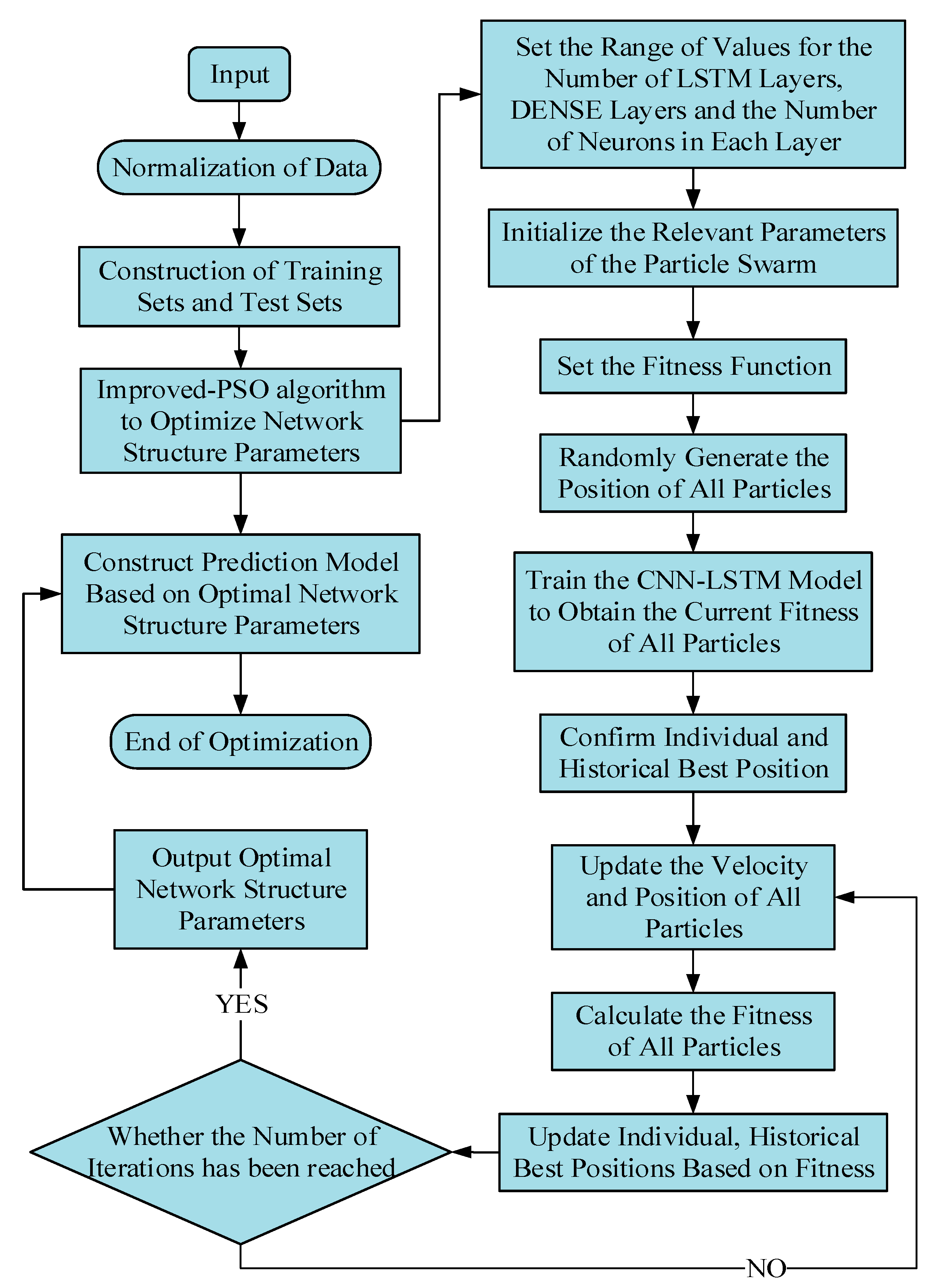
2.4. Adaptive Weighted Particle Swarm Algorithm Combined with Elimination Mechanism
3. Construction of Wind Power Prediction Model and Evaluation Metrics
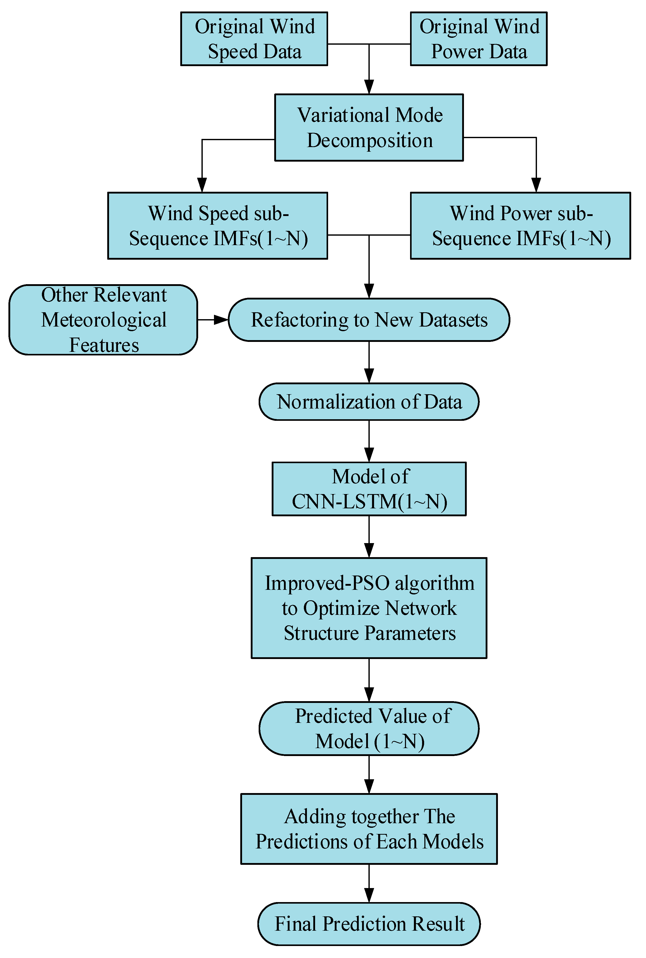
3.1. VMD-CNN-IPSO-LSTM Prediction Model
3.2. Evaluation Metrics
4. Case Study
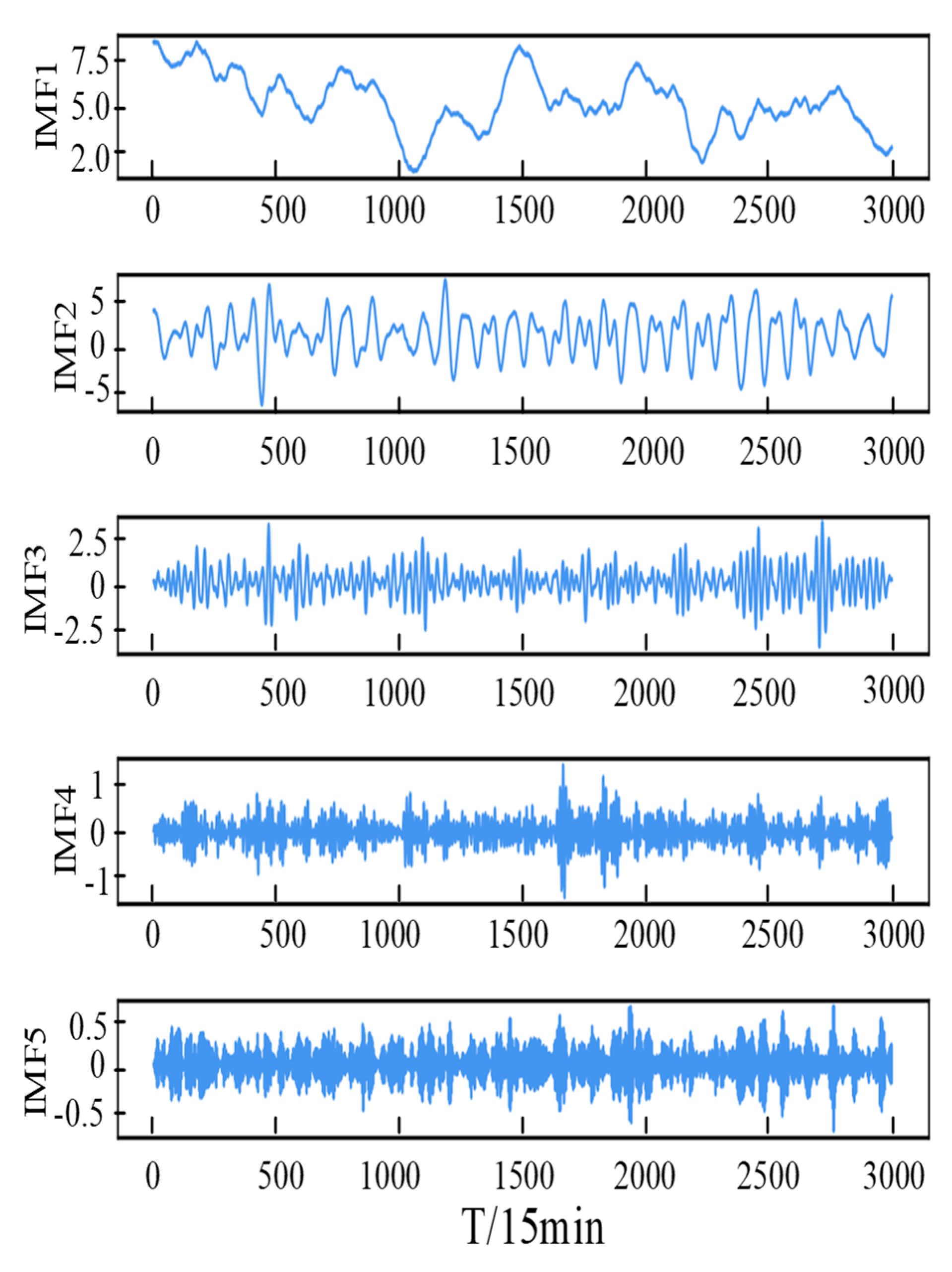
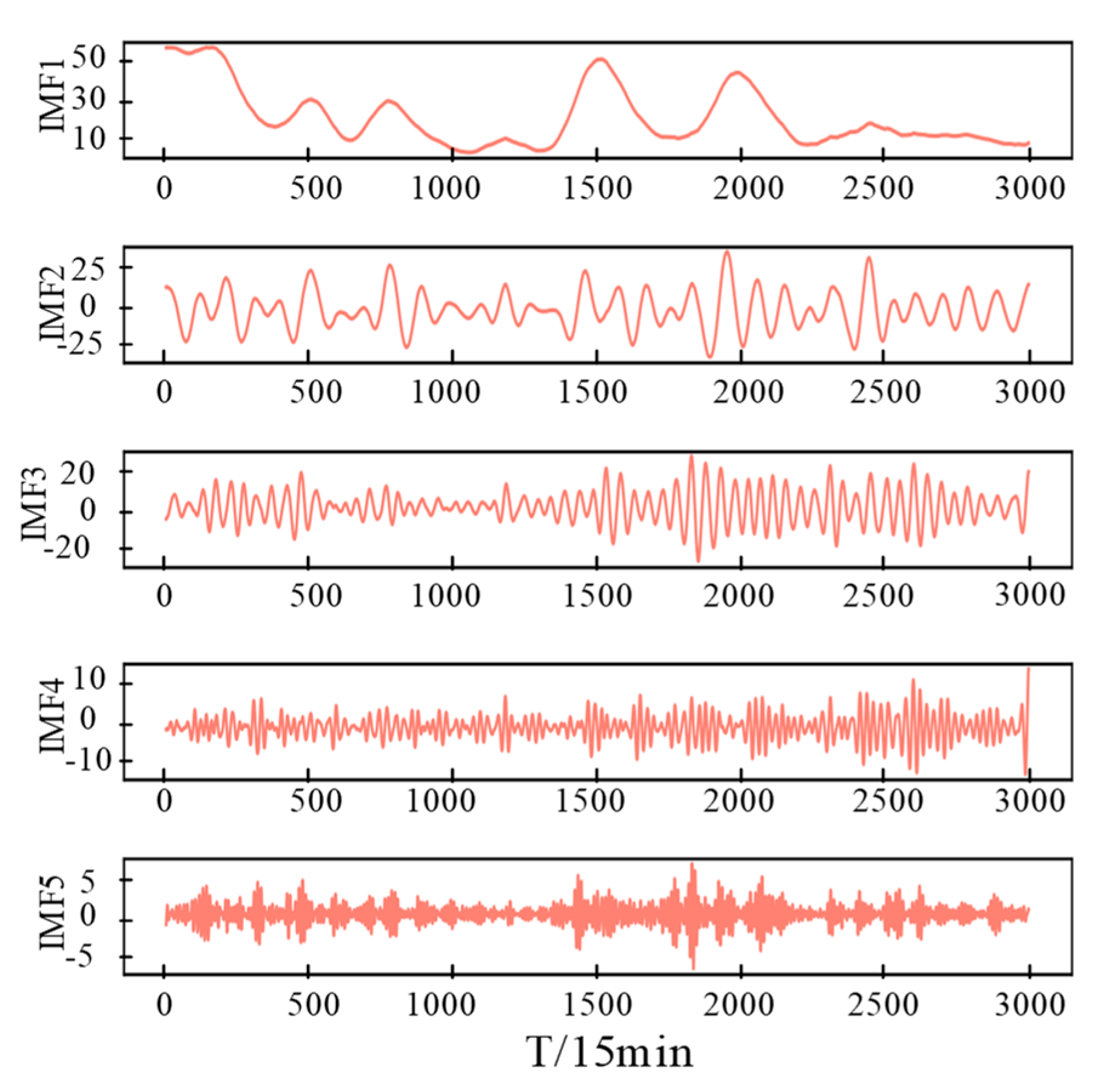
4.1. Decomposition of Wind Speed and Wind Power Series Using VMD
4.2. IPSO Optimized Prediction Model Network Structure Parameters
4.3. Verify the Generalization Ability of the Model under the New Data Set
5. Conclusions
- (1)
- The volatility and noise of wind speed and wind power series are effectively reduced after variational mode decomposition;
- (2)
- The combined deep neural network has a sharp learning ability for the data implicit feature. However, the overall consumption time is longer than that of the single model, so it is important to choose the number of decomposed modes reasonably. If the number of modes is too much or too little, it will have an impact on the hybrid model;
- (3)
- The network structure parameters of the prediction model can be optimized by the improved PSO algorithm to further enhance prediction accuracy;
- (4)
- To verify the generalized potential of the proposed model, the output of the same wind farm in two months with large climate difference is investigated. The analysis of the prediction results confirms that the model has a strong generalized ability;
- (5)
- For future research directions, the authors intend to use a multi-step decomposition model after which the sub-sequence obtained from the decomposition is passed through different neural networks for feature extraction, such as using graph convolutional neural networks for implicit mining, and to compare whether the model proposed in this paper makes a breakthrough in accuracy through simulation.
Author Contributions
Funding
Institutional Review Board Statement
Informed Consent Statement
Data Availability Statement
Conflicts of Interest
Abbreviations
| VMD | Variational Mode Decomposition |
| EMD | Empirical Mode Decomposition |
| CNN | Convolutional Neural Network |
| RNN | Recurrent Neural Network |
| LSTM | Long and Short-term Memory Neural Network |
| IPSO | Improved Particle Swarm Optimization |
| MAE | Mean Absolute Error |
| RMSE | Root Mean Square Error |
| MAPE | Mean Absolute Percentage Error |
| R2 | Coefficient of Determination |
| Adj-R2 | Adjusted R-Square |
| Output, Weight, Threshold of the ith Convolution Kernel in the kth Layer | |
| f | Activation Function |
| N | the Number of Input Convolution Kernels |
| Convolution Operation | |
| ft, it, ot | Outputs of the 3 Gates of LSTM |
| Wf, Wi, Wc, Wo | Weight matrix of LSTM |
| bf, bi, bc, bo | Biased vector of LSTM |
| , | Updated, Current Velocity of the ith Particle |
| , | Updated, Current Position of the ith Particle |
| w | Inertia Weight |
| c1, c2 | Learning Factor |
| r1, r2 | Random Number between [0, 1] |
| n | the Total Amount of Data Set |
| p | Number of features in the dataset |
| , , | True value, Predicted value, the Average of True Value |
References
- Zhou, J.; Xu, X.; Huo, X.; Li, Y. Forecasting models for wind power using extreme-point symmetric mode decomposition and artificial neural networks. Sustainability 2019, 11, 650. [Google Scholar] [CrossRef]
- Wang, Y.; Wang, D.; Tang, Y. Clustered hybrid wind power prediction model based on ARMA, PSO-SVM, and clustering methods. IEEE Access 2020, 8, 17071–17079. [Google Scholar] [CrossRef]
- Han, Y.; Tong, X. Multi-step short-term wind power prediction based on three-level decomposition and improved grey wolf optimization. IEEE Access 2020, 8, 67124–67136. [Google Scholar] [CrossRef]
- Zhang, Y.; Han, J.; Pan, G.; Xu, Y.; Wang, F. A multi-stage predicting methodology based on data decomposition and error correction for ultra-short-term wind energy prediction. J. Clean. Prod. 2021, 292, 125981. [Google Scholar] [CrossRef]
- Bokde, N.; Feijóo, A.; Villanueva, D.; Kulat, K. A review on hybrid empirical mode decomposition models for wind speed and wind power prediction. Energies 2019, 12, 254. [Google Scholar] [CrossRef]
- Li, M.; Li, Y. Dispatch Planning of a Wide-Area Wind Power-Energy Storage Scheme Based on Ensemble Empirical Mode Decomposition Technique. IEEE Trans. Sustain. Energy 2020, 12, 1275–1288. [Google Scholar] [CrossRef]
- Zhu, A.; Zhao, Q.; Wang, X.; Zhou, L. Ultra-Short-Term Wind Power Combined Prediction Based on Complementary Ensemble Empirical Mode Decomposition, Whale Optimisation Algorithm, and Elman Network. Energies 2022, 15, 3055. [Google Scholar] [CrossRef]
- Liu, Z.; Hara, R.; Kita, H. 24 h-ahead wind speed forecasting using CEEMD-PE and ACO-GA-based deep learning neural network. J. Renew. Sustain. Energy 2021, 13, 046101. [Google Scholar] [CrossRef]
- Zhang, C.; Ding, M.; Wang, W.; Bi, R.; Miao, L.; Yu, H.; Liu, L. An improved ELM model based on CEEMD-LZC and manifold learning for short-term wind power prediction. IEEE Access 2019, 7, 121472–121481. [Google Scholar] [CrossRef]
- Chen, X.; Lai, C.S.; Ng, W.W.; Pan, K.; Lai, L.L.; Zhong, C. A stochastic sensitivity-based multi-objective optimization method for short-term wind speed interval prediction. Int. J. Mach. Learn. Cybern. 2021, 12, 2579–2590. [Google Scholar] [CrossRef]
- Zhang, D.; Peng, X.; Pan, K.; Liu, Y. A novel wind speed forecasting based on hybrid decomposition and online sequential outlier robust extreme learning machine. Energy Convers. Manag. 2019, 180, 338–357. [Google Scholar] [CrossRef]
- Safari, N.; Chung, C.; Price, G. Novel multi-step short-term wind power prediction framework based on chaotic time series analysis and singular spectrum analysis. IEEE Trans. Power Syst. 2017, 33, 590–601. [Google Scholar] [CrossRef]
- Dragomiretskiy, K.; Zosso, D. Variational mode decomposition. IEEE Trans. Signal Process. 2013, 62, 531–544. [Google Scholar] [CrossRef]
- Ali, M.; Khan, A.; Rehman, N.U. Hybrid multiscale wind speed forecasting based on variational mode decomposition. Int. Trans. Electr. Energy Syst. 2018, 28, e2466. [Google Scholar] [CrossRef]
- Yin, H.; Ou, Z.; Huang, S.; Meng, A. A cascaded deep learning wind power prediction approach based on a two-layer of mode decomposition. Energy 2019, 189, 116316. [Google Scholar] [CrossRef]
- Zhang, H.; Yue, D.; Dou, C.; Li, K.; Hancke, G.P. Two-step wind power prediction approach with improved complementary ensemble empirical mode decomposition and reinforcement learning. IEEE Syst. J. 2021, 16, 2545–2555. [Google Scholar] [CrossRef]
- Li, L.-L.; Chang, Y.-B.; Tseng, M.-L.; Liu, J.-Q.; Lim, M.K. Wind power prediction using a novel model on wavelet decomposition-support vector machines-improved atomic search algorithm. J. Clean. Prod. 2020, 270, 121817. [Google Scholar] [CrossRef]
- An, G.; Jiang, Z.; Cao, X.; Liang, Y.; Zhao, Y.; Li, Z.; Dong, W.; Sun, H. Short-term wind power prediction based on particle swarm optimization-extreme learning machine model combined with AdaBoost algorithm. IEEE Access 2021, 9, 94040–94052. [Google Scholar] [CrossRef]
- Jan, F.; Shah, I.; Ali, S. Short-Term Electricity Prices Forecasting Using Functional Time Series Analysis. Energies 2022, 15, 3423. [Google Scholar] [CrossRef]
- Jaseena, K.; Kovoor, B.C. Decomposition-based hybrid wind speed forecasting model using deep bidirectional LSTM networks. Energy Convers. Manag. 2021, 234, 113944. [Google Scholar] [CrossRef]
- Wang, Y.; Zou, R.; Liu, F.; Zhang, L.; Liu, Q. A review of wind speed and wind power forecasting with deep neural networks. Appl. Energy 2021, 304, 117766. [Google Scholar] [CrossRef]
- Rahmani, R.; Yusof, R.; Seyedmahmoudian, M.; Mekhilef, S. Hybrid technique of ant colony and particle swarm optimization for short term wind energy forecasting. J. Wind Eng. Ind. Aerodyn. 2013, 123, 163–170. [Google Scholar] [CrossRef]
- Wu, X.; Lai, C.S.; Bai, C.; Lai, L.L.; Zhang, Q.; Liu, B. Optimal kernel ELM and variational mode decomposition for probabilistic PV power prediction. Energies 2020, 13, 3592. [Google Scholar] [CrossRef]
- Bo, H.; Niu, X.; Wang, J. Wind speed forecasting system based on the variational mode decomposition strategy and immune selection multi-objective dragonfly optimization algorithm. IEEE Access 2019, 7, 178063–178081. [Google Scholar] [CrossRef]
- Ma, Z.; Chen, H.; Wang, J.; Yang, X.; Yan, R.; Jia, J.; Xu, W. Application of hybrid model based on double decomposition, error correction and deep learning in short-term wind speed prediction. Energy Convers. Manag. 2020, 205, 112345. [Google Scholar] [CrossRef]
- Shi, X.; Lei, X.; Huang, Q.; Huang, S.; Ren, K.; Hu, Y. Hourly day-ahead wind power prediction using the hybrid model of variational model decomposition and long short-term memory. Energies 2018, 11, 3227. [Google Scholar] [CrossRef]
- Naik, J.; Bisoi, R.; Dash, P. Prediction interval forecasting of wind speed and wind power using modes decomposition based low rank multi-kernel ridge regression. Renew. Energy 2018, 129, 357–383. [Google Scholar] [CrossRef]
- Li, C.; Tang, G.; Xue, X.; Saeed, A.; Hu, X. Short-term wind speed interval prediction based on ensemble GRU model. IEEE Trans. Sustain. Energy 2019, 11, 1370–1380. [Google Scholar] [CrossRef]
- Ju, Y.; Sun, G.; Chen, Q.; Zhang, M.; Zhu, H.; Rehman, M.U. A model combining convolutional neural network and LightGBM algorithm for ultra-short-term wind power forecasting. IEEE Access 2019, 7, 28309–28318. [Google Scholar] [CrossRef]
- Liu, Y.; Guan, L.; Hou, C.; Han, H.; Liu, Z.; Sun, Y.; Zheng, M. Wind power short-term prediction based on LSTM and discrete wavelet transform. Appl. Sci. 2019, 9, 1108. [Google Scholar] [CrossRef] [Green Version]
- Zhang, Y.; Sun, H.; Guo, Y. Wind power prediction based on PSO-SVR and grey combination model. IEEE Access 2019, 7, 136254–136267. [Google Scholar] [CrossRef]
- Liu, J.; Shi, Q.; Han, R.; Yang, J. A Hybrid GA–PSO–CNN Model for Ultra-Short-Term Wind Power Forecasting. Energies 2021, 14, 6500. [Google Scholar] [CrossRef]

| Decomposition Method | Merit | Demerit |
|---|---|---|
| EMD | 1. Adaptive: automatic generation of basis functions based on the data itself, adaptive filtering characteristics, adaptive multi-resolution 2. Completeness: the properties of the original series can be reproduced by superimposing the decomposed components | 1. Endpoint effect: there is no guarantee that the left and right endpoints of the signal are exactly the local poles 2. Mode mixing: the signals of different characteristic scales appear in one IMF component, and the other is that the signals of the same characteristic scales are dispersed into different IMF components |
| EEMD | White noise is added to the original signal before each decomposition to overcome the mode mixing in the EMD method | Due to the addition of noise, there is a possibility of inaccuracy in the reconstructed signal and noise cannot be ignored after reconstruction |
| CEEMD | The CEEMD effectively solves the problems of inaccurate reconstruction caused by noise pollution in the EEMD by adding positive and negative pairs of noise | Differences in the number of IMFs generated during decomposition lead to errors in decomposition |
| SSA | SSA can be applied to a wide range of time series without model restrictions | SSA does not have an explicit method to determine a threshold to distinguish the signal component from the noise component |
| VMD | VMD transforms signal decomposition into non-recursive, variational decomposition mode, which can effectively overcome the mode mixing phenomenon generated in EMD and has stronger noise robustness and weaker endpoint effect than EMD | Empirical knowledge is needed to adjust the choice of the K parameter in VMD |
| This Work | Anfeng Zhu, et al. [7] | Chao Zhang, et al. [9] | Hao Yin, et al. [15] | Rasoul Rahmani, et al. [22] | |
|---|---|---|---|---|---|
| Country | China | China | China | Spain | Iran |
| Research context | Presenting a hybrid model combined with VMD and CNN-LSTM for short-term wind power prediction | A combined prediction model is proposed which employs CEEMD as a wind speed decomposition method as well as an Elman neural network to learn the relationship between wind speed and wind power | Presenting a novel hybrid wind power short-term prediction model for wind power prediction that is combined with CEEMD-LZC, ALO, and ELM network | Presenting a hybrid wind power prediction approach by applying a cascaded deep learning model and a two-layer of mode decomposition method | Presenting a new hybrid swarm technique applied in forecasting the wind energy that makes the best advantage of mixing search ability of ACO and PSO |
| Prediction interval | 15 min | 15 min | 1 h | 1 h | 1 h |
| Model considered | VMD CNN LSTM IPSO | CEEMD WOA Elman | CEEMD LZC LLE ALO ELM | EMD VMD CNN LSTM | ACO PSO HAP |
| Findings | Optimizing the network structure parameters of CNN-LSTM model by improved PSO algorithm to improve the prediction accuracy of wind power | The combined prediction model utilizes CEEMD as a wind speed decomposition method to effectively solve the problem of reconstruction error and low efficiency of wind speed decomposition by EEMD | The hybrid model uses LZC to evaluate the complexity of each IMF after applying CEEMD to decompose the wind power and merges the IMFs according to the value of complexity, thus reducing the overall complexity of the model and improving the training efficiency | The original time series is decomposed by EMD and the sub-series that need to be decomposed in two steps are filtered out and further decomposed by VMD, while the implied relationship between wind speed, wind direction, and wind power are extracted by CNN | With the hybrid algorithm of ACO and PSO for the search of parameter values in the mathematical model, it can converge more quickly than the single ACO and PSO algorithm, and the accuracy of the model is also optimal |
| Drawback | Further validation of the generalization capability of this model by obtaining data from wind farms in other regions would strengthen the generalization ability of this model | The high number of IMFs in the CEEMD decomposition may lead to a higher complexity of the combined model | The LLE method proposed in this paper, as a novel data dimensionality reduction method, effectively reduces the dimensionality of the data. However, traditional dimensionality reduction methods are missing for comparison, such as PCA and other methods | The two-step decomposition results in a complex model and an increase in the time used for model training | The mathematical model consists of the S-curve and parabola, but it would be useful for the simulation to provide reasons why the model is composed of both of two curves and how much the effect can be improved compared to a single curve case |
| Model | Prediction Performance Analysis | |||
|---|---|---|---|---|
| MAE | RMSE | MAPE | adj-R2 | |
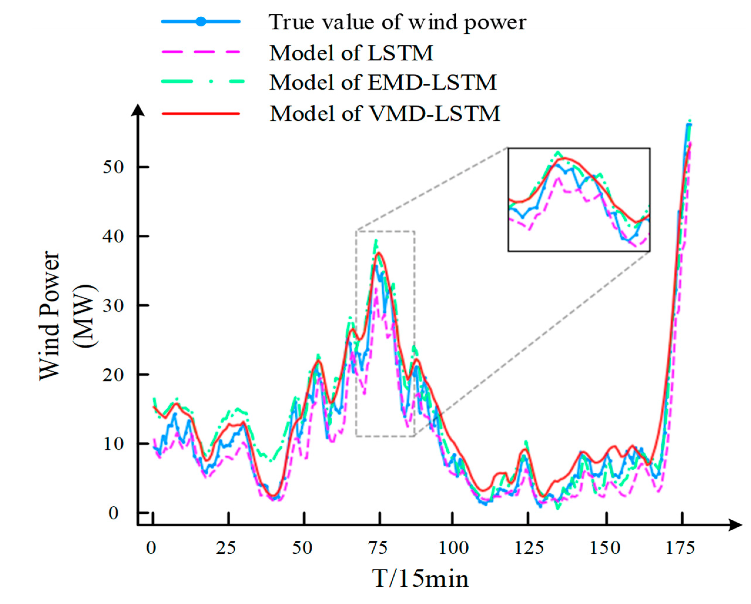
| LSTM | 2.38732 | 3.32454 | 0.59477 | 0.87264 |
| EMD-LSTM | 2.31746 | 2.88094 | 1.29272 | 0.90436 |
| VMD-LSTM | 2.14829 | 2.63109 | 1.46155 | 0.92023 |
| Combined Prediction Model | LSTM Layers | DENSE Layers | The Number of Neurons |
|---|---|---|---|
| Model 1 | 3 | 2 | 85/59/13/33/58 |
| Model 2 | 2 | 1 | 66/57/37 |
| Model 3 | 2 | 2 | 38/94/63/35 |
| Model 4 | 1 | 2 | 71/79/21 |
| Model 5 | 3 | 1 | 64/26/86/26 |
| Model | Prediction Performance Analysis | |||
|---|---|---|---|---|
| MAE | RMSE | MAPE | adj-R2 | |
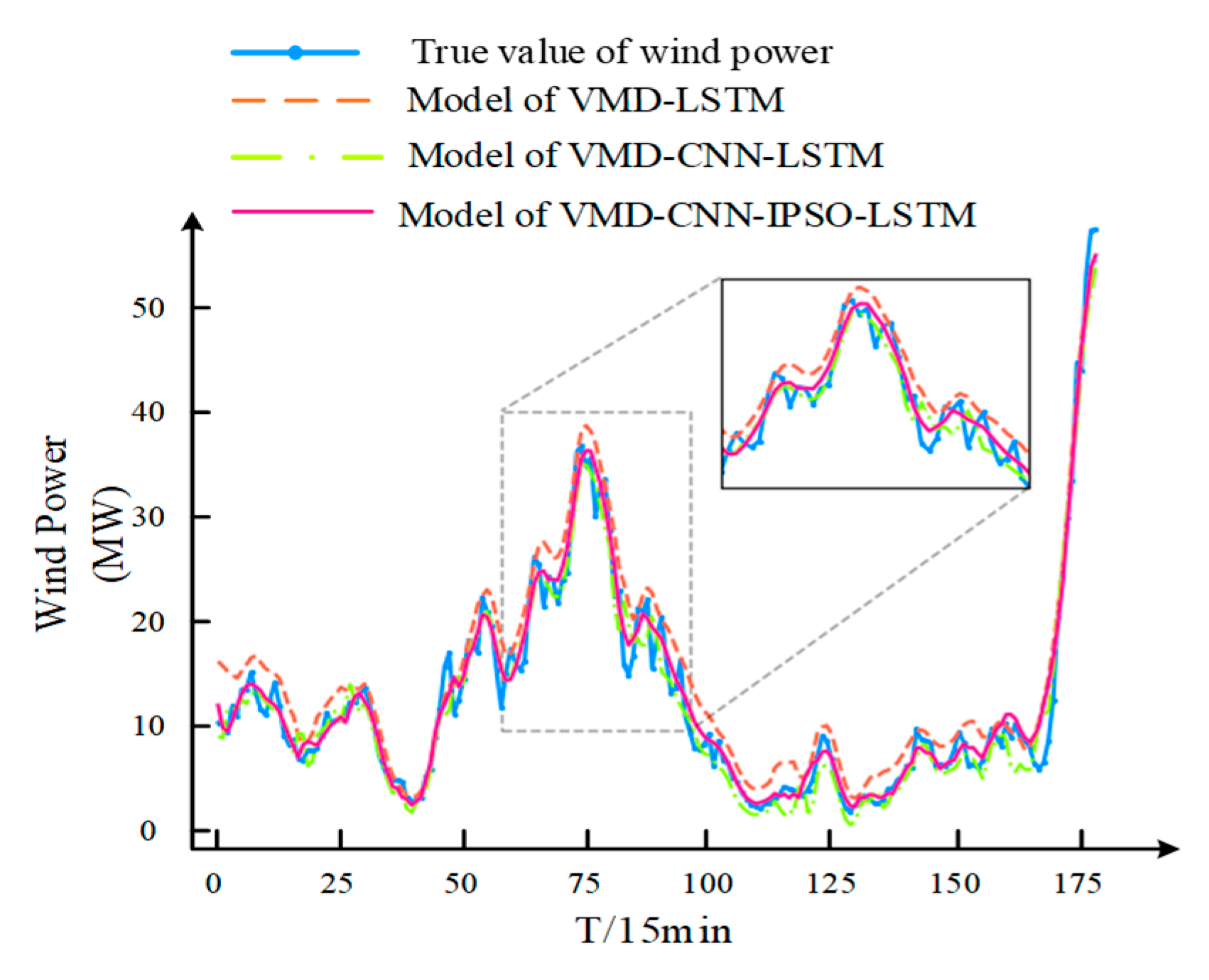
| VMD-LSTM | 2.14829 | 2.63109 | 1.46155 | 0.92023 |
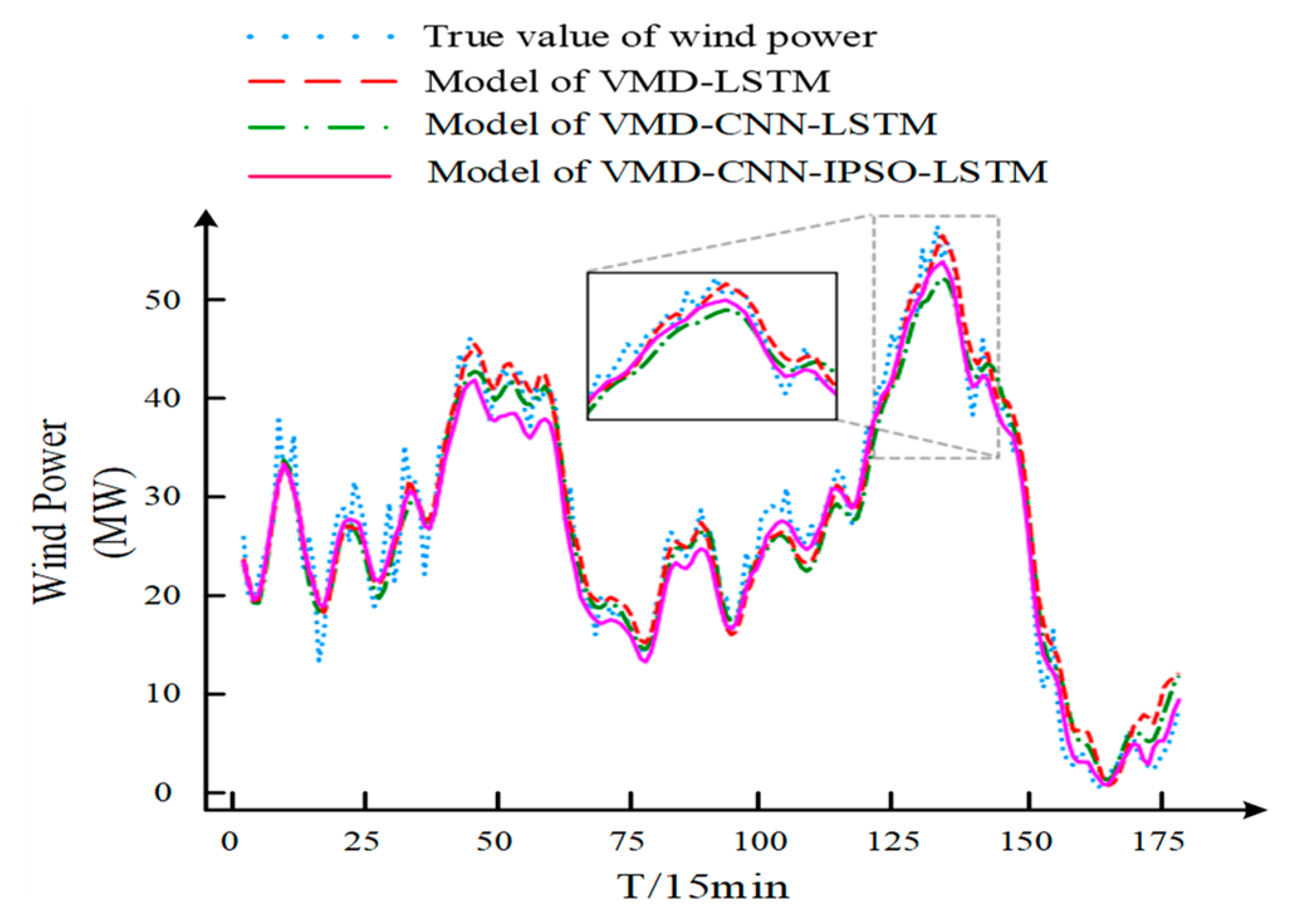
| VMD-CNN-LSTM | 1.48819 | 1.91680 | 1.38401 | 0.95766 |
| VMD-CNN-IPSO-LSTM | 1.10571 | 1.51672 | 0.43060 | 0.97349 |
| Combined Prediction Model | LSTM Layers | DENSE Layers | The Number of Neurons |
|---|---|---|---|
| Model 1 | 3 | 3 | 68/74/46/15/78/82 |
| Model 2 | 1 | 1 | 66/75 |
| Model 3 | 3 | 1 | 64/54/78/52 |
| Model 4 | 1 | 3 | 32/34/77/40 |
| Model 5 | 2 | 3 | 58/77/14/24/39 |
| Model | Prediction Performance Analysis | |||
|---|---|---|---|---|
| MAE | RMSE | MAPE | adj-R2 | |
| VMD-LSTM | 3.30657 | 4.07535 | 0.35427 | 0.95683 |
| VMD-CNN-LSTM | 3.20033 | 4.01825 | 0.43912 | 0.95803 |
| VMD-CNN-IPSO-LSTM | 2.92668 | 3.59604 | 0.20147 | 0.96639 |
Publisher’s Note: MDPI stays neutral with regard to jurisdictional claims in published maps and institutional affiliations. |
© 2022 by the authors. Licensee MDPI, Basel, Switzerland. This article is an open access article distributed under the terms and conditions of the Creative Commons Attribution (CC BY) license (https://creativecommons.org/licenses/by/4.0/).
Share and Cite
Wu, X.; Jiang, S.; Lai, C.S.; Zhao, Z.; Lai, L.L. Short-Term Wind Power Prediction Based on Data Decomposition and Combined Deep Neural Network. Energies 2022, 15, 6734. https://doi.org/10.3390/en15186734
Wu X, Jiang S, Lai CS, Zhao Z, Lai LL. Short-Term Wind Power Prediction Based on Data Decomposition and Combined Deep Neural Network. Energies. 2022; 15(18):6734. https://doi.org/10.3390/en15186734
Chicago/Turabian StyleWu, Xiaomei, Songjun Jiang, Chun Sing Lai, Zhuoli Zhao, and Loi Lei Lai. 2022. "Short-Term Wind Power Prediction Based on Data Decomposition and Combined Deep Neural Network" Energies 15, no. 18: 6734. https://doi.org/10.3390/en15186734
APA StyleWu, X., Jiang, S., Lai, C. S., Zhao, Z., & Lai, L. L. (2022). Short-Term Wind Power Prediction Based on Data Decomposition and Combined Deep Neural Network. Energies, 15(18), 6734. https://doi.org/10.3390/en15186734