
Optimal Allocation of Renewable Distributed Generators and Electric Vehicles in a Distribution System Using the Political Optimization Algorithm

 ,
, 
 ,
,  ,
,  , ,
, ,  and
and 
Abstract
:1. Introduction
- A combined approach such as VSI and POA is proposed to solve RDGs (Solar, Wind and Fuel cell) and EVCS allocation problems in DS. Furthermore, the uncertainties of RDGs, EV charging and discharging patterns are adequately considered.
- A voltage stability index (VSI) approach is utilized to decide the installation of DGs at weaker nodes and EVs at stronger nodes in the DS.
- This article determines the appropriate sizes of DGs (solar, wind and fuel cell) for specified load levels using a POA.
- The EVs are analysed while taking into account the essential aspects, along with the EV state of charge (SoC), travel constraints, EV battery size, and charging/discharging ranges. An optimized charging technique for charging and discharging EVs is offered.
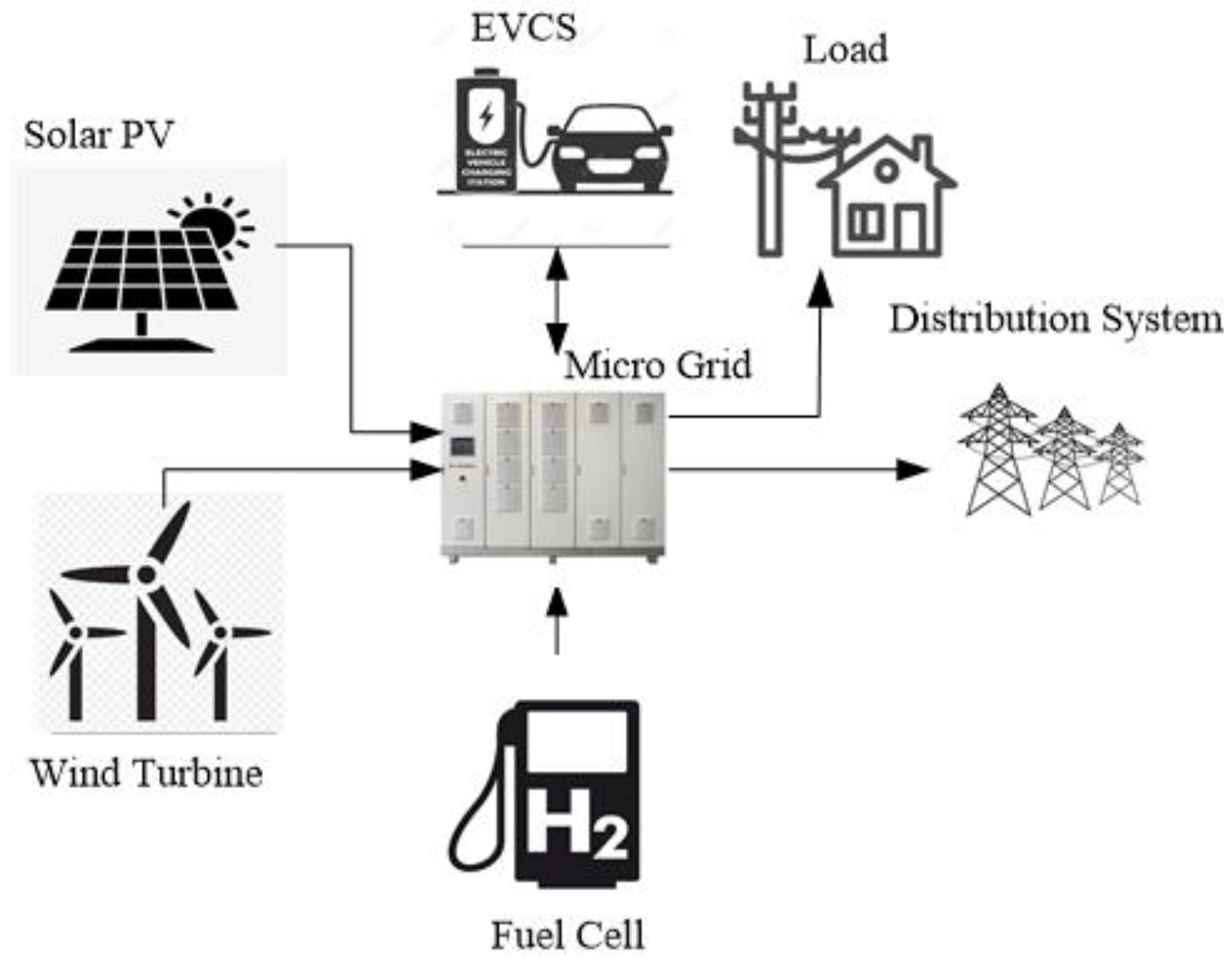
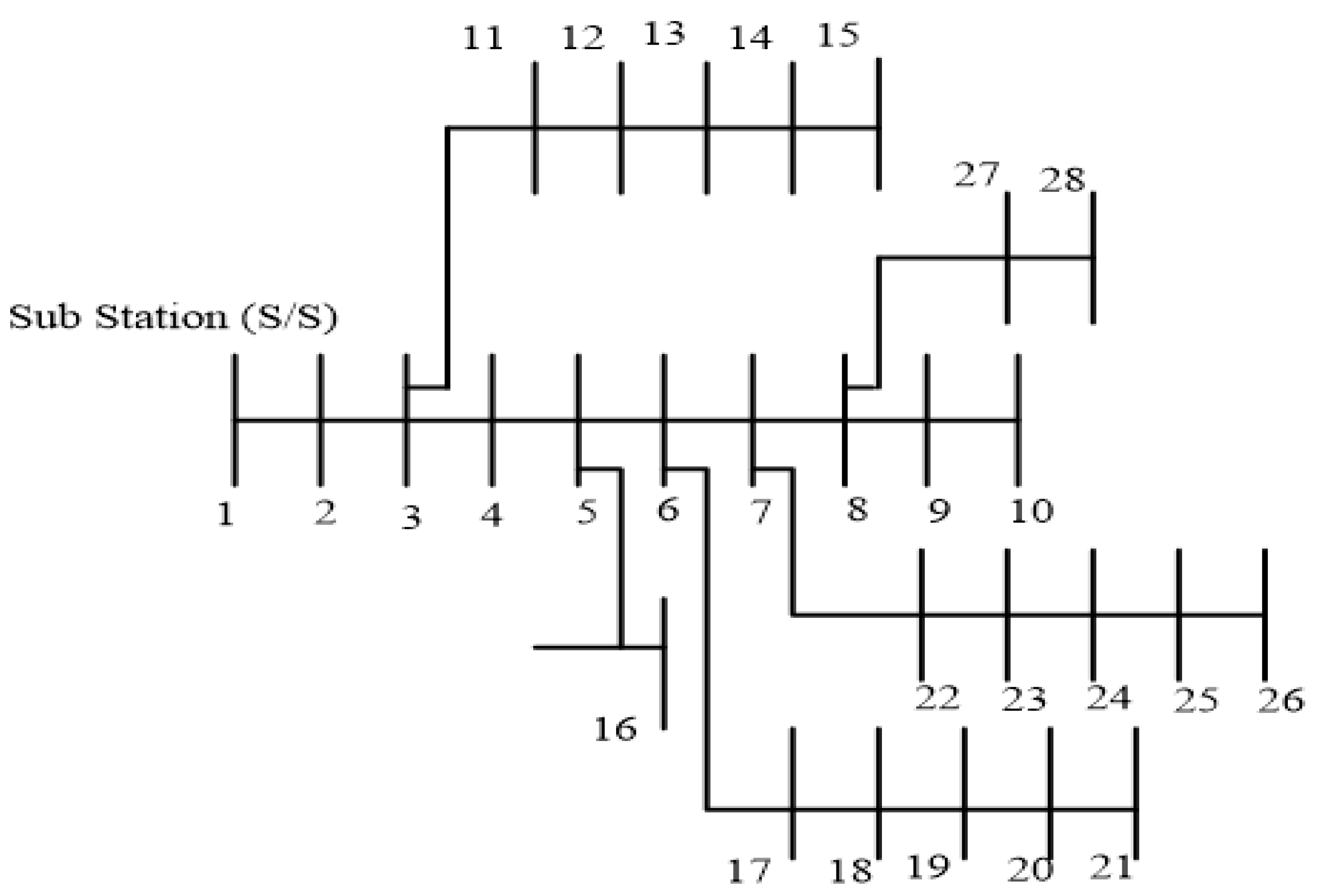
2. System Description
3. Problem Formulation
3.1. Objective Function
3.2. Modelling of Sources
3.2.1. Mathematical Modelling of Fuel Cell
3.2.2. Mathematical Modelling of Solar Irradiance
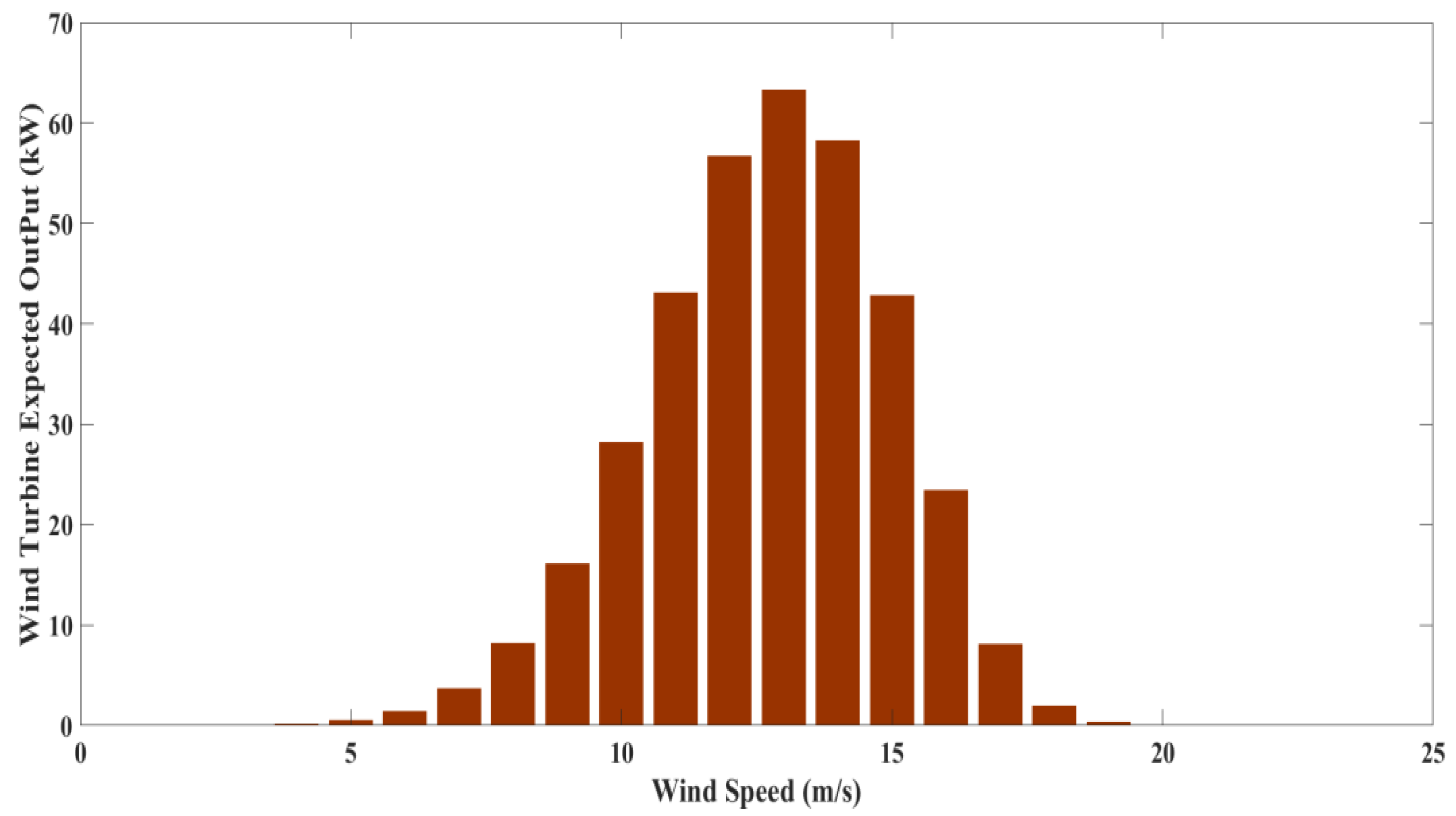
3.2.3. Mathematical Modelling of Wind Speed
3.2.4. Mathematical Modelling of EV Uncertainty
4. Method for Scheduling of RDGs & EVs
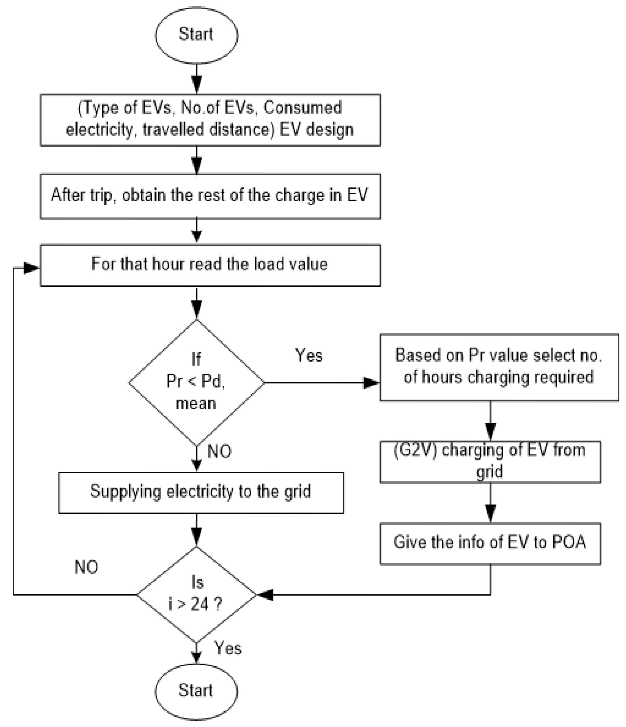
4.1. Conventional and Optimized Charging Methods for EVs
- ○
- The optimized charging method first looks at the type of vehicle, how many vehicles need to be charged, how much each vehicle needs to be charged, and how long the system will run before the next trip.
- ○
- For each hour, the PAR and power ratio is calculated with or without taking EVs into account.
- ○
- (V2G) mode is started if the power ratio is smaller than the average power demand .
- ○
- If the of the specific interval time is larger than the overall power demand , the vehicle can send electricity back to the grid while taking into account the existing SoC.
- ○
- These details will be sent to the POA method every hour to identify the optimal size of renewable DGs.
- ○
- Once the EVs have reached SoC and are available for the next journey, the procedure is completed.
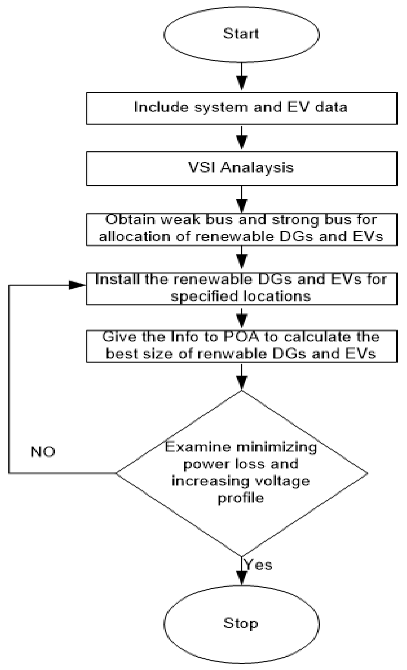
4.2. Best Placement of RDGs and EVCSs Using VSI
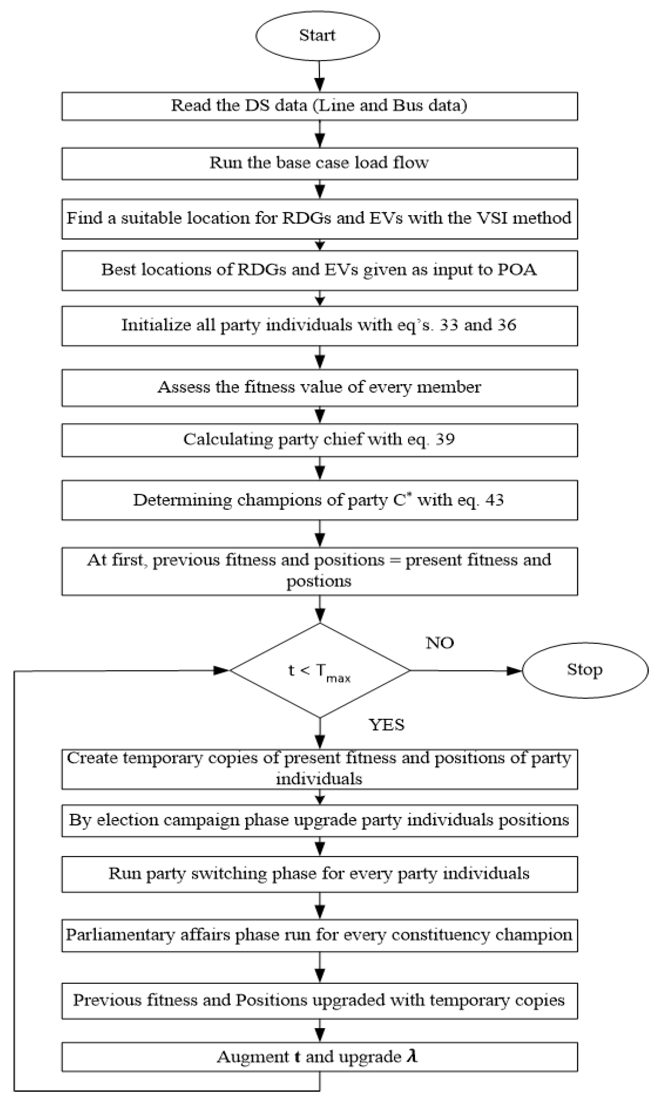
4.3. Renewable DGs and EVs Sizing Finding with Political Optimizer Algorithm (POA)
5. Results and Discussion
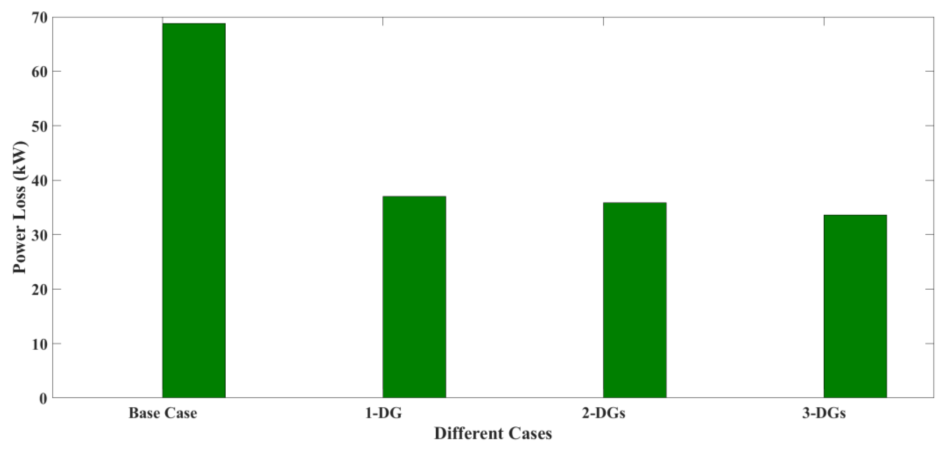
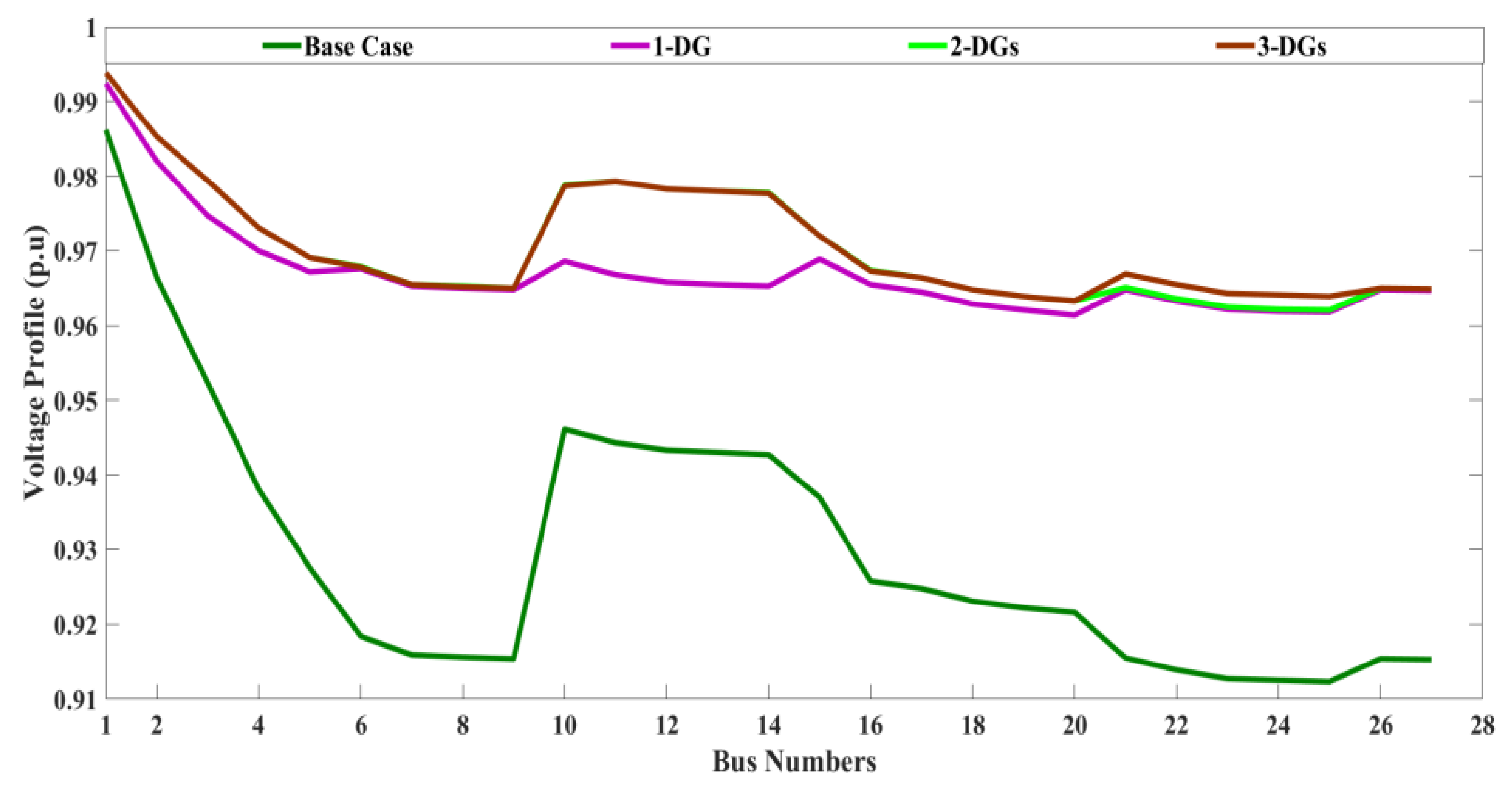
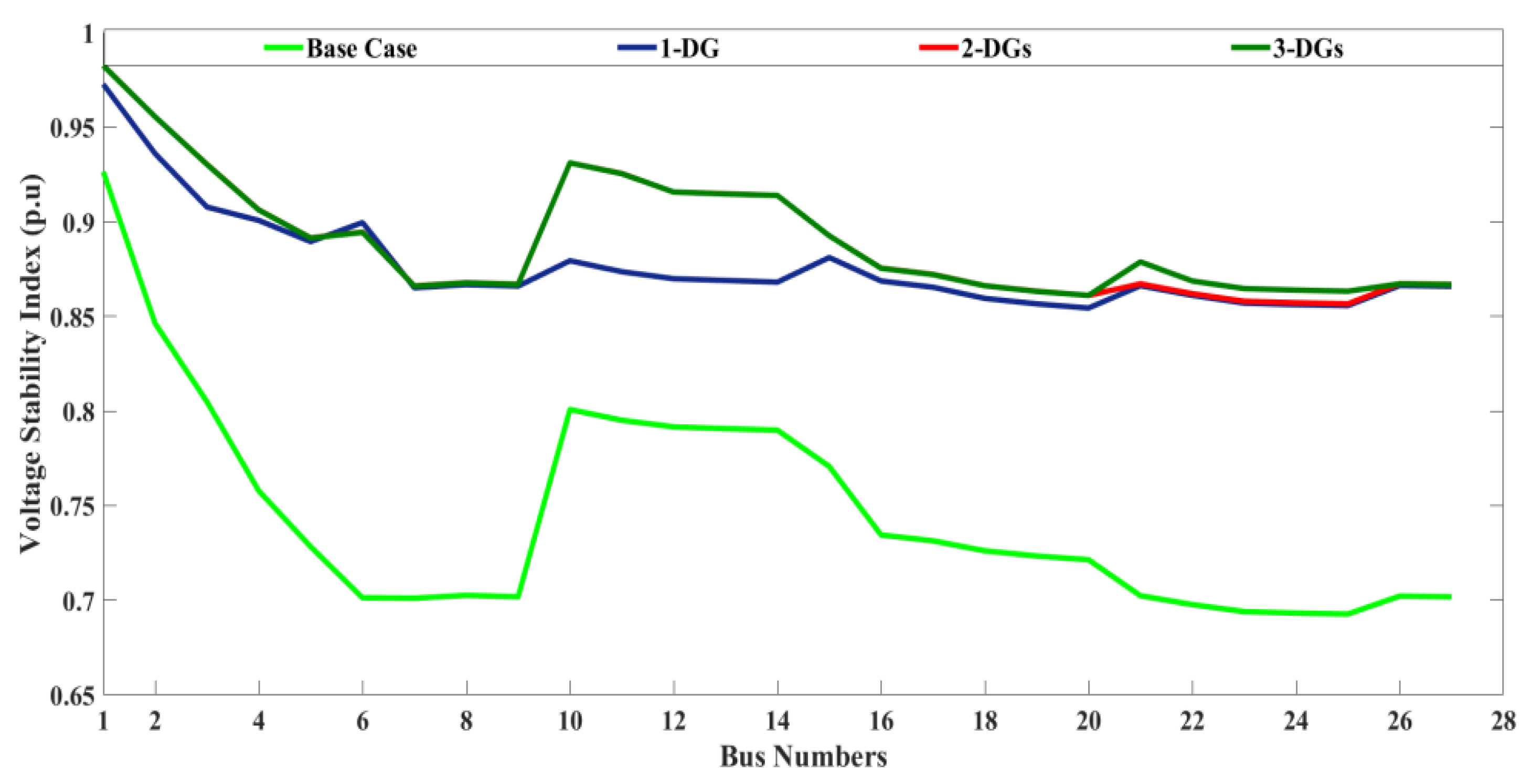
5.1. 28 Indian Real Test System Evaluation without EVs
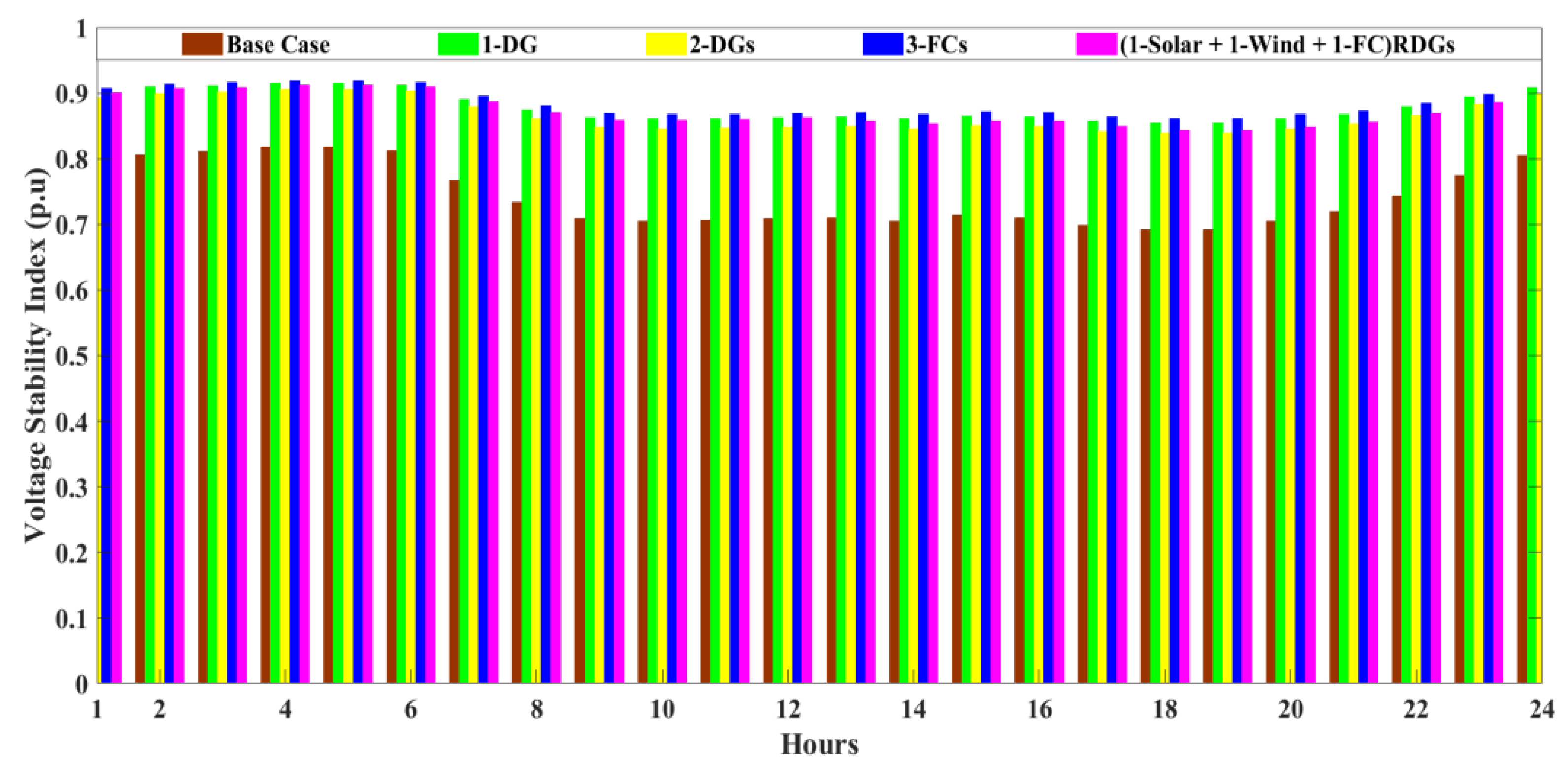
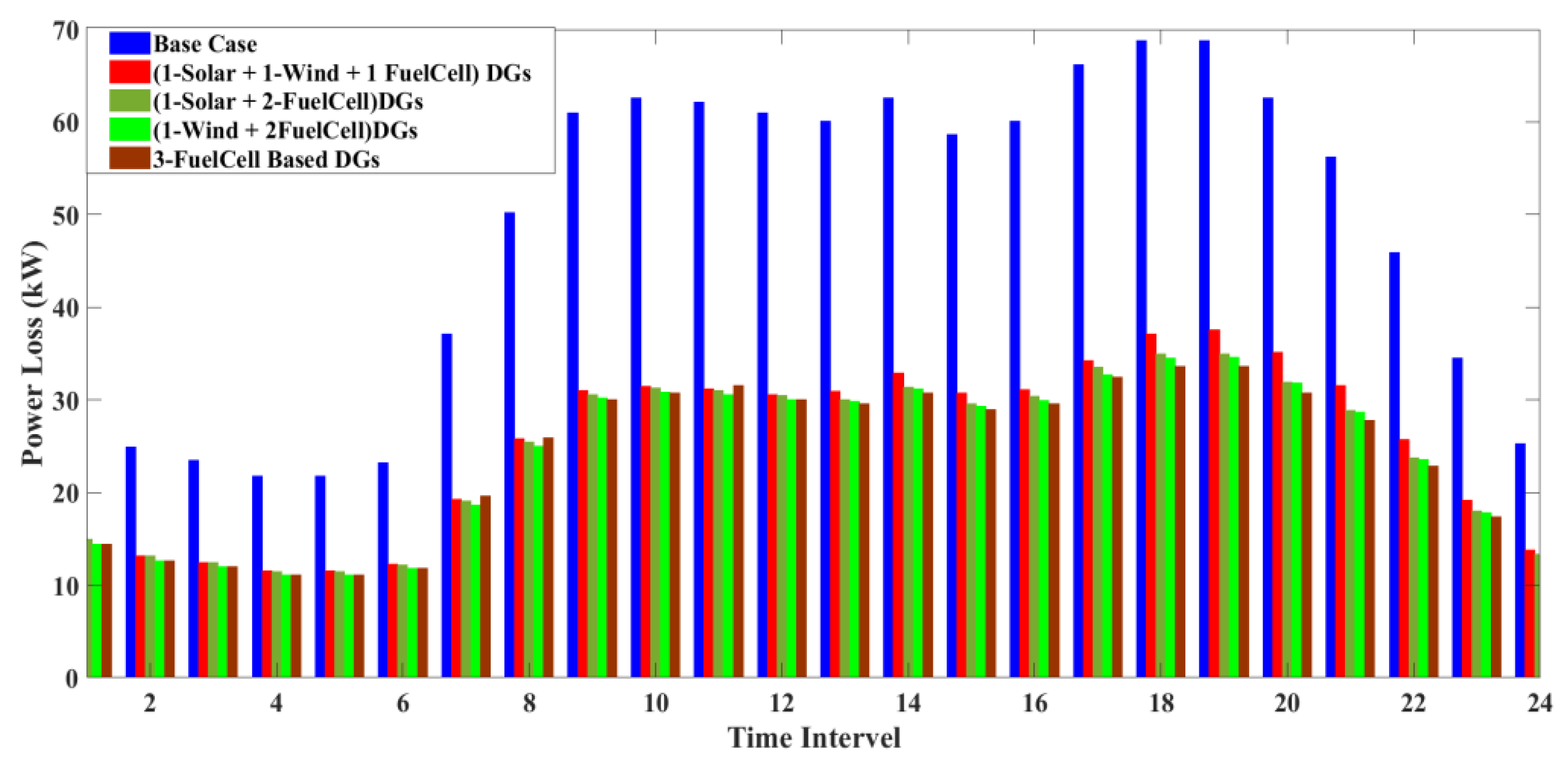
5.2. Optimal Renewable-Based DGs PLoss for a Typical Day without EVs
5.3. 28 Indian Real Test System Evaluation with EVs
- ▪
- There are 60 EVs that ride to work, covering an average daily distance of 30 km, departing at 8:00 a.m. and arriving back at 5:00 p.m.
- ▪
- All EVs must begin their journey with a full charge, and there is no way to recharge between the hours of travel. Furthermore, EVs require significant time to charge their batteries depending on the distance travelled/supplied to the grid.
- ▪
- The technology is also expected to provide a two-way communication system between EVs and the power grid. This channel permits information between them, allowing for combined EV and DG scheduling. As a result, data are transported without delay from one channel to the next.
5.3.1. Conventional Charging Method (CCM)
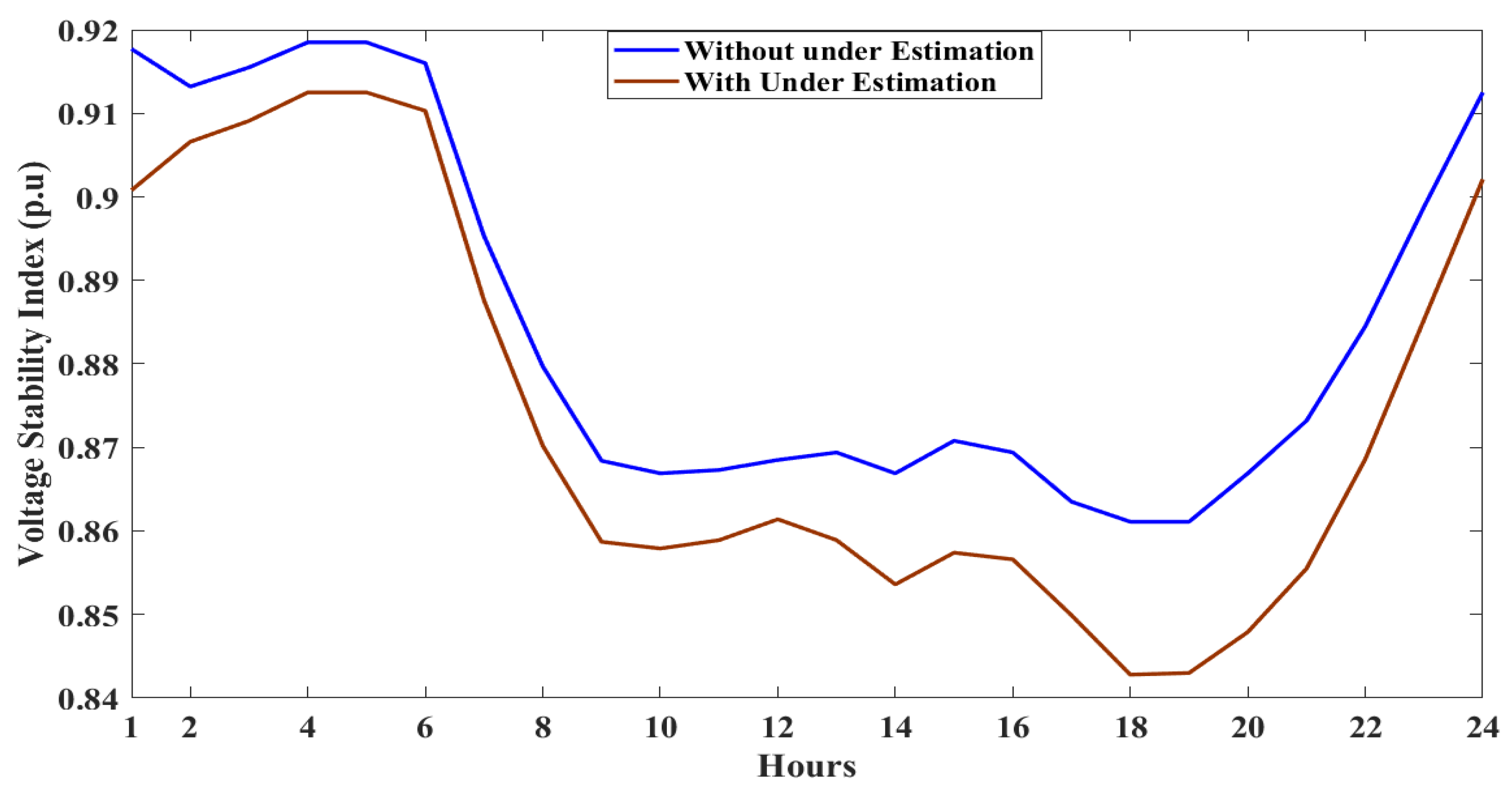
5.3.2. Optimized Charging Method (OCM)
5.3.3. G2V + V2G Method
6. Conclusions
Author Contributions
Funding
Institutional Review Board Statement
Informed Consent Statement
Data Availability Statement
Conflicts of Interest
Nomenclature
| RDGs | Renewable Distributed Generators |
| DS | Distribution System |
| PLoss | Power Loss |
| Probability Distribution Function | |
| VSI | Voltage Stability Index |
| POA | Political Optimizer Algorithm |
| CCM | Conventional Charging Method |
| OCM | Optimized Charging Method |
| DGs | Distributed Generators |
| EVs | Electric Vehicle |
| PEVs | Plug in Electric Vehicles |
| MG | Micro Grids |
| EVCS | Electric Vehicle Charging Station |
| RES | Renewable Energy Resources |
| DERs | Distributed Energy Resources |
| SOFC | Solid Oxide Fuel Cell |
| PEMFC | Proton Exchange Membrane Fuel Cell |
| PV | Photo Voltaic |
| WT | Wind Turbine |
| Probability Distribution Function | |
| FC | Fuel Cell |
| SoC | State of Charge |
| DoC | Decision on Charge |
| PAR | Peak-to0Average Ratio |
| PR | Power Ratio |
| G2V | Grid 2 Vehicle |
| V2G | Vehicle 2 Grid |
| PFC | Fuel Cell output power |
| EFCo | Potential Difference |
| IFC | Current Flow |
| RFC | FC Electrodes have an internal resistance b/w them |
| AFC | FC Electrode Surface Area |
| R, r | Global Gas Constant (J/mol k), internal Resistance (ohm) |
| T | Temperature (kelvin) |
| pH2, pO2, pH2O | Hydrogen, Oxygen and Water (atm) |
| N0, E0 | No.of Cells, Reversible Cell (volts) |
| Beta PDF for Solar Irradiance | |
| αm, βm | Shape Parameters |
| FF | Fill Factor |
| NPVM | Total Number of PV modules |
| Isc | Short Circuit Current |
| Voc | Open Circuit Voltage |
| Tcy | Cell Temperature |
| TA | Ambient Temperature |
| Ki, Kv | Current & Voltage Temperature Coefficients |
| NOT | Nominal Operating Temperature |
| Weibull PDF for Wind Speed | |
| k | Shape Factor |
| c | Scale Factor |
| PWE | Expected Output Power of Wind Turbine |
References
- Shaheen, A.; Elsayed, A.; Ginidi, A.; El-Sehiemy, R.; Elattar, E. Improved Heap-Based Optimizer for DG Allocation in Reconfigured Radial Feeder Distribution Systems. IEEE Syst. J. 2022, 1–10. [Google Scholar] [CrossRef]
- Taha, H.A.; Alham, M.H.; Youssef, H.K.M. Multi-Objective Optimization for Optimal Allocation and Coordination of Wind and Solar DGs, BESSs and Capacitors in Presence of Demand Response. IEEE Access 2022, 10, 16225–16241. [Google Scholar] [CrossRef]
- Suresh, V.; Pachauri, N.; Vigneysh, T. Decentralized control strategy for fuel cell/PV/BESS based microgrid using modified fractional order PI controller. Int. J. Hydrog. Energy 2021, 46, 4417–4436. [Google Scholar] [CrossRef]
- Farrokhabadi, M.; Lagos, D.; Wies, R.W.; Paolone, M.; Liserre, M.; Meegahapola, L. Microgrid Stability Definitions, Analysis, and Examples. IEEE Trans. Power Syst. 2020, 35, 13–29. [Google Scholar] [CrossRef]
- Padhi, P.P.; Nimje, A.A. Distributed Generation: An Overview. Int. Electr. Eng. J. 2012, 3, 607–611. [Google Scholar]
- Rama Prabha, D.; Jayabarathi, T.; Umamageswari, R.; Saranya, S. Optimal location and sizing of distributed generation unit using intelligent water drop algorithm. Sustain. Energy Technol Assess. 2015, 11, 106–113. [Google Scholar] [CrossRef]
- Sanjay, R.; Jayabarathi, T.; Raghunathan, T.; Ramesh, V.; Mithulananthan, N. Optimal allocation of distributed generation using hybrid grey Wolf optimizer. IEEE Access 2017, 5, 14807–14818. [Google Scholar] [CrossRef]
- Uniyal, A.; Sarangi, S. Optimal network reconfiguration and DG allocation using adaptive modified whale optimization algorithm considering probabilistic load flow. Electr. Power Syst. Res. 2021, 192, 106909. [Google Scholar] [CrossRef]
- Huy, T.H.B.; Tran TVan Ngoc Vo, D.; Nguyen, H.T.T. An improved metaheuristic method for simultaneous network reconfiguration and distributed generation allocation. Alexandria Eng. J. 2022, 61, 8069–8088. [Google Scholar] [CrossRef]
- Shaheen, A.; Elsayed, A.; Ginidi, A.; El-Sehiemy, R.; Elattar, E. Reconfiguration of electrical distribution network-based DG and capacitors allocations using artificial ecosystem optimizer: Practical case study. Alexandria Eng. J. 2022, 61, 6105–6118. [Google Scholar] [CrossRef]
- Kayal, P.; Chanda, C.K. Optimal mix of solar and wind distributed generations considering performance improvement of electrical distribution network. Renew Energy 2015, 75, 173–186. [Google Scholar] [CrossRef]
- Home-Ortiz, J.M.; Pourakbari-Kasmaei, M.; Lehtonen, M.; Sanches Mantovani, J.R. Optimal location-allocation of storage devices and renewable-based DG in distribution systems. Electr. Power Syst. Res. 2019, 172, 11–21. [Google Scholar] [CrossRef]
- Jafar-Nowdeh, A.; Babanezhad, M.; Arabi-Nowdeh, S.; Naderipour, A.; Kamyab, H.; Abdul-Malek, Z.; Ramachandaramurthy, V.K. Meta-heuristic matrix moth–flame algorithm for optimal reconfiguration of distribution networks and placement of solar and wind renewable sources considering reliability. Environ. Technol. Innov. 2020, 20, 101118. [Google Scholar] [CrossRef]
- Rathore, A.; Patidar, N.P. Optimal sizing and allocation of renewable based distribution generation with gravity energy storage considering stochastic nature using particle swarm optimization in radial distribution network. J. Energy Storage 2021, 35, 102282. [Google Scholar] [CrossRef]
- Hassan, A.S.; Sun, Y.; Wang, Z. Water, Energy and Food Algorithm with Optimal Allocation and Sizing of Renewable Distributed Generation for Power Loss Minimization in Distribution Systems (WEF). Energies 2022, 15, 2242. [Google Scholar] [CrossRef]
- Liu, J.P.; Zhang, T.X.; Zhu, J.; Ma, T.N. Allocation optimization of electric vehicle charging station (EVCS) considering with charging satisfaction and distributed renewables integration. Energy 2018, 164, 560–574. [Google Scholar] [CrossRef]
- Hariri, A.M.; Hejazi, M.A.; Hashemi-Dezaki, H. Reliability optimization of smart grid based on optimal allocation of protective devices, distributed energy resources, and electric vehicle/plug-in hybrid electric vehicle charging stations. J. Power Sour. 2019, 436, 226824. [Google Scholar] [CrossRef]
- Gupta, K.; Achathuparambil Narayanankutty, R.; Sundaramoorthy, K.; Sankar, A. Optimal location identification for aggregated charging of electric vehicles in solar photovoltaic powered microgrids with reduced distribution losses. In Energy Sources, Part A: Recovery, Utilization and Environmental Effects; Taylor & Francis: Oxfordshire, UK, 2020; pp. 1–16. [Google Scholar]
- Pal, A.; Bhattacharya, A.; Chakraborty, A.K. Allocation of electric vehicle charging station considering uncertainties. Sustain. Energy Grids Netw. 2021, 25, 100422. [Google Scholar] [CrossRef]
- Li, C.; Zhang, L.; Ou, Z.; Wang, Q.; Zhou, D.; Ma, J. Robust model of electric vehicle charging station location considering renewable energy and storage equipment. Energy 2022, 238, 121713. [Google Scholar] [CrossRef]
- Padullés, J.; Ault, G.W.; McDonald, J.R. Integrated SOFC plant dynamic model for power systems simulation. J. Power Sources 2000, 86, 495–500. [Google Scholar] [CrossRef]
- Lavorante, M.J.; Sanguinetti, A.R.; Fasoli, H.J.; Aiello, R.M. Equation for General Description of Power Behaviour in Fuel Cells. J. Renew Energy 2018, 2018, 2678050. [Google Scholar] [CrossRef] [Green Version]
- Ranjan, R.; Venkatesh, B.; Das, D. Voltage stability analysis of radial distribution networks. Electr. Power Compon. Syst. 2003, 31, 501–511. [Google Scholar] [CrossRef]
- Borji, A. A new global optimization algorithm inspired by parliamentary political competitions. In Lecture Notes in Computer Science; including Subser Lecture Notes Artificial Intelligence Lecture Notes Bioinformatics; Springer: Berlin, Germany, 2007; pp. 61–71. [Google Scholar]
- Askari, Q.; Younas, I.; Saeed, M. Political Optimizer: A novel socio-inspired meta-heuristic for global optimization. Knowl. Based Syst. 2020, 195, 105709. [Google Scholar] [CrossRef]
- Zhu, A.; Gu, Z.; Hu, C.; Niu, J.; Xu, C.; Li, Z. Political optimizer with interpolation strategy for global optimization. PLoS ONE 2021, 16, e0251204. [Google Scholar]


| Description | Specifications | Ratings |
|---|---|---|
| Solar PV | Solar panel | 220 W |
| Ambient Temperature (Ta) | 30.76 °C | |
| Nominal cell operating temperature (Not) | 43 °C | |
| Open Circuit Voltage | 36.96 V | |
| Short Circuit Current | 8.38 A | |
| Wind Turbine | Wind Turbine | 3000 kW |
| Cut-in Speed | 3.5 m/s | |
| Cut-out Speed | 25 m/s | |
| Hub height | 66 m | |
| Rated Speed | 15 m/s | |
| EVs | E.V Capacity or Battery | 16 kWh |
| No. of EVs | 60 | |
| SoCmin | 0.2 | |
| SoCmax | 0.9 | |
| Avg. power consumption per km | 0.175 kWh/km | |
| Avg. distance travelled by each EV | 30 km |
| Different Cases | Bus. No | DG Size (kW) | PLoss (kW) | Vmin (p.u) | VSImin (p.u) | % Red of Ploss |
|---|---|---|---|---|---|---|
| Base Case | NA | NA | 68.8189 | 0.9123 | 0.6927 | NA |
| 1-DG | 7 | 583.0954 | 37.0066 | 0.9615 | 0.8545 | 46.22 |
| 2-DGs | 9 12 | 403.2352 272.0916 | 35.8397 | 0.9572 | 0.8395 | 47.92 |
| 3-DGs | 7 12 22 | 334.2644 230.5484 145.6193 | 33.6501 | 0.9633 | 0.8611 | 51.10 |
| Different Loads | Without DG PLoss (kW) | With DG PLoss (kW) | DG Size in kW | Vmin (p.u) | VSImin (p.u) | % Red of PLoss |
|---|---|---|---|---|---|---|
| Half Load (0.5) | 15.8508 | 8.132 | 162.8245 111.5187 72.5212 | 0.982 | 0.9299 | 48.6965 |
| Full Load (1.0) | 68.8189 | 33.6501 | 334.2578 230.5428 145.6313 | 0.9633 | 0.8611 | 51.1086 |
| Heavy Load (1.1) | 84.7675 | 41.0029 | 369.6675 255.3580 160.3221 | 0.9595 | 0.8475 | 51.6289 |
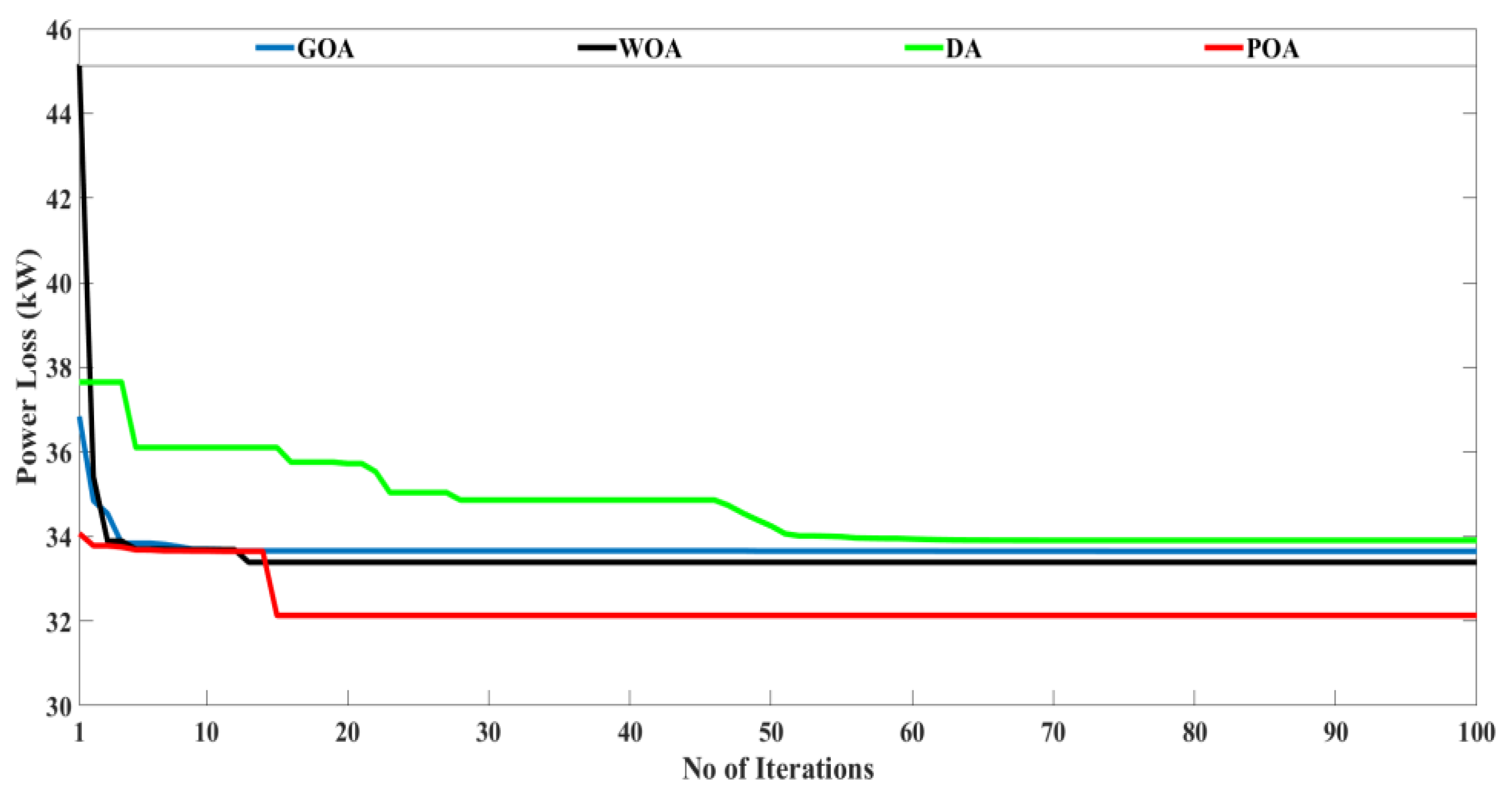
| Different Methods | DG Size (kW) | PLoss (kW) | Vmin (p.u) | VSImin (p.u) | Time (s) |
|---|---|---|---|---|---|
| GOA | 334.5567 230.4150 145.4057 | 33.6501 | 0.9639 | 0.8615 | 13.7916 |
| WOA | 182.5131 262.1375 265.0773 | 33.9388 | 0.9614 | 0.8542 | 13.6241 |
| DA | 332.81 235.1821 145.1592 | 33.6513 | 0.9634 | 0.8612 | 13.7491 |
| POA | 222.0523 220.5258 256.781 | 32.1337 | 0.9633 | 0.8611 | 13.5817 |
| Hours | DG1 (kW) | DG2 (kW) | DG3 (kW) |
|---|---|---|---|
| 1 | 217.0467 | 148.979 | 95.977 |
| 2 | 203.4865 | 139.5917 | 90.1536 |
| 3 | 197.7144 | 135.6158 | 87.6951 |
| 4 | 190.3307 | 130.4985 | 84.4631 |
| 5 | 190.3452 | 130.4988 | 84.455 |
| 6 | 196.3892 | 134.681 | 87.1098 |
| 7 | 247.3955 | 170.0333 | 108.9991 |
| 8 | 286.7203 | 197.383 | 125.6688 |
| 9 | 315.2901 | 217.3105 | 137.6994 |
| 10 | 319.1438 | 219.9935 | 139.3215 |
| 11 | 318.0901 | 219.2612 | 138.8779 |
| 12 | 315.3042 | 217.3044 | 137.6907 |
| 13 | 312.8509 | 215.5912 | 136.6694 |
| 14 | 319.1481 | 219.987 | 139.3158 |
| 15 | 309.3421 | 213.1604 | 135.2089 |
| 16 | 312.8398 | 215.5972 | 136.6844 |
| 17 | 327.9367 | 226.1077 | 142.9729 |
| 18 | 334.2414 | 230.5464 | 145.6437 |
| 19 | 334.2334 | 230.5656 | 145.6326 |
| 20 | 319.1343 | 219.9909 | 139.3344 |
| 21 | 303.0699 | 208.7601 | 132.5754 |
| 22 | 274.6099 | 188.9348 | 120.549 |
| 23 | 238.8566 | 164.0718 | 105.333 |
| 24 | 204.8351 | 140.523 | 90.7436 |
| Hour | RDG1 (kW) | RDG2 (kW) | RDG3 (kW) | CCM EVs Size (kW) | OCM EVs Size (kW) |
|---|---|---|---|---|---|
| 1 | 0 | 168.6979 | 275.711 | 0 | 0 |
| 2 | 0 | 158.0734 | 258.6207 | 0 | 0 |
| 3 | 0 | 137.9663 | 257.2959 | 0 | 0 |
| 4 | 0 | 132.3059 | 247.9305 | 0 | 164.9124 93.6902 84.4630 |
| 5 | 0 | 122.8699 | 251.5886 | 0 | 164.8767 93.6953 84.5098 |
| 6 | 23.0397 | 111.9504 | 244.8535 | 0 | 171.0092 97.8715 87.0779 |
| 7 | 36.7313 | 142.016 | 301.0115 | 0 | 0 |
| 8 | 58.2045 | 141.6904 | 344.1369 | 0 | 0 |
| 9 | 75.3447 | 159.4687 | 366.7543 | 0 | 0 |
| 10 | 90.6312 | 194.2686 | 345.965 | 0 | 0 |
| 11 | 89.5447 | 216.6312 | 337.0031 | 0 | 0 |
| 12 | 94.1047 | 232.4594 | 322.7771 | 0 | 0 |
| 13 | 47.0657 | 143.4683 | 393.0898 | 0 | 0 |
| 14 | 45.1035 | 95.7511 | 423.6257 | 0 | 0 |
| 15 | 46.5414 | 105.5039 | 401.988 | 0 | 0 |
| 16 | 38.4655 | 136.6521 | 403.009 | 0 | 0 |
| 17 | 20.2208 | 142.6663 | 439.822 | 0 | 0 |
| 18 | 0 | 69.5131 | 495.9151 | 309.0081 193.6312 145.6272 | 0 |
| 19 | 0 | 53.5084 | 502.79 | 308.9711 193.6310 145.6605 | 0 |
| 20 | 0 | 16.3767 | 493.297 | 293.8829 183.0712 139.3334 | 0 |
| 21 | 0 | 23.4579 | 465.6374 | 0 | 0 |
| 22 | 0 | 29.9008 | 418.8243 | 0 | 0 |
| 23 | 0 | 42.4956 | 357.8433 | 0 | 0 |
| 24 | 0 | 64.0545 | 296.7647 | 0 | 0 |
| Hours | Base Case PLoss (kW) | (1-Solar + 1-Wind + 1-FC) DG PLoss (KW) | (1-Solar + 2- FC) DGs PLoss (kW) | (1-Wind + 2-FC) DGs PLoss (kW) | 3-FC Based DGs PLoss (kW) |
|---|---|---|---|---|---|
| 1 | 28.4096 | 14.8999 | 14.8999 | 14.3656 | 14.3654 |
| 2 | 24.9163 | 13.1132 | 13.1132 | 12.6471 | 12.6454 |
| 3 | 23.5076 | 12.4037 | 12.3899 | 11.9522 | 11.949 |
| 4 | 21.751 | 11.4991 | 11.4855 | 11.082 | 11.0781 |
| 5 | 21.751 | 11.5209 | 11.4855 | 11.0936 | 11.0781 |
| 6 | 23.1827 | 12.21 | 12.1192 | 11.8086 | 11.7881 |
| 7 | 37.1053 | 19.2422 | 19.057 | 18.6662 | 19.6057 |
| 8 | 50.1845 | 25.8305 | 25.4155 | 25.0255 | 25.8845 |
| 9 | 61.0107 | 31.0461 | 30.5826 | 30.1852 | 30.0013 |
| 10 | 62.5568 | 31.4642 | 31.2581 | 30.8709 | 30.7265 |
| 11 | 62.1329 | 31.1711 | 31.0124 | 30.6008 | 31.5278 |
| 12 | 61.0107 | 30.5748 | 30.4865 | 30.0558 | 30.0013 |
| 13 | 60.0386 | 30.9146 | 30.0495 | 29.8682 | 29.5446 |
| 14 | 62.5568 | 32.9205 | 31.3512 | 31.1937 | 30.7265 |
| 15 | 58.6655 | 30.7236 | 29.5805 | 29.3434 | 28.8987 |
| 16 | 60.0386 | 31.0588 | 30.3959 | 29.9069 | 29.5446 |
| 17 | 66.1549 | 34.2544 | 33.5202 | 32.6922 | 32.409 |
| 18 | 68.8189 | 37.1484 | 34.9673 | 34.4751 | 33.6501 |
| 19 | 68.8189 | 37.5329 | 34.9673 | 34.553 | 33.6501 |
| 20 | 62.5568 | 35.148 | 31.9214 | 31.8015 | 30.7265 |
| 21 | 56.2403 | 31.5144 | 28.8271 | 28.6619 | 27.7552 |
| 22 | 45.9301 | 25.717 | 23.7262 | 23.5273 | 22.8544 |
| 23 | 34.5317 | 19.2026 | 18.0085 | 17.7884 | 17.3566 |
| 24 | 25.2543 | 13.8061 | 13.2865 | 13.0294 | 12.8123 |
| Total PLoss | 1147.1245 | 604.917 | 583.9069 | 575.1945 | 570.5798 |
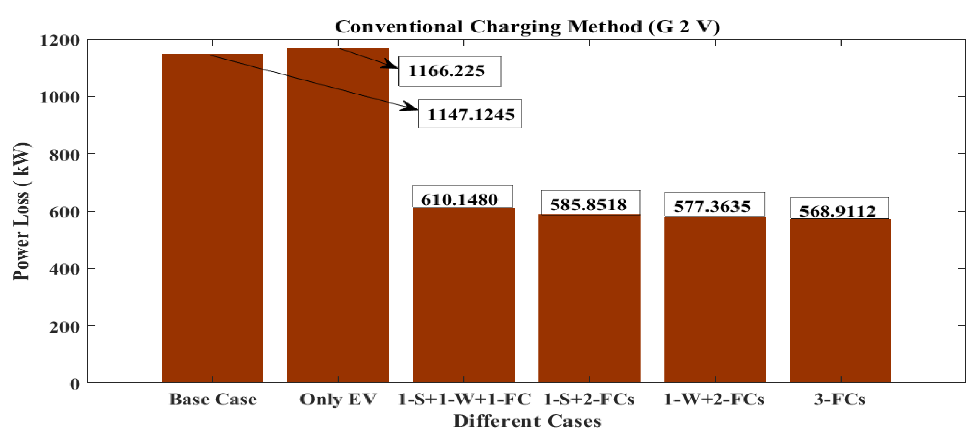
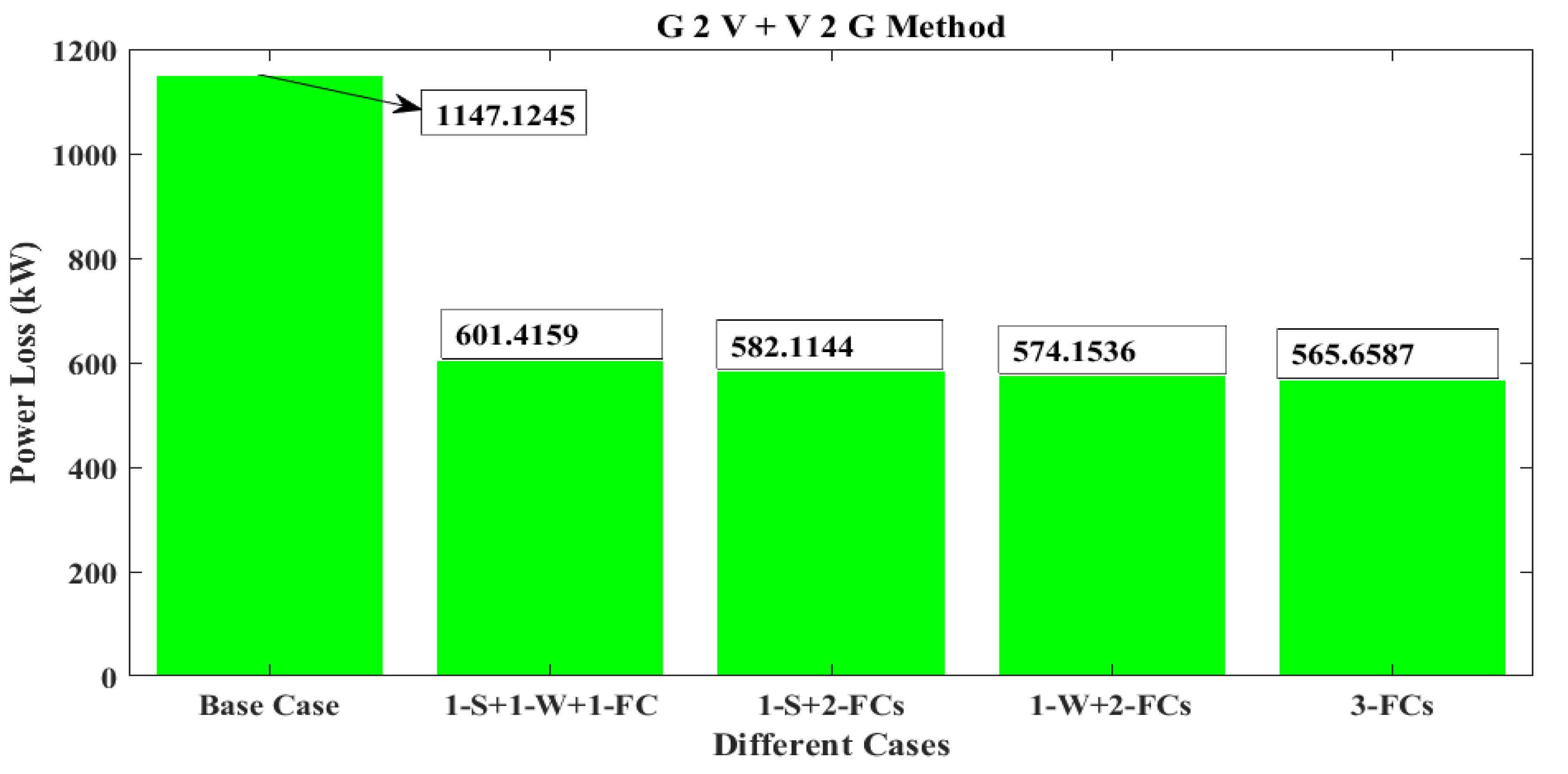
| Different Cases | Total PLoss in (kW) | |
|---|---|---|
| Base Case | 1147.1245 | |
| Conventional EV Charging Method (G2V) | Only EVs | 1166.225 |
| (1-S + 1-W+ 1-FC) DGs with EVs (G to V) | 610.1480 | |
| (1-S + 2-FC) DGs with EVs (G to V) | 585.8518 | |
| (1-W + 2-FC) DGs with EVs (G to V) | 577.3635 | |
| 3-FC Based DGs with EVs (G to V) | 568.9112 | |
| Optimised EV Charging Method (G2V) | Only EVs | 1157.8053 |
| (1-S + 1-W+ 1-FC) DGs with EVs (G to V) | 606.3257 | |
| (1-S + 2-FC) DG with EVs (G to V) | 584.6451 | |
| (1-W + 2-FC) DG with EVs (G to V) | 576.3496 | |
| 3-FC Based DGs with EVs (G to V) | 567.9729 | |
| (1-S + 1-W + 1-FC) DG EV Charging Method (G2V + V2G) | 601.4159 | |
| (1-S + 2-FC) DG EV Charging Method (G to V + V to G) | 582.1144 | |
| (1-W + 2-FC) DG EV Charging Method (G to V + V to G) | 574.1536 | |
| (3-FC) DGs EV Charging Method (G to V + V to G) | 565.6587 | |
Publisher’s Note: MDPI stays neutral with regard to jurisdictional claims in published maps and institutional affiliations. |
© 2022 by the authors. Licensee MDPI, Basel, Switzerland. This article is an open access article distributed under the terms and conditions of the Creative Commons Attribution (CC BY) license (https://creativecommons.org/licenses/by/4.0/).
Share and Cite
Dharavat, N.; Sudabattula, S.K.; Velamuri, S.; Mishra, S.; Sharma, N.K.; Bajaj, M.; Elgamli, E.; Shouran, M.; Kamel, S. Optimal Allocation of Renewable Distributed Generators and Electric Vehicles in a Distribution System Using the Political Optimization Algorithm. Energies 2022, 15, 6698. https://doi.org/10.3390/en15186698
Dharavat N, Sudabattula SK, Velamuri S, Mishra S, Sharma NK, Bajaj M, Elgamli E, Shouran M, Kamel S. Optimal Allocation of Renewable Distributed Generators and Electric Vehicles in a Distribution System Using the Political Optimization Algorithm. Energies. 2022; 15(18):6698. https://doi.org/10.3390/en15186698
Chicago/Turabian StyleDharavat, Nagaraju, Suresh Kumar Sudabattula, Suresh Velamuri, Sachin Mishra, Naveen Kumar Sharma, Mohit Bajaj, Elmazeg Elgamli, Mokhtar Shouran, and Salah Kamel. 2022. "Optimal Allocation of Renewable Distributed Generators and Electric Vehicles in a Distribution System Using the Political Optimization Algorithm" Energies 15, no. 18: 6698. https://doi.org/10.3390/en15186698
APA StyleDharavat, N., Sudabattula, S. K., Velamuri, S., Mishra, S., Sharma, N. K., Bajaj, M., Elgamli, E., Shouran, M., & Kamel, S. (2022). Optimal Allocation of Renewable Distributed Generators and Electric Vehicles in a Distribution System Using the Political Optimization Algorithm. Energies, 15(18), 6698. https://doi.org/10.3390/en15186698