
Optimal Sizing and Location of Photovoltaic Generation and Energy Storage Systems in an Unbalanced Distribution System

 ,
,  and
and
Abstract
:1. Introduction
2. Problem Formulation
2.1. Objective Function
| : | the objective function for the evaluation of the issue of sizing and locating. | |
| : | the function of system loss, including lines and transformers loss. | |
| : | the summation function of the system voltage unbalance rate. | |
| : | the summation function of the system voltage variation rate. | |
| : | the installation cost of the PVGS. | |
| : | the installation cost of the BESS. | |
| : | the three-phase voltage unbalance rate on bus b at hour t. | |
| : | the three-phase voltage variation rate on bus b at hour t. | |
| : | the weighting parameter of the line power loss, (NT$/kW). | |
| : | the weighting parameter of the transformer power loss, (NT$/kW). | |
| : | the penalty parameter of the voltage unbalance rate at hour t (NT$). VUR_lim is the limitation of the voltage unbalance ratio on each load bus. | |
| : | the penalty parameter of the voltage variation rate on bus b at hour t (NT$). d = | |
| e | : | the unit price of PVGS installation in NT$/kW. |
| f | : | the unit price of BESS installation in NT$/kWh. |
| : | the total system line loss at hour t (kW). | |
| : | the total system transformer loss at hour t (kW). | |
| : | the PVGS capacity on the chosen bus n; it must be an integer in multiple numbers of 50 kW. | |
| : | the BESS capacity on the chosen bus m; it must be an integer in multiple numbers of 50 kW. | |
| NS | : | the set of the chosen feed-in bus number of the PVGS. |
| NST | : | the set of the chosen feed-in bus number of the BESS. |
| NB | : | the maximum system bus number. |
2.2. Constraints
- (1)
- Equality constraints:
- (2)
- Inequality constraints:
3. Solution Algorithm—RGA-ASCM
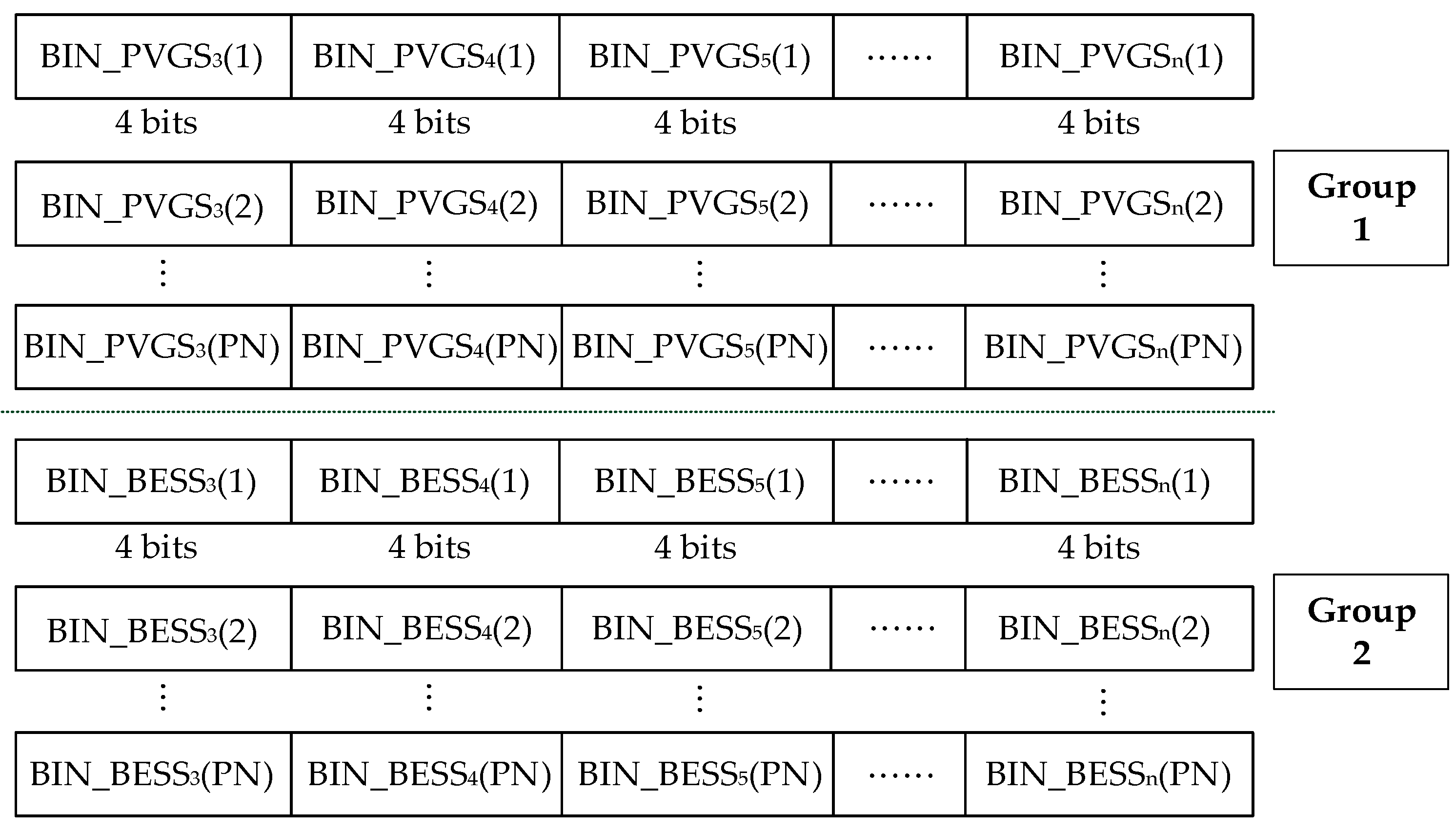
3.1. Encoding of Genes and Chromosomes
3.2. Fitness Function Evaluation
3.3. Production of the Offspring
- SCM Scheme [12]
- 2.
- ICM scheme
- (1)
- Select two parents randomly to produce offspring according to the following:
- (a)
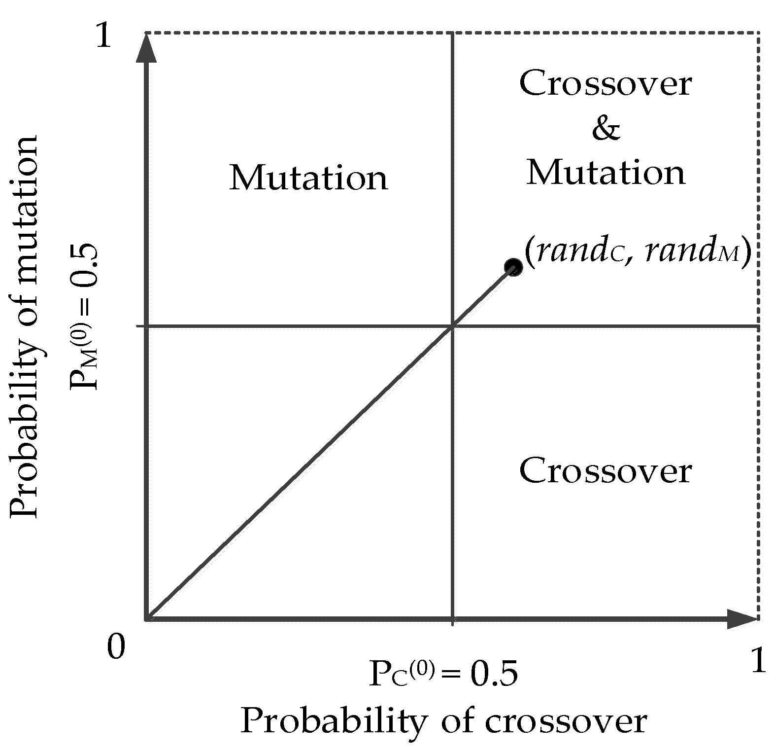
- If randC < PC(g) and randM < PM(g), without executing the crossover and mutation processes;
- (b)
- If randC ≥ PC(g) and randM < PM(g), only the crossover process is executed;
- (c)
- If randC < PC(g) and randM ≥ PM(g), only the mutation process is executed;
- (d)
- If randC ≥ PC(g) and randM ≥ PM(g), with the crossover and mutation process executed sequentially.
| randC | : | the uniform random number in (0,1) for crossover. |
| randM | : | the uniform random number in (0,1) for mutation. |
| g | : | the current generation numbers. |
| PC(g) | : | the control parameter crossover process with initial value PC(0) = 0.5 and 0 ≤ PC ≤ 1. |
| PM(g) | : | the control parameter mutation process with initial value PM(0) = 0.5 and 0 ≤ PM ≤ 1. |
- (2)
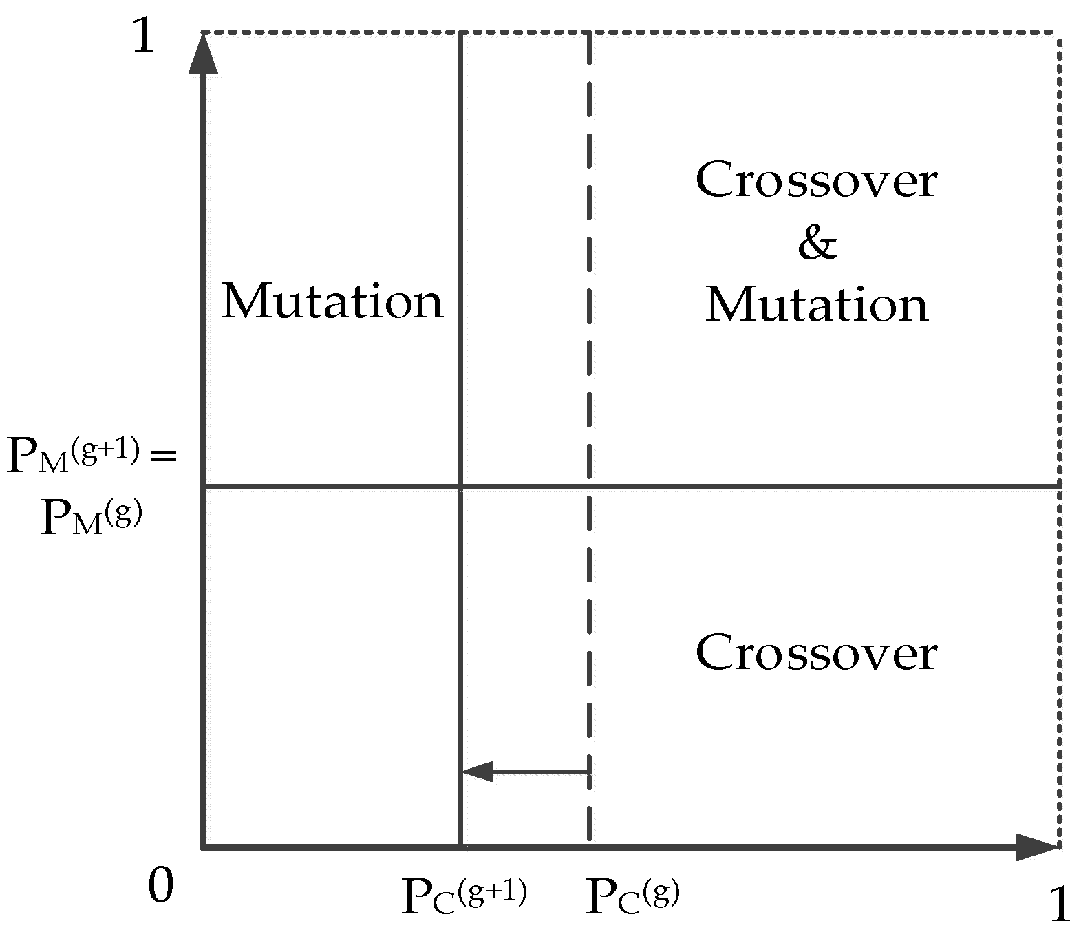
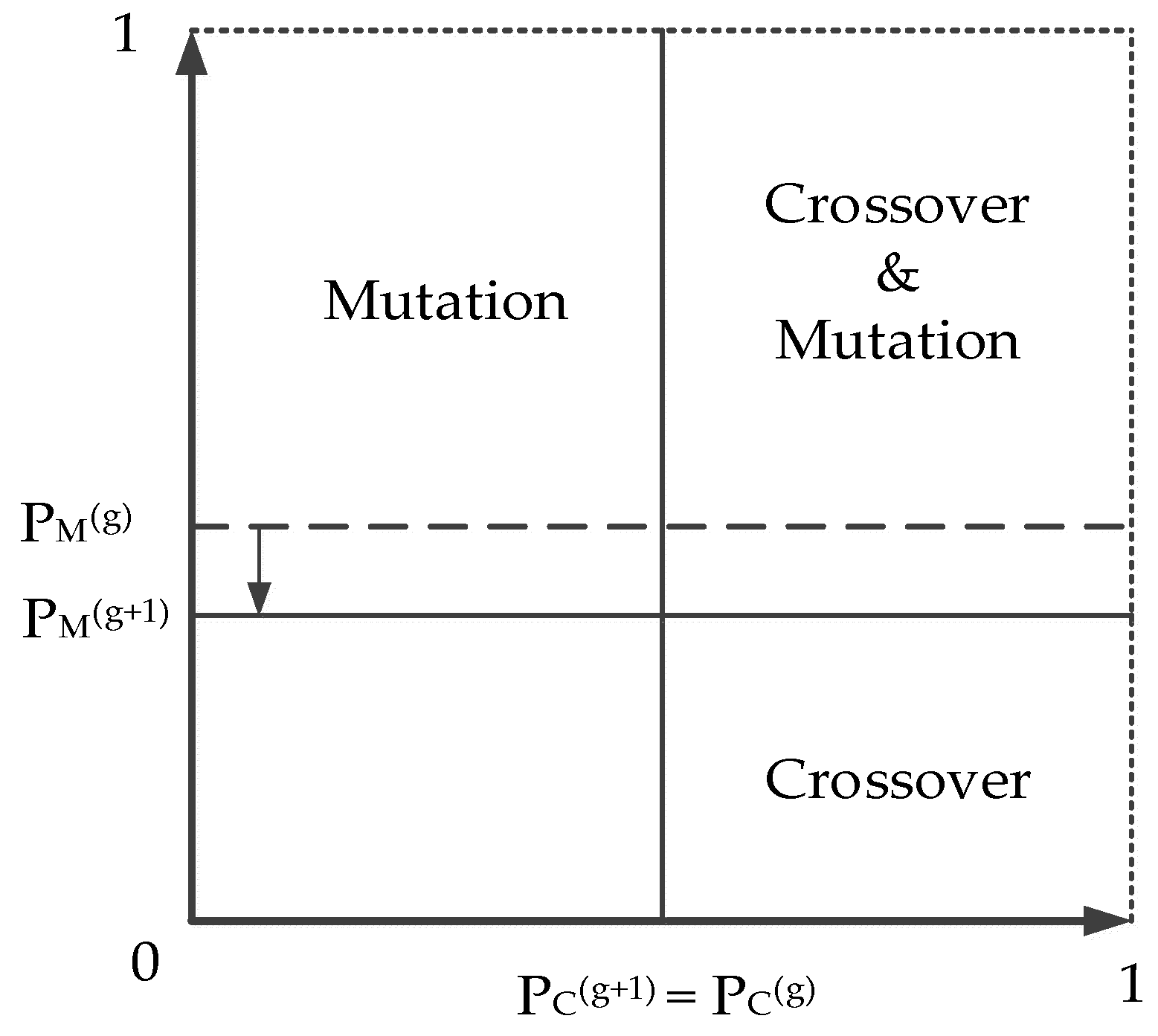
- A competition mechanism is implemented in the searching process according to the fitness score. For instance, if the best current solution comes from both the crossover and mutation processes, there is more likelihood for this procedure to generate better offspring for the next population. The area of the crossover and mutation procedure must be increased by reducing PC(g) and PM(g) to expand the probability, as shown in Figure 3.
- (3)
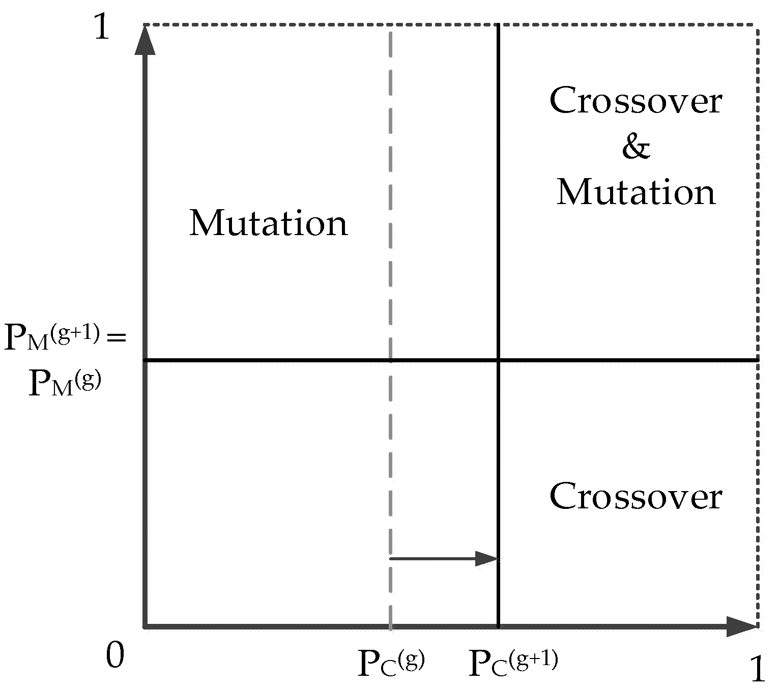
- If the best fitness of generation g-1 is greater than that of generation g (i.e., comes from only the crossover procedure), the control parameter will decrease by using Equation (15). Conversely, if comes from the crossover, the control parameters will increase by employing Equation (17). In this situation, the control parameter PM is fixed. The probability variation of the crossover is illustrated in Figure 5 and Figure 6.
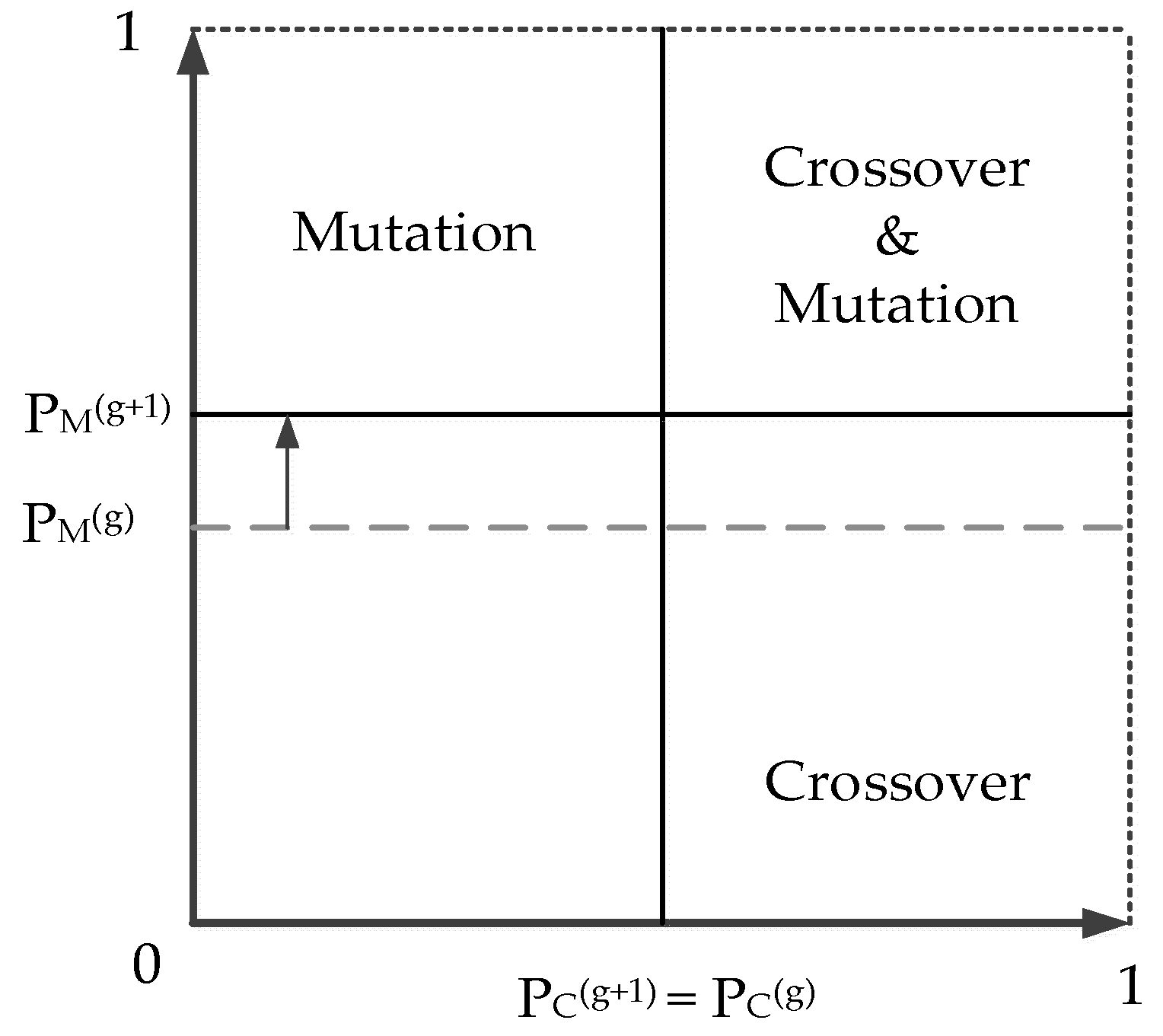
- (4)
- If the best fitness of generation g-1 is greater than that of generation g (i.e., comes only from the mutation procedure), the control parameter will decrease by employing Equation (16). Conversely, if , the control parameters will increase by employing Equation (18). In this situation, the control parameter PC is fixed. The probability variation is illustrated in Figure 7 and Figure 8.
3.4. Tabu List
- The solutions just visited, except for the best solution in the current generation;
- Any local optima ever visited;
- The chromosomes violate the constraints;
- The solution space cannot accord with the bargain condition.
3.5. Elitism Selection
3.6. Stopping Rule
- Step 1. Data Collection.
- Step 2. Randomly generate the multiple integer numbers of the PVGS and BESS capacity;
- Step 3. Coding—decimal to four-bit binary digits;
- Step 4. ICM process;
- Step 5. Decoding—four-bit binary digits to decimal;
- Step 6. Check if the chromosomes are in the Tabu list;
- Yes: Go to Step 4; No: Go to Step 7;
- Step 7. Elite selection;
- Step 8. Did the convergence occur? Or is the maximum generation number reached?
- Yes: Go to Step 9; No: Go to Step 4;
- Step 9. List the optimal planning combinations;
- Step 10. End.
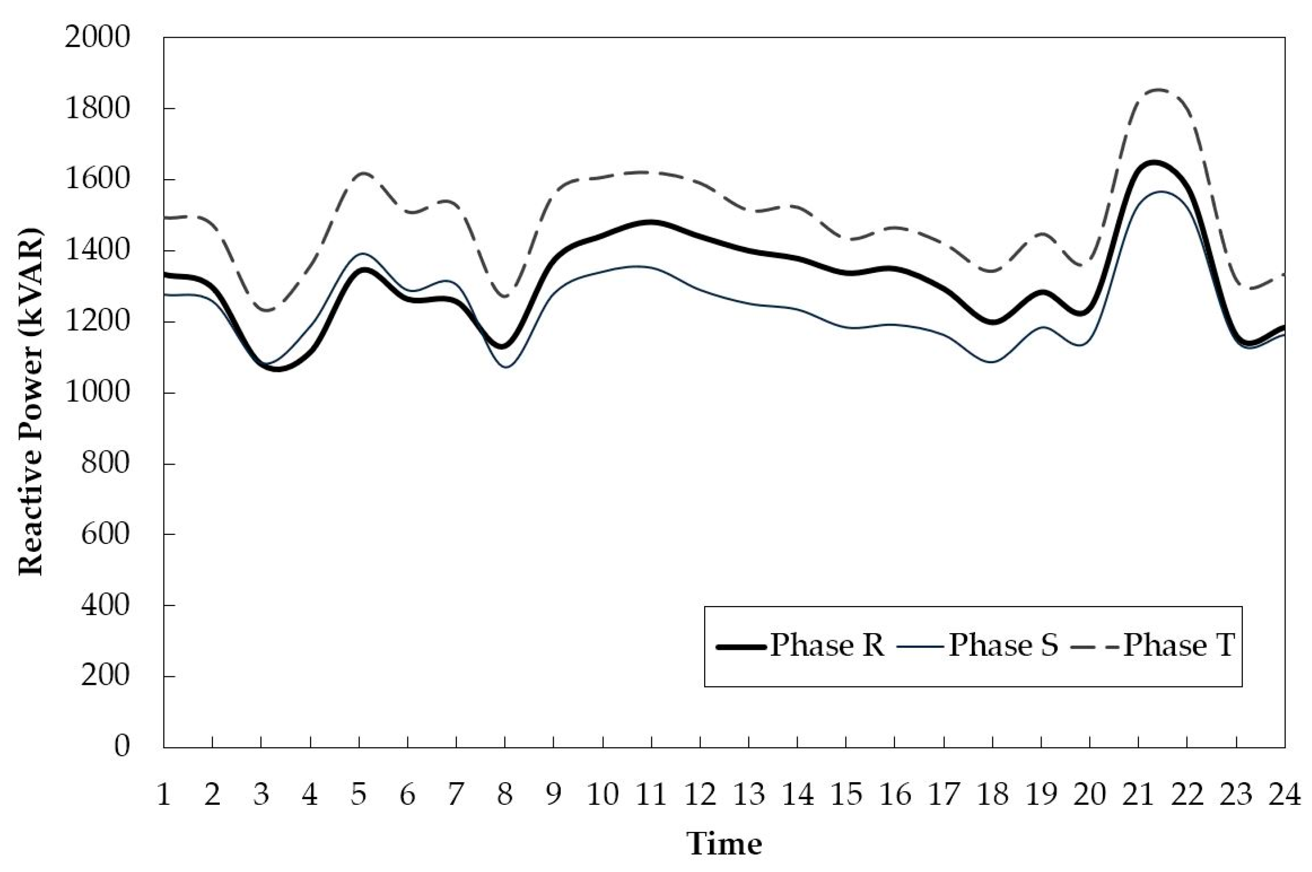
4. Simulation and Discussion
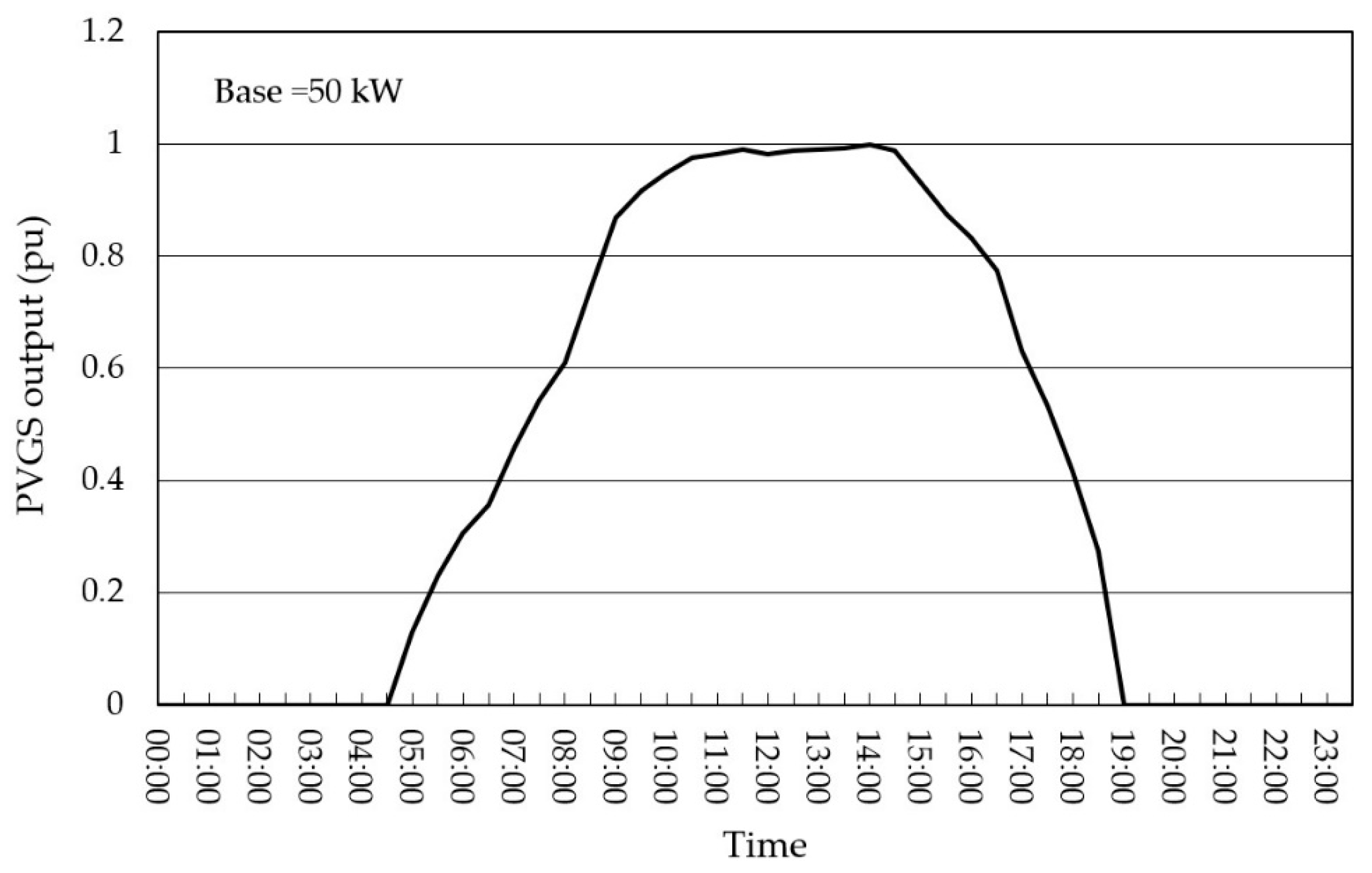
4.1. Generation Curve of PVGS
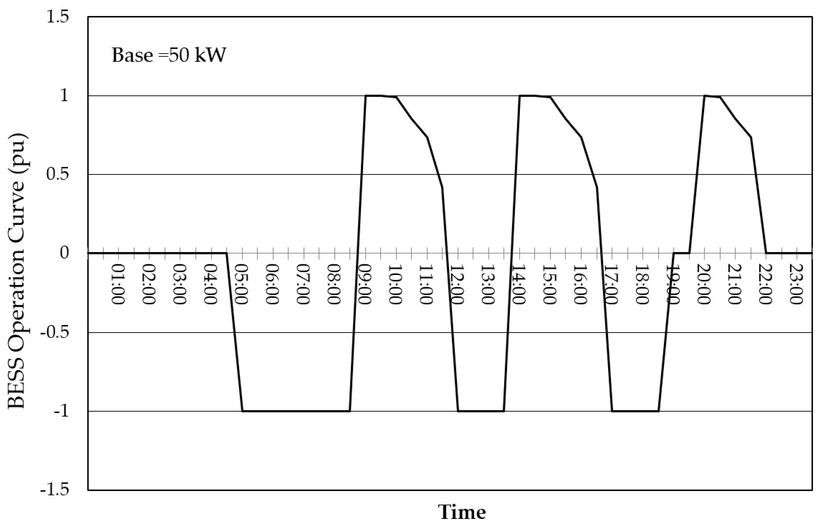
4.2. Operation Curve of the BESS
4.3. Optimal Sizing and Locating Combinations of the PVGS and BESS
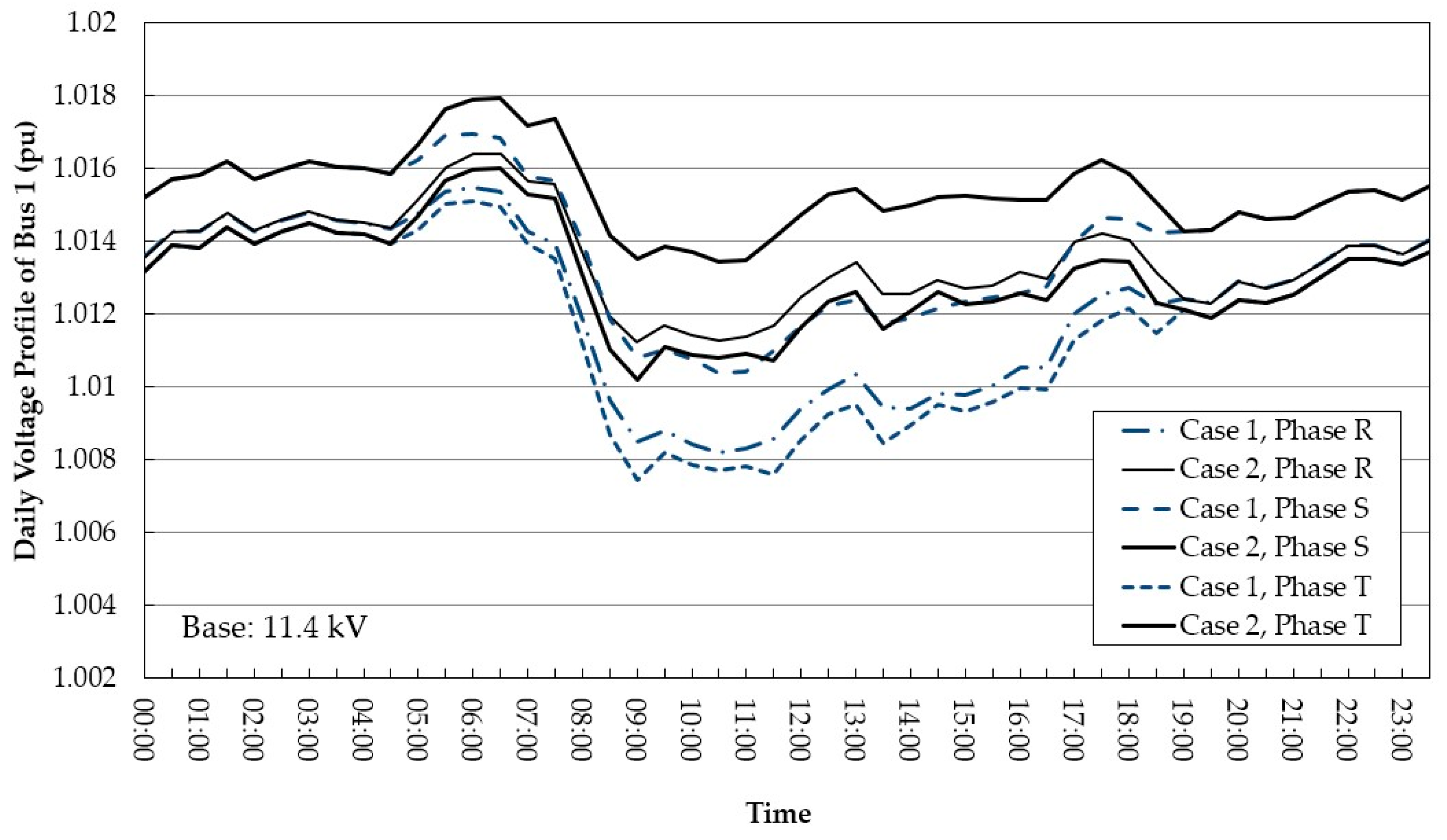
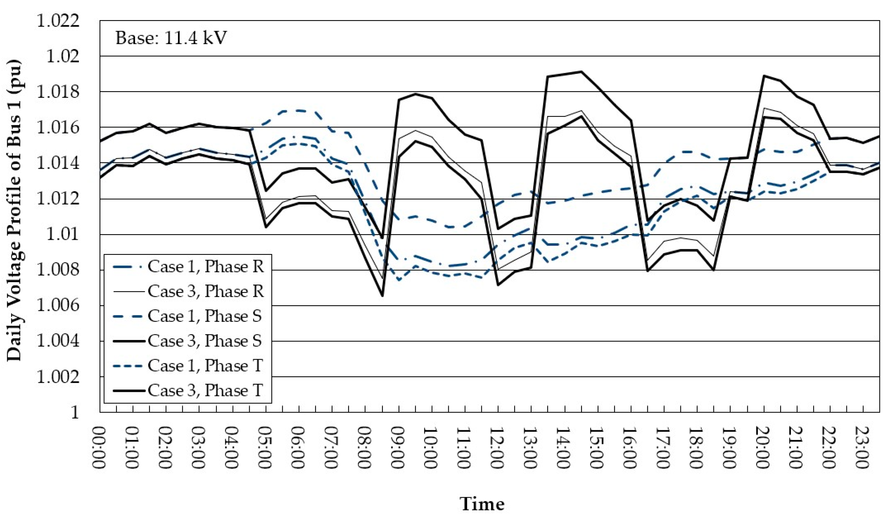
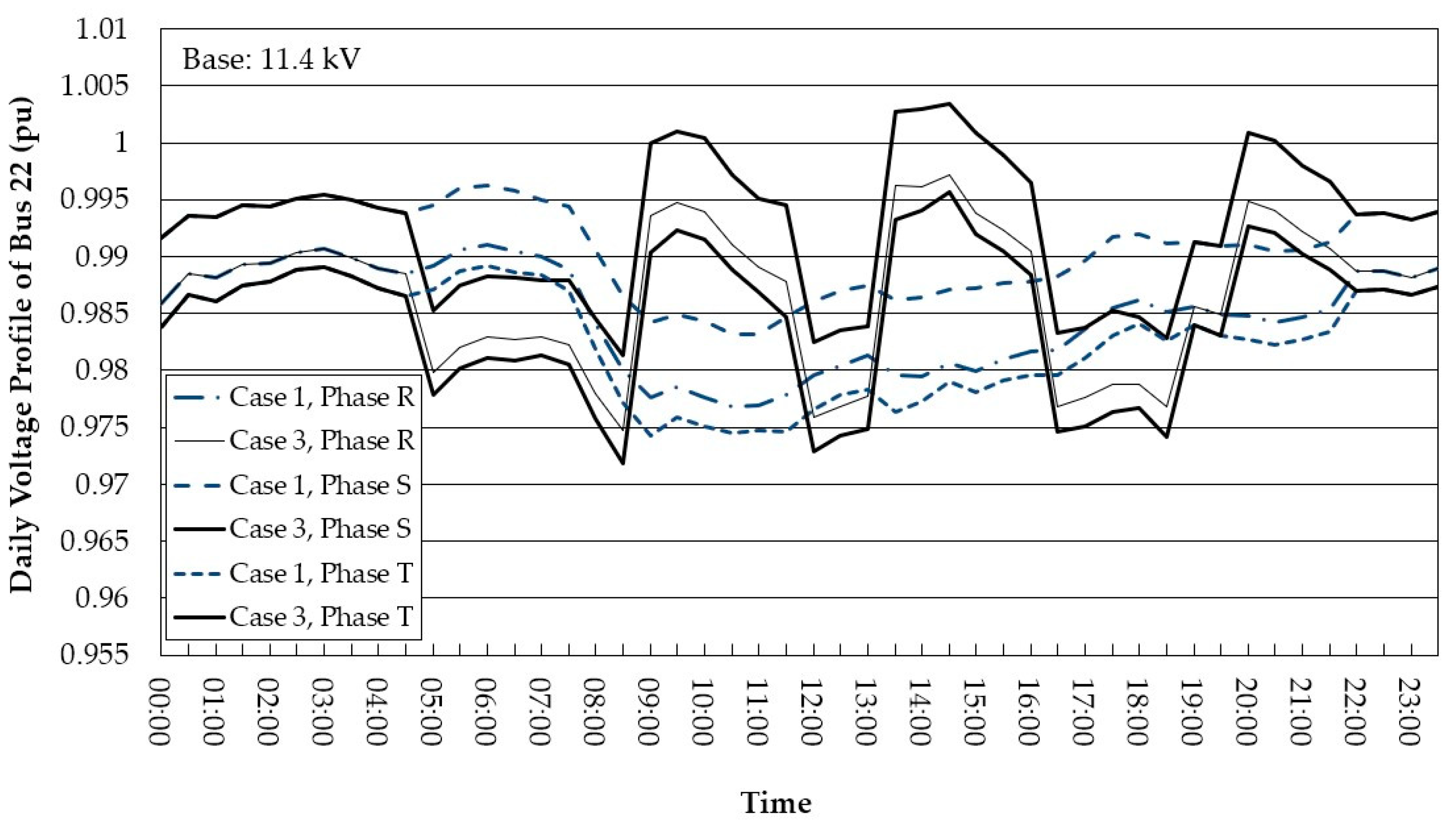
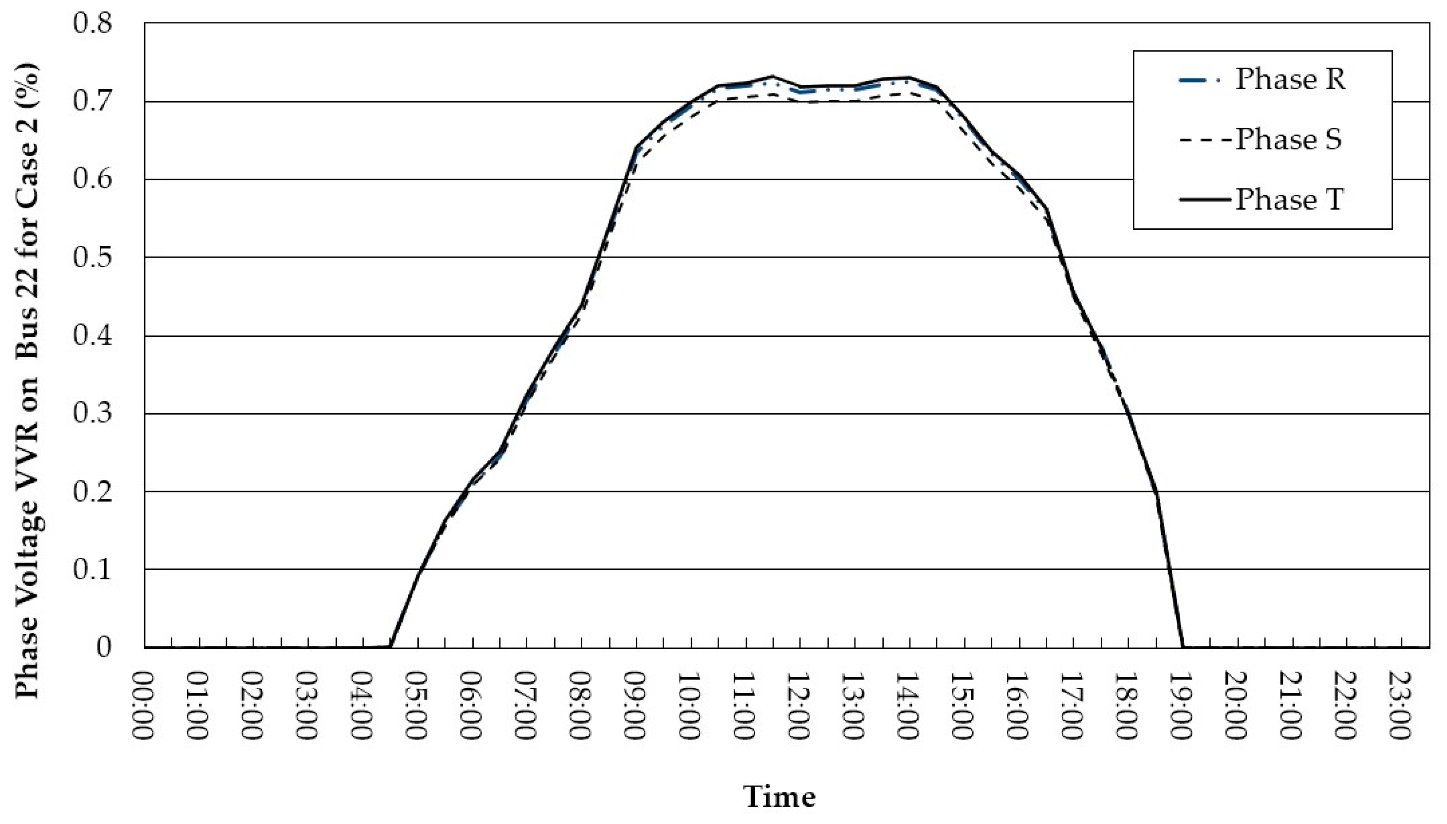
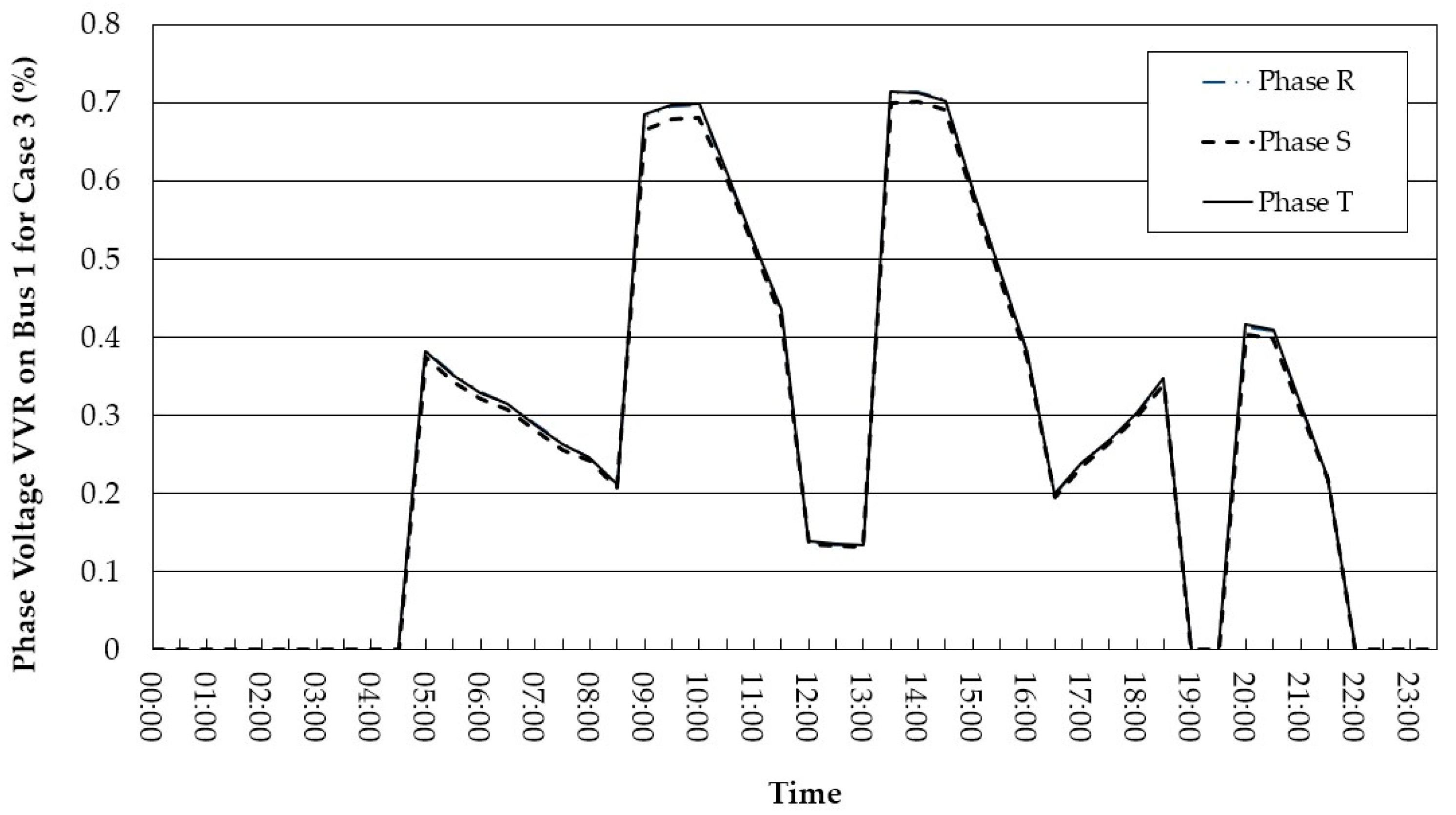
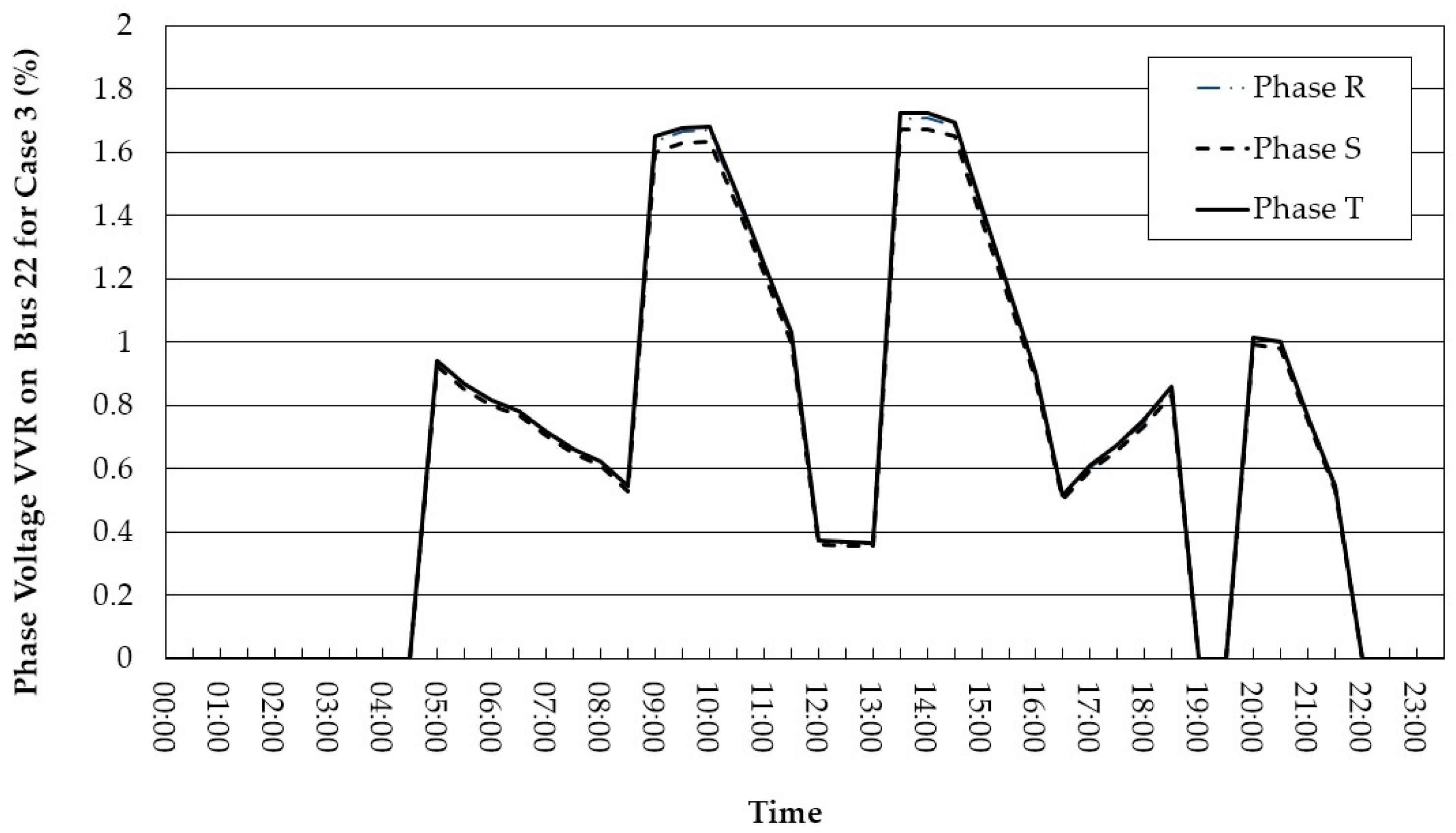
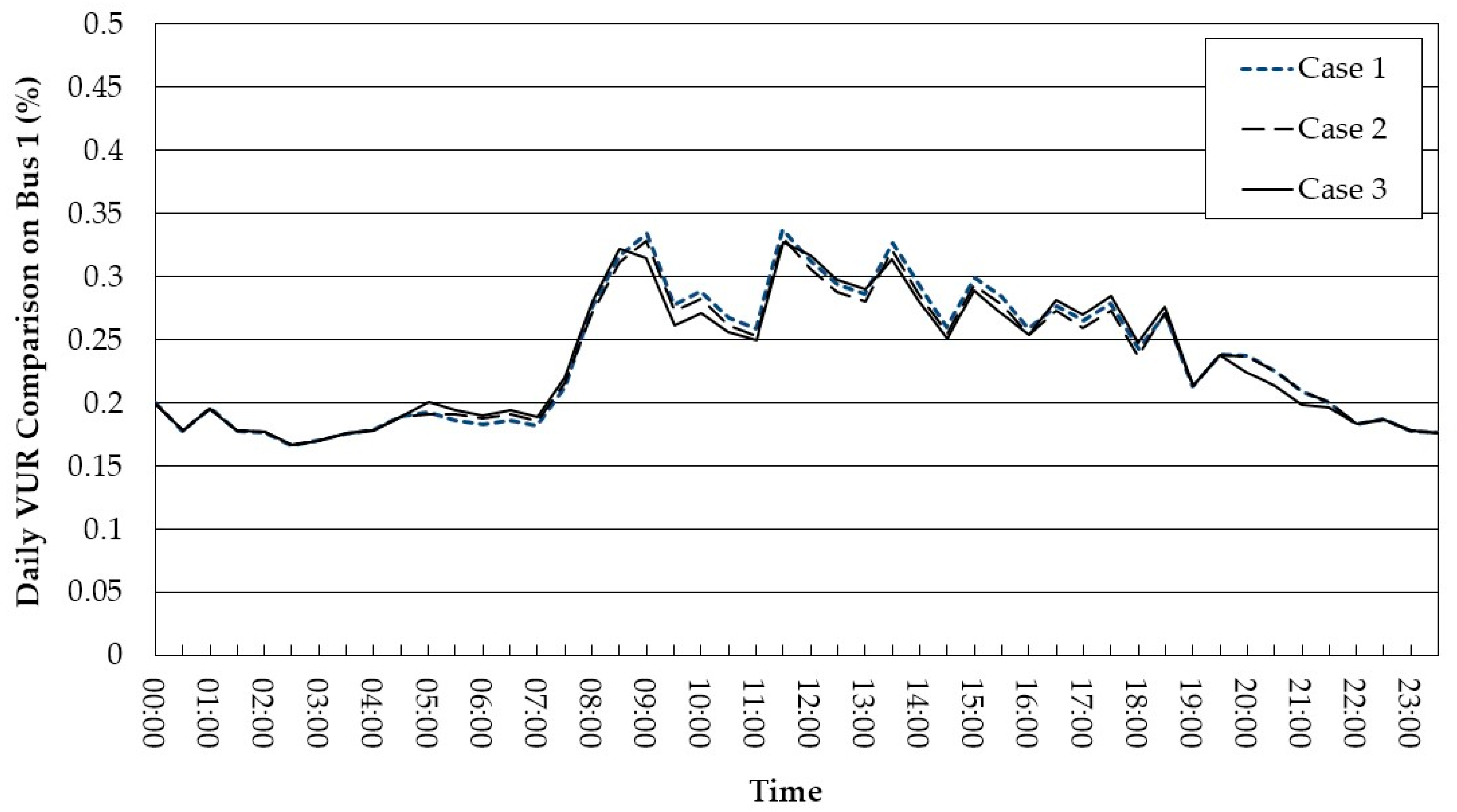
4.4. Analysis of the Voltage Variation Rate
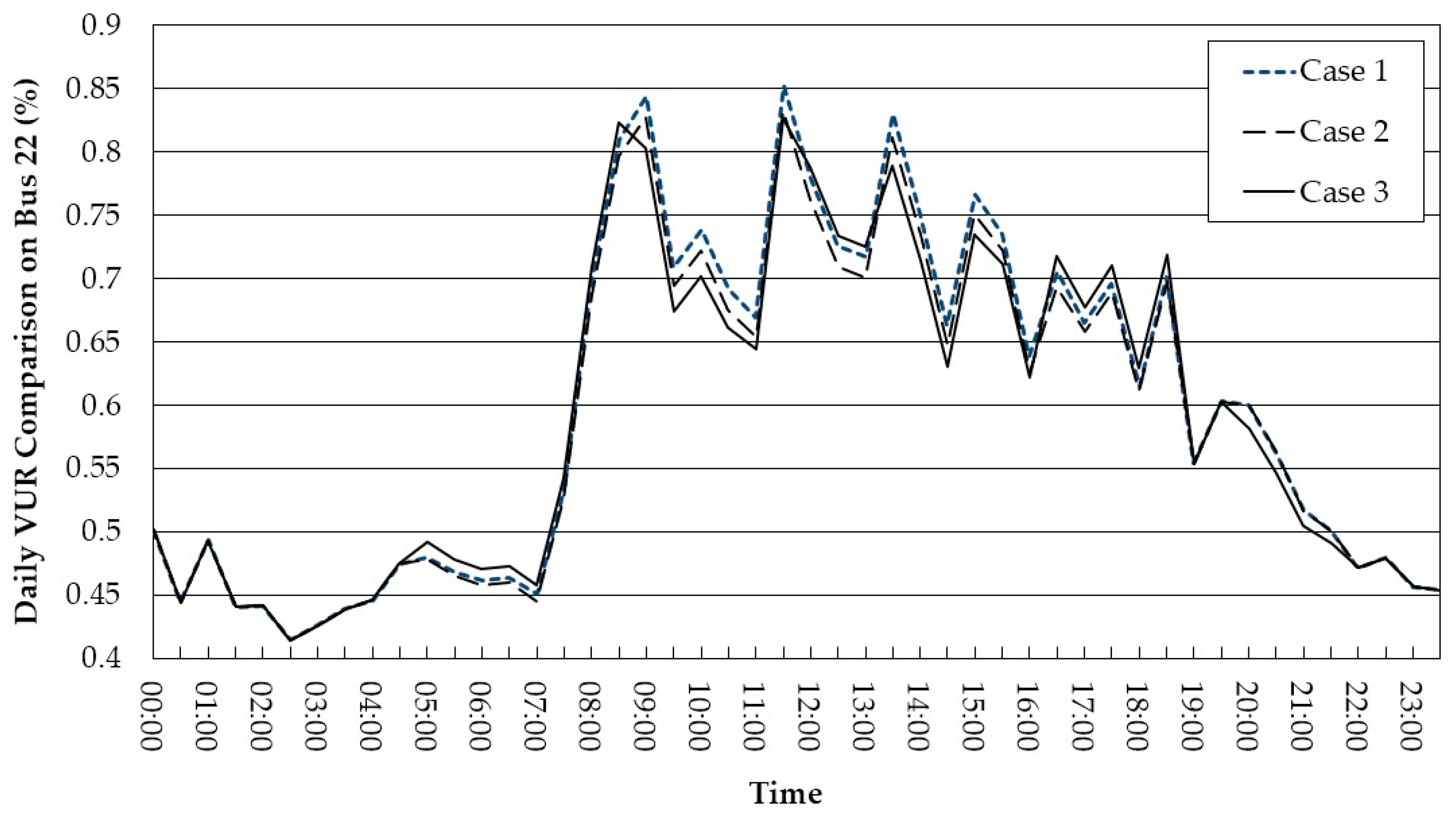
4.5. Analysis of the Voltage Unbalance Rate
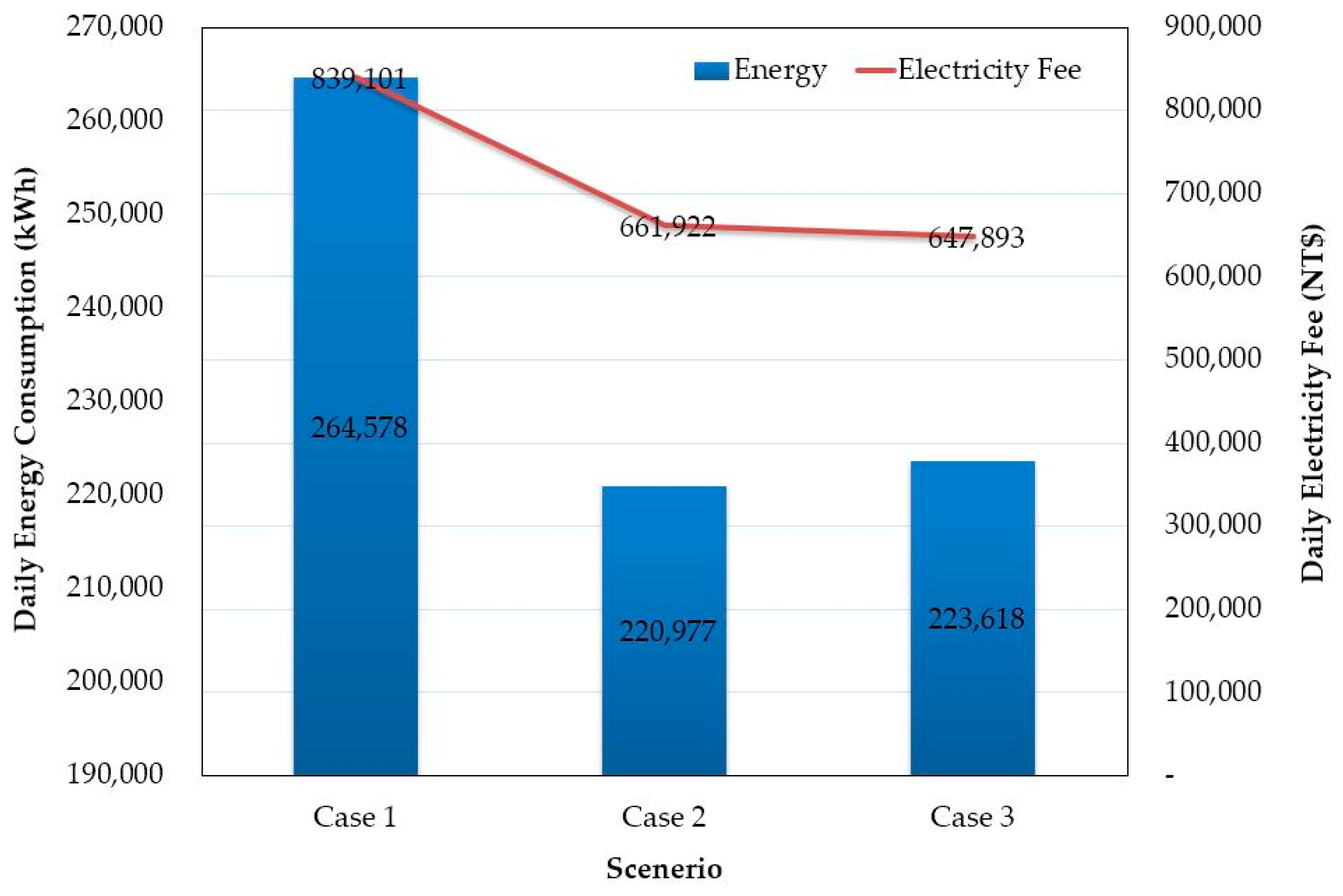
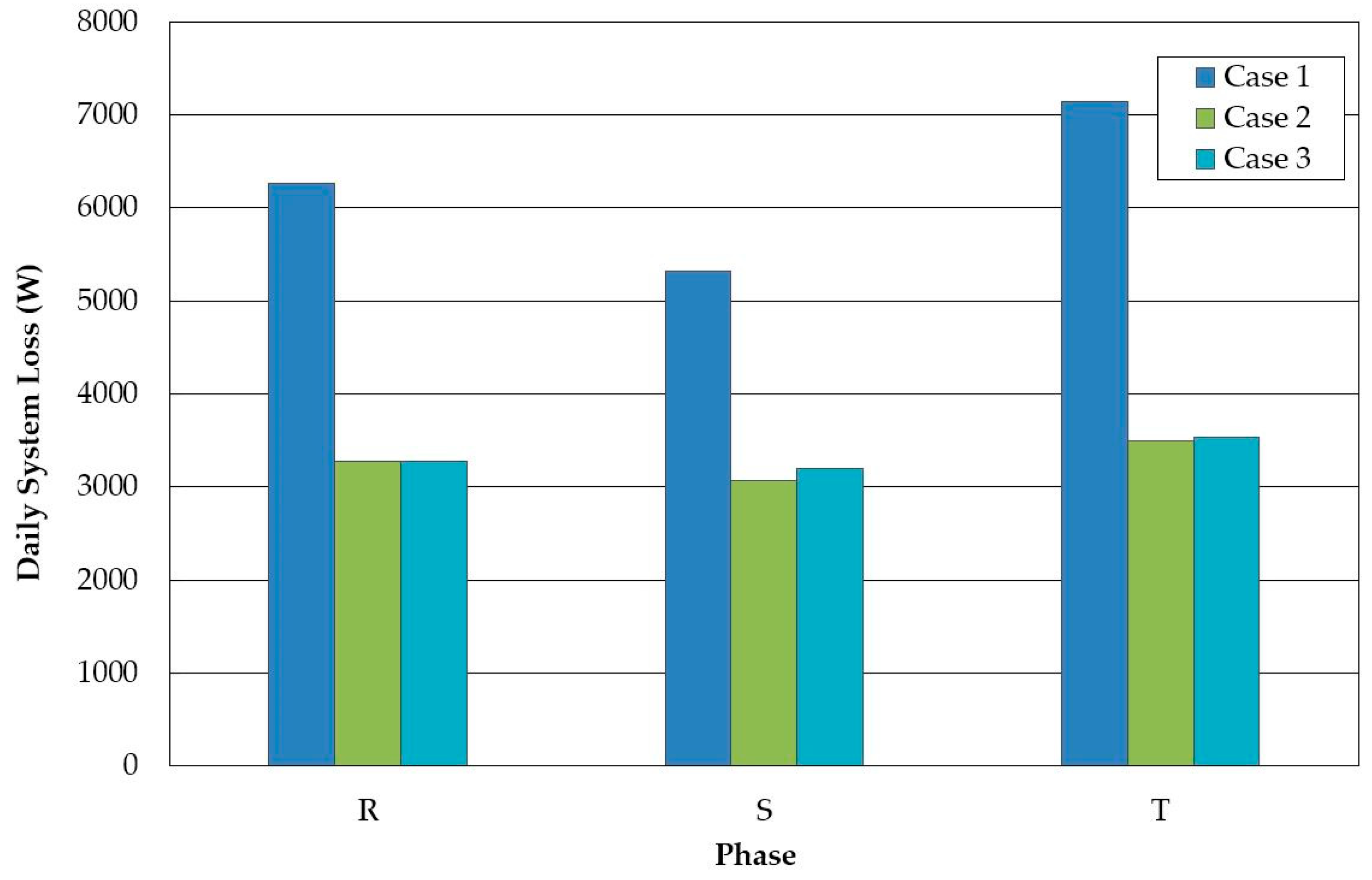
4.6. System Cost and System Loss
4.7. Convergence Performance of the RGA-ASCM
5. Conclusions
Author Contributions
Funding
Institutional Review Board Statement
Informed Consent Statement
Data Availability Statement
Acknowledgments
Conflicts of Interest
References
- Tsai, M.T.; Chen, S.L.; Wu, S.W.; Lin, C.P. The optimal placement of wing turbine in a distribution system. In Proceedings of the 2nd International Conference on Intelligent Technologies and Engineering Systems (ICITES 2013), Kaohsiung City, Taiwan, 2–14 December 2013. [Google Scholar]
- Zhang, Y.; Yao, F.; Iu, H.H.; Fernando, T.; Trinh, H. Operating optimization of wind-thermal systems considering emission problem. In Proceedings of the 40th Annual Conference of the IEEE Industrial Electronics Society, Dallas, TX, USA, 29 October 2014. [Google Scholar]
- Hakimi, S.M.; Moghaddas-Tafreshi, S.M. Optimal planning of a smart microgrid including demand response and intermittent renewable energy resources. IEEE Trans. Smart Grid 2014, 5, 2889–2900. [Google Scholar] [CrossRef]
- Grillo, S.; Marinelli, M.; Massucco, S.; Silvestro, F. Optimal management strategy of a battery-based storage system to improve renewable energy integration in distribution networks. IEEE Trans. Smart Grid 2012, 3, 950–958. [Google Scholar] [CrossRef]
- Olowu, T.O.; Sundararajan, A.; Moghaddamicisions, M.; Sarwat, A.I. Future challenges and mitigation methods for high photovoltaic penetration: A survey. Energies 2018, 11, 1782. [Google Scholar] [CrossRef]
- Sundararajan, A.; Olowu, T.O.; Wei, L.; Rahman, S.; Sarwat, A.I. Case study on the effects of the partial solar eclipse on distributed PV systems and management areas. IEEE Trans. Smart Grid 2019, 2, 477–490. [Google Scholar] [CrossRef]
- Debnath, A.; Olowu, T.O.; Parvez, I.; Sarwat, A. A binary search algorithm based optimal sizing of photovoltaic and energy storage systems. In Proceedings of the IEEE Green Technologies Conference (GreenTech), Virtual Conference, 7–9 April 2021. [Google Scholar] [CrossRef]
- Kaldellis, J.; Zafirakis, D.; Kondili, E. Optimum sizing of photovoltaic-energy storage systems for autonomous small islands. Int. J. Electr. Power Energy Syst. 2010, 32, 24–36. [Google Scholar] [CrossRef]
- Li, J. Optimal sizing of grid-connected photovoltaic battery systems for residential houses in Australia. Renew. Energy 2019, 136, 1245–1254. [Google Scholar] [CrossRef]
- Mohammed, A.Q.; Al-Anbarri, K.A.; Hannun, R.M. Optimal combination and sizing of a stand-alone hybrid energy system using a nomadic people optimizer. IEEE Access 2020, 8, 200518–200540. [Google Scholar] [CrossRef]
- Tutkun, N.; Çelebi, N.; Bozok, N. Optimum unit sizing of wind-PV-battery system components in a typical residential home. In Proceedings of the 2016 International Renewable and Sustainable Energy Conference (IRSEC), Marrakesh, Morocco, 14–17 November 2016. [Google Scholar]
- Nara, K.; Shiose, A.; Kitagawa, M.; Ishihara, T. Implement of genetic algorithm for distribution systems loss minimum re-configuration. IEEE Trans. Power Syst. 1992, 7, 1044–1051. [Google Scholar] [CrossRef]
- Park, J.B.; Park, Y.M.; Won, J.R.; Lee, K.Y. An improved genetic algorithm for generation expansion planning. IEEE Trans. Power Syst. 2000, 15, 916–922. [Google Scholar] [CrossRef] [Green Version]
- Fukuyama, Y.; Chiang, H.D. A parallel genetic algorithm for generation expansion planning. IEEE Trans. Power Syst. 1996, 11, 955–961. [Google Scholar] [CrossRef]
- Ciornei, I.; Kyriakides, E. A GA-API solution for the economic dispatch of generation in power system operation. IEEE Trans. Power Syst. 2012, 27, 233–242. [Google Scholar] [CrossRef]
- Park, Y.M.; Park, J.B.; Won, J.R. A hybrid genetic algorithm/dynamic programming approach to optimal long-term generation expansion planning. J. Electr. Power Energy Syst. 1998, 20, 295–303. [Google Scholar] [CrossRef]
- Chun, J.S.; Jung, H.K.; Hahn, S.Y. A study on comparison of optimization performances between immune algorithm and other heuristic algorithms. IEEE Trans. Magn. 1998, 34, 2972–2975. [Google Scholar] [CrossRef]
- Huang, S. An immune-based optimization method to capacaitor placement in a radial distribution system. IEEE Trans. Power Deliv. 2000, 15, 744–749. [Google Scholar] [CrossRef]
- Toma, N.; Endo, S.; Yamanda, K. Immune algorithm with immune network and MHC for adaptive problem solving. In Proceedings of the IEEE International Conference on Systems, Man, and Cybernetic, Tokyo, Japan, 12–15 October 1999. [Google Scholar]
- Kennedy, J.; Eberhart, R. Particle swarm optimization. In Proceedings of the IEEE International Conference on Neural Networks (ICNN’95), Perth, Australia, 27 November–1 December 1995. [Google Scholar]
- Eberhart, R.; Shi, Y. Comparing inertia weights and constriction factors in particle swarm optimization. In Proceedings of the Congress on Evolutionary Computation (CEC2000), La Jolla, CA, USA, 16–19 July 2000. [Google Scholar]
- Abido, M.A. Particle swarm optimization for multi-machine power system stabilizer design. In Proceedings of the IEEE Power Engineering Society Summer Meeting, Vancouver, BC, Canada, 15–19 July 2001. [Google Scholar]
- Meraihi, Y.; Gabis, A.B.; Mirjalili, S.; Ramdane-Cherif, A. Grasshopper optimization algorithm: Theory, variants, and applications. IEEE Access 2021, 9, 50001–50024. [Google Scholar] [CrossRef]
- Yang, X. Firefly algorithms for multimodal optimization. In Proceedings of the 5th International Symposium on Stochastic Algorithms (SAGA 2009), Sapporo, Japan, 26–28 October 2009. [Google Scholar]
- Niknam, T.; Golestaneh, F. Enhanced bee swarm optimization algorithm for dynamic economic dispatch. IEEE Syst. J. 2013, 7, 754–762. [Google Scholar] [CrossRef]
- Yang, X. A new metaheuristic bat-inspired algorithm. In Nature Inspired Cooperative Strategies for Optimization (NICSO 2010); González, J.R., Pelta, D.A., Cruz, C., Terrazas, G., Krasnogor, N., Eds.; Springer: Berlin/Heidelberg, Germany, 2010; Volume 284, pp. 65–74. [Google Scholar]
- Chen, S.L.; Zhan, T.S.; Tsay, M.T. Generation expansion planning of the utility with refined immune algorithm. Electr. Power Syst. Res. 2006, 76, 251–258. [Google Scholar] [CrossRef]
- Lin, W.M.; Cheng, F.S.; Tsay, M.S. Distribution feeder reconfiguration with refined genetic algorithm. IEE Proc.-Gener. Transm. Distrib. 2000, 147, 349–354. [Google Scholar] [CrossRef]
- Zhan, T.S.; Tsay, M.T. An improved genetic algorithm for the generation in electricity markets expansion planning of the utility in a competitive market. Int. J. Eng. Intell. Syst. 2004, 12, 167–173. [Google Scholar]
- Lin, W.M.; Zhan, T.S. Multiple-frequency three-phase load flow for harmonic analysis. IEEE Trans. Power Syst. 2004, 19, 897–904. [Google Scholar] [CrossRef]
- Lin, W.M.; Teng, J.H. Three-phase distribution network fast-decoupled power flow solution. Int. J. Electr. Power Energy Syst. 2000, 22, 375–380. [Google Scholar] [CrossRef]
- Hou, J.C. Optimal Injection-Point Decision of the Photovoltaic Generation with Energy Storage System. Master’s Thesis, Kao Yuan University, Kaohsiung City, China, 2019. [Google Scholar]


| Bus | 3 | 4 | 5 | 6 | 7 | 8 | 9 | 10 | |
| PVGSCapacity(kW) | Case 2 | 0 | 250 | 0 | 600 | 0 | 0 | 0 | 0 |
| Case 3 | 400 | 250 | 0 | 250 | 0 | 0 | 0 | 0 | |
| Bus | 11 | 12 | 13 | 14 | 15 | 16 | 17 | 18 | |
| PVGSCapacity(kW) | Case 2 | 0 | 0 | 0 | 0 | 600 | 0 | 250 | 0 |
| Case 3 | 0 | 0 | 250 | 0 | 400 | 500 | 250 | 0 | |
| Bus | 19 | 20 | 21 | 22 | 23 | 24 | 25 | 26 | |
| PVGSCapacity(kW) | Case 2 | 750 | 0 | 0 | 500 | 0 | 0 | 400 | 0 |
| Case 3 | 250 | 250 | 0 | 100 | 350 | 0 | 300 | 0 | |
| Bus | 27 | 28 | 29 | 30 | 31 | 32 | Total Cap. | ||
| PVGSCapacity(kW) | Case 2 | 350 | 0 | 400 | 0 | 400 | 0 | 4500 | |
| Case 3 | 250 | 0 | 250 | 0 | 250 | 0 | 4300 | ||
| Bus | 3 | 4 | 5 | 6 | 7 | 8 | 9 | 10 | |
| BESS Capacity (kW) | Case 3 | 350 | 200 | 0 | 200 | 0 | 0 | 0 | 0 |
| Bus | 11 | 12 | 13 | 14 | 15 | 16 | 17 | 18 | |
| BESS Capacity (kW) | Case 3 | 150 | 0 | 100 | 0 | 300 | 300 | 200 | 0 |
| Bus | 19 | 20 | 21 | 22 | 23 | 24 | 25 | 26 | |
| BESS Capacity (kW) | Case 3 | 200 | 200 | 0 | 100 | 300 | 0 | 250 | 0 |
| Bus | 27 | 28 | 29 | 30 | 31 | 32 | Total Cap. | ||
| BESS Capacity (kW) | Case 3 | 250 | 0 | 250 | 200 | 250 | 0 | 3800 | |
| Case | Algorithm | Total PVGS Installation Capacity (kW) | Total BESS Installation Capacity (kW) | Total Installation Investment Cost (NT$) |
|---|---|---|---|---|
| 2 | SGA | 4950 | -- | 345,600,000 |
| IA | 5300 | -- | 371,000,000 | |
| RGA-ASCM | 4500 | -- | 315,000,000 | |
| 3 | SGA | 4650 | 3950 | 538,800,000 |
| IA | 4800 | 4050 | 554,700,000 | |
| RGA-ASCM | 4300 | 3800 | 506,200,000 |
| Section Name | Time Section | Price |
|---|---|---|
| peak | AM 10:00–PM 12:00$$PM 01:00–PM 05:00 | NT $4.61/kWh |
| half-peak | AM 07:30–AM 10:00$$PM 12:00–PM 01:00 | NT $2.87/kWh |
| off-peak | AM 00:00–AM 07:30$$PM 10:30–AM 00:00 | NT $1.29/kWh |
Publisher’s Note: MDPI stays neutral with regard to jurisdictional claims in published maps and institutional affiliations. |
© 2022 by the authors. Licensee MDPI, Basel, Switzerland. This article is an open access article distributed under the terms and conditions of the Creative Commons Attribution (CC BY) license (https://creativecommons.org/licenses/by/4.0/).
Share and Cite
Chiang, M.-Y.; Huang, S.-C.; Hsiao, T.-C.; Zhan, T.-S.; Hou, J.-C. Optimal Sizing and Location of Photovoltaic Generation and Energy Storage Systems in an Unbalanced Distribution System. Energies 2022, 15, 6682. https://doi.org/10.3390/en15186682
Chiang M-Y, Huang S-C, Hsiao T-C, Zhan T-S, Hou J-C. Optimal Sizing and Location of Photovoltaic Generation and Energy Storage Systems in an Unbalanced Distribution System. Energies. 2022; 15(18):6682. https://doi.org/10.3390/en15186682
Chicago/Turabian StyleChiang, Ming-Yuan, Shyh-Chour Huang, Te-Ching Hsiao, Tung-Sheng Zhan, and Ju-Chen Hou. 2022. "Optimal Sizing and Location of Photovoltaic Generation and Energy Storage Systems in an Unbalanced Distribution System" Energies 15, no. 18: 6682. https://doi.org/10.3390/en15186682
APA StyleChiang, M.-Y., Huang, S.-C., Hsiao, T.-C., Zhan, T.-S., & Hou, J.-C. (2022). Optimal Sizing and Location of Photovoltaic Generation and Energy Storage Systems in an Unbalanced Distribution System. Energies, 15(18), 6682. https://doi.org/10.3390/en15186682