Predicting Vehicle Refuelling Trips through Generalised Poisson Modelling

Highlights

What are the main findings of this paper?

• The GP-1 model developed is statistically significant, and can be used to model future refuelling trends.
• Prediction of refuelling trip counts considering weather patterns and day of the month.

What is the implication of the main finding?

• Awareness of the refuelling behaviours of alternative fuel vehicles such as hydrogen vehicles when such data becomes available.
• Informing infrastructure requirements for refuelling.

Abstract

This paper presents a model to predict the number of refuelling trips by vehicles on any given day considering weather conditions and time of the year. The predicted refuelling trips were founded on count-based data, i.e., data that contain events that occur at a certain rate. The paper presents an algorithm developed using Python programming language and the statsmodels module to achieve this. The results indicate that the GP-1 model developed in this paper is statistically significant at the 95% confidence level as it was able to converge—however, precipitation and high ambient temperature conditions are considered statistically insignificant in this model. The viability of the model was further tested on the remaining 20% of the data. Sensitivity tests indicate that there is a good correlation between the actual trips and predicted trips when 70% of the data are used to train the model. Overall, the model presented can be used to predict the number of trips taken by vehicles to refuel as well as model future trends, accurately. This model, can in the future, be applied to predict the refuelling behaviour of alternative fuel vehicles such as hydrogen fuel vehicles, when such data become available.

1. Introduction

The challenges of climate change, energy security and urban air pollution have piqued interest in alternative fuel vehicles such as hydrogen fuel vehicles (HFVs). The use of HFVs in the near future forms part of social, environmental and economic goals, worldwide [1]. Countries such as the United States of America, Japan, and many European nations have introduced HFVs onto their roads due to the associated benefits [2]. South Africa, where the transport sector contributes to about 60 metric tons of carbon dioxide equivalent emitted annually (a similar scale to emissions from industrial operations), also benefits from adopting these vehicles [3]. The country has a vested interest in integrating renewable energy sources as per its Integrated Resource Plan 2019, and hydrogen is seen to become a game-changer in the country’s aspirations to move towards a net-zero carbon economy. In fact, it is the goal of South Africa’s Hydrogen Society Roadmap to decarbonise heavy-duty transportation by the year 2050 [4].

The use of hydrogen as an alternative source of energy is highly motivated within the South African transport sector. However, for HFVs to prove competitive against conventional modes of transport, there must be well-built, accessible refuelling infrastructure available, and currently, this is scarce [5,6]. Ref. [6] indicates that HFVs and refuelling infrastructure are complementary goods and both must successfully penetrate the transportation market for either to be successful. Studies such as [7] indicate that a major success determinant in the adoption of these vehicles is the availability of hydrogen-based infrastructure that comprises important components and facilities to sufficiently support the hydrogen fuel demand of HFVs [7]. In Ref. [8], it is further noted that a hydrogen refuelling network is necessary for HFVs to operate; in fact, the study states that these vehicles will be unable to operate and their commercial deployment limited if such networks are not established. For substantial market penetration of HFVs within the transport sector, the introduction of commercial hydrogen vehicles and the network of fuelling stations to supply them with hydrogen needs to occur simultaneously [9].

Essentially studying the refuelling behaviour of conventional vehicle drivers could offer useful information to model hydrogen refuelling infrastructure networks, once such data are available. In turn, it could also provide statistical models to evaluate fuel consumption for enhancing economic efficiency. Comprehending how far people travel and how many trips people take within a specific region can also tremendously help in infrastructure planning. Studies such as [1,10] show that fuel consumption patterns are influenced by factors such as weather conditions, among others. Several studies are focusing on the refuelling behaviour of conventional vehicles, hybrid ICE, battery-electric and HFVs [7,11,12,13]; however, very limited studies consider the stochastic nature of refuelling, and most do not consider the impacts of weather. Furthermore, the majority of these studies focus on conventional vehicles and electric vehicles. For example, [14] studies the relationship between electric vehicle adoption and consumer behaviour; [15] looks at the energy costs and refuelling behaviour through the use of Monte Carlo simulations on electric vehicles. Although there are studies, such as [16], that consider the stochastic nature of refuelling behaviour, it does not take into account the impact of weather conditions on driving trips and consequently refuelling behaviour, especially since weather conditions are shown to have an impact on fuel economy, with users seeing more fuel consumption during colder days than warmer ones [1,10].

Most studies make use of scenario-based modelling, MARKAL models, agent-based modelling and system dynamics about alternative fuel vehicle (AFV) refuelling infrastructure [9,14,17,18], and these models are limited in its ability to study the stochastic nature of refuelling behaviour.

Ultimately, developing a model that can predict the amount of refuelling trips a vehicle will make based on any day in the year, the temperature and precipitation on that day can prove useful to countries looking to adopt alternative fuel vehicles such as HFVs in the future. Although this model uses general vehicle data, it will still allow analogies between cities of the same size to be drawn, and as such, help to predict the future trip counts and trends expected for HFVs once adoption escalates. For this paper, a slightly modified approach is used—where the Poisson probability distribution is modified to handle over- and under-dispersion. This is also known as GP-1 (generalised Poisson regression model 1). The Negative Binomial Model (NBM) and generalised Poisson regression model 2 was also considered [19,20]. However, it was noted that these models do not actually converge for similar data sets.

Hence, this paper presents a Poisson prediction model to predict the number of trip counts to advise refuelling behaviour in any region or city, and for any vehicle type, should the relevant data be available. The model allows the prediction of refuelling trip counts, based on the assumption that a vehicle would most likely need to refuel when travelling for 320 km. Thus, these data will then be used to extract driving trends of current general vehicles that can then be used as an analogy for HFV refuelling behaviour. Features that were used to assist the model predict the trip counts include temperature, precipitation, and day of month, as sourced in Ref. [21].

The novelty of this study lies in the fact that this model can provide useful insights and trends on the expected trips taken by drivers (on any given day of the year and in any weather condition) and consequently expected demand for fuel from refuelling stations. This type of model is ideal for count-based data where the rate of occurrence changes over time from one observation to the next such as in the case of refuelling behaviour.

Compared to conventional fuel (gas, diesel etc.), hydrogen used for transport is still relatively small, with only a countable number of dispensaries distributed over large geographical areas in countries where HFVs have been introduced commercially [22,23]. In countries where HFVs are still being introduced, there are few to no such facilities present. In fact, several papers have established the impact of adequate refuelling stations/infrastructure on the adoption/penetration of HFVs [24,25,26,27,28,29]. This paper proposes a model to predict or ‘count’ the number of refuelling trips taken by a vehicle user considering factors such as temperature, precipitation, and day of the month (time of year). Unlike other papers that only consider the travel time to a refuelling station [16], the novelty of the proposed model is the capability to predict how many times a vehicle would travel a typical distance to fuel up within certain weather conditions for any given day in the year. The proposed model integrates complex Poisson modelling and will be implemented through an algorithm. Although various modelling methodologies such as the hidden Markov model and Monte Carlo simulations were reviewed and considered, this approach was considered the most suitable in terms of the nature of the model prediction required as counts are used as input data. Another possible model considered was the Markov model which has been used for the prediction of driver and refuelling behaviour in several studies [30]. However, this paper preferred the use of the Poisson regression model to predict future data as it allows for more complexity when compared to the Markov approach.

This paper’s contributions include:

• Adaption and testing of an algorithm for predicting driving trip to advise the refuelling behaviour.
• Prediction of refuelling trips or trip counts considering weather patterns and day of the month.

2. Methodology

The regression model aims to predict the number of trips counts for refuelling on any given day, and in any weather condition, by using a set of regression variables from the data gathered, namely, day, day of the week, month, high temperature, low temperature, and precipitation to ‘explain’ the variance in the observed trip counts. The data set used to set up this model comes from the New York Count (NYC) open database where the count for trips by distance (only driving data/trips) in NYC county, specifically for the year 2019 is considered. Data are required to develop this model and the NYC database was used since it is readily available and vaster compared to the data available on the South African trip counts. It should be understood that, if such data become available in South Africa, then these data will be used in the prediction model and the South African situation analysed.

The methodology followed to prove the model and accuracy of the outputs obtained is detailed in Section 2.1 and Section 2.2 below.

2.1. Generalised Poisson Regression Modelling

A Poisson regression model is a form of linear regression analysis used to model and predict count-based data. This model assumes the response variable Y has a Poisson distribution, a discrete probability distribution, that expresses the probability of a given number of events occurring at a fixed time interval. It also assumes the logarithm of its expected value can be modelled by a linear combination of parameters. In doing so, it is necessary to investigate which of these parameters has a significant effect on the response variable Y. That is, which X-values will work with the Y-value. It is also used for unique events and thus uses the Poisson distribution:

$$P\left(Y=y\right)=\frac{e^{-\lambda }{\lambda }^y}{y!} for y=0,1,\dots ,\infty$$

(1)

In general, it is a good idea to use the Poisson model for count-based data sets as it has the following properties [30]:

• It is made up of a sequence of random variables.
• It is a stochastic process, as each time the Poisson process is run it will produce a different sequence of random outcomes as per the probability distribution.
• It is a discrete process.

The Probability Mass Function (PMF) distribution is given as follows:

$$P_x\left(k\right)=\frac{e^{-\left(\lambda t\right)}\times {\left(\lambda t\right)}^k}{k!}=Poisson \left(\lambda t\right)$$

(2)

where $P_x\left(k\right)$ is the probability of seeing k events in time t, lambda ($\lambda$), is the event rate, and k is the number of events. So, the expected value (mean) for a Poisson distribution is $\lambda$. Based on Equation (2), one would expect to see $\lambda$. in any unit time interval, i.e., $\lambda \times t$. However, since $\lambda$ is not constant, a simple mean model for predicting the future counts of events cannot be used as λ changes from one observation to the next. Hence it is assumed that $\lambda$ is influenced by a vector regression of variables (regressors). In this study, this will be referred to as the matrix of regression variables, X. It should be noted that the function of the regression model is to fit the observed counts, y, to the matrix, X.

The data available include data on dates, high and low temperatures, as well as precipitation. Furthermore, data on the month and day of the month were derived from the ‘date’ data obtained. The observed counts, y, are fit to the matrix, X, by fixing values of the vector to the regression coefficient, Beta ($\beta$). To connect the matrix, X, to $\beta$, a link function where the exponential link function works well was used. This link function allows $\lambda$ to remain non-negative even when X or $\beta$. have negative values. Hence, the probability of observing a count y_i for the specification for ‘ith’ count, corresponding to the regression row $x_i$ is distributed as per the following PMF

$$PM{F}_{\left(y_i|x_i\right)}=\frac{e^{-{\lambda }_i}\times {\lambda }_i^{y_i}}{y_i!}$$

(3)

where $PMF$ is the probability of seeing count $y_i$ given the regression vector, $x_i$, and $\lambda$ event rate for the ith sample.

The exponential link function equation is shown as follows:

$${\lambda }_i=e^{x_i\beta }$$

(4)

where ${\lambda }_i$ is the event rate for the ith sample, $x_i$, is the regressor for the ith sample, and $\beta$ is the regression coefficients vector. Once the developed model is fully trained, the beta coefficients will be known, and the model will then make predictions using the following equation:

$$y_p={\lambda }_p=e^{x_p\beta }$$

(5)

where $y_p$ refers to the predicted count, is the predicted event rate for the pth sample, and $x_p$ is the regressor for the pth sample.

2.2. Data

The data required to develop the prediction model and train the algorithm were obtained from the United States Department of Transportation (Bureau of Transportation Statistics) [31].

To develop this model, the following data were used:

• Trips by distance in the year 2019 in NYC.
• Weather conditions in the same period (data obtained from [21]).

A sample of the trip counts data used to set up this prediction model are shown in Table 1.

Table 1. Sample trip count data used in the prediction model.

Level	Date	State FIPS *	State Postal Code	County FIPS	County Name	Trips
County	1 January 2019	36	NY	36,061	New York County	23,921
County	2 January 2019	36	NY	36,061	New York County	20,922
County	3 January 2019	36	NY	36,061	New York County	19,167
County	4 January 2019	36	NY	36,061	New York County	20,500

* FIPS—Federal Information Processing Standards.

A sample of the weather data used in this prediction model are shown in Table 2.

Table 2. Sample weather data used in the prediction model.

Time	Temp High (°C)	Temp Low (°C)	Precipitation (mm)
1 January	15.6	5.6	35.3
2 January	5	1.7	0.0
3 January	7.2	3.9	0.0
4 January	8.3	2.8	0.0
5 January	8.3	5.6	5.8

In order to derive the relationship between weather conditions (temperature and precipitation) and the trip counts, the two data sets presented in Table 1 and Table 2 were combined. This is as shown in Table 3.

Table 3. Sample of combined data.

Date	Temp High (°C)	Temp Low (°C)	Precipitation (mm)	Trip Count
1 January 2019	15.6	5.6	34.75	23,921
2 January 2019	5	1.7	0	20,922
3 January 2019	7.2	3.9	0	19,167
4 January 2019	8.3	2.8	0	20,500

2.3. Assumptions and Limitations

2.3.1. Assumptions

The following model requirements and assumptions were considered in this paper:

• Y- values must be counts.
• Counts must be whole positive numbers as the Poisson distribution is discrete.
• Counts should follow Poisson distribution such that the variance is equal to the mean.
• Explanatory variables must be continuous, dichotomous or ordinal.
• Observations must be independent.
• Since $\lambda$ is not a constant, a simple mean model for predicting the future counts of events cannot be used as $\lambda$ changes from one observation to the next. Hence it is assumed that $\lambda$ is influenced by a vector regression of variables (regressors).
• The model is rooted in the assumption that the variance is equal to the mean as the variable y is a random variable that follows the Poisson distribution whose variance equals the mean.

2.3.2. Limitations

The Poisson model is not able to explain variability in observed counts due to the assumption that the variance is equal to the mean, i.e., the model makes an assumption that the counts need to be equally dispersed. In most datasets, there is over-dispersion (variance > mean), for example, the variance for y would be greater than the model prediction. Similarly, there is also under-dispersion (variance < mean). The effect, in the end, is that the model will not be able to predict changes in the observations. To resolve this issue, it is assumed that the variance is a function of the mean:

$$Variance=mean+\alpha \times mea{n}^p$$

(6)

where alpha ($\alpha$) is known as the dispersion parameter which accounts for additional variability for the regression model.

• $\alpha$ = 0—The standard Poisson model assumption.
• $\alpha$ > 0 and p = 1 and p = 2—A new model called the Negative Binomial (NB) regression model which works well for real-world data [30].

The GP-1 model assumes that y is a random variable with the following distribution:

$$P_y\left(y=k\right)=\frac{e^{-\left(\lambda +\alpha \times k\right)}\times {\left(\lambda +\alpha \times k\right)}^{k-1}}{k!}$$

(7)

$$Mean\left(y\right)=\frac{\lambda }{1-\alpha }$$

(8)

$$Variance\left(y\right)=\frac{\lambda }{{\left(1-\alpha \right)}^3}$$

(9)

The dispersion parameter, $\alpha$, is then determined from Equation (9):

$$\alpha =\frac{{{\displaystyle \sum }}_{i=1}^N\left(\frac{\left|y_i-{\widehat{y}}_i\right|}{\sqrt{\widehat{y_i}}}-1\right)\times \widehat{(y_i}{)}^{\left(1-p\right)}}{N-k-1}$$

(10)

where N is the number of training samples, k is the number of regression variables, $y_i$, the ith observed value, ${\widehat{y}}_i$, the predicted Poisson rate, ${\lambda }_i$, corresponding to the ith training sample, and p = 1 or 2 for a GP1 or a GP2 model.

2.4. Goodness of Fit

Goodness of fit (GOF) describes how well a statistical model fits into a set of observations [32], that is, indicates whether the observed data align with what is expected. In this study, the developed prediction model will make use of the chi-square test to test whether a relationship exists between categorical variables, as well as to determine whether the sample represents the whole. Using the chi-square goodness of fit test allows a conclusion on whether the sample data are likely to be from the specified theoretical distribution which is to be specified, i.e., does the set of data values match the predicted distribution profile expected? [32]. Additionally, the chi-square test can be used for discrete distributions and the Poisson distributions hence thought to be the best test for the purposes of this study.

2.5. Training Algorithm

To train the Poisson regression model, $\beta$, values need to be obtained. This would make the vector y probable. The Maximum Likelihood Estimation (MLE) method is the approach used to obtain the required $\beta$ coefficients. This is derived from the log-likelihood function until the equation in terms of $\beta$ is obtained:

$${{\displaystyle \sum }}_{i=1}^n\left(y_i-e^{x_i\beta }\right)x_i=0$$

(11)

Solving this equation for $\beta$-values will obtain the MLE for $\beta$.

A package was used to train the algorithm for the Poisson regression modelling. For this paper, the order of the process followed is as follows:

• Training the regression model on training data.
• Test the performance of the model on test data and compare them with actual counts to understand how well the model has performed.
• Perform a ‘goodness-of-fit’ measure to check how well the model has been trained.

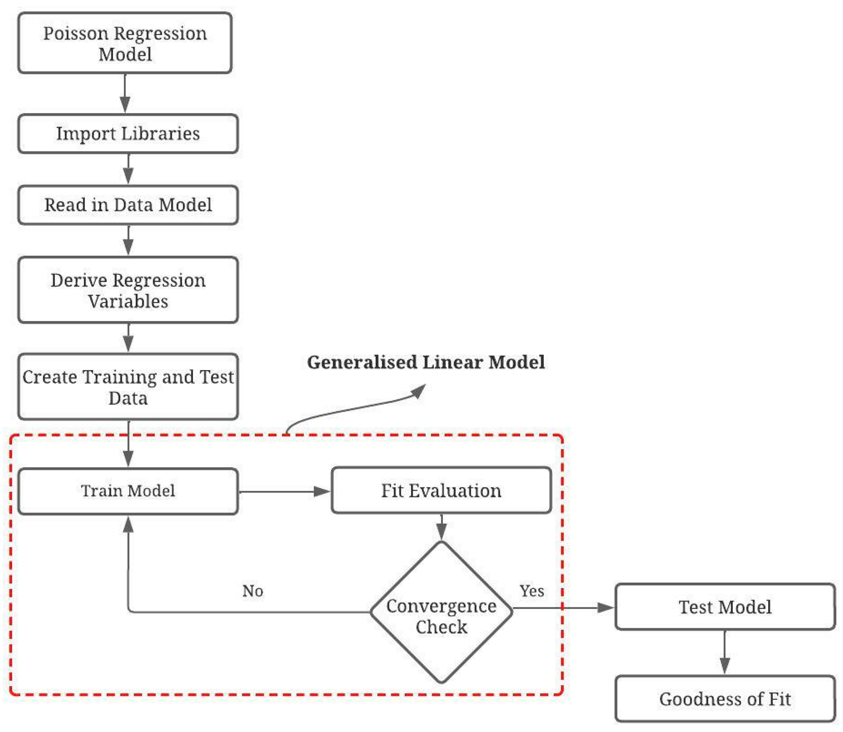
Training algorithms for prediction model continuous valued functions [33]. An algorithm that first imports the needed libraries such as Statmodel (necessary to train the model using GLM) to do this. The Pandas library was then used to read the data and derive the regression variables to be considered. A random data set that consists of 80% of the data is then created. The remaining 20% of the data will then be used for testing. Using the Statmodel GLM, the model is then trained on the training data set. The model is then tested on the remaining 20% of the data and the results are evaluated using the ‘goodness-of-fit’ measure. The designed algorithm is provided below (Figure 1).

Figure 1. Training algorithm.

3. Exploratory Data Analysis

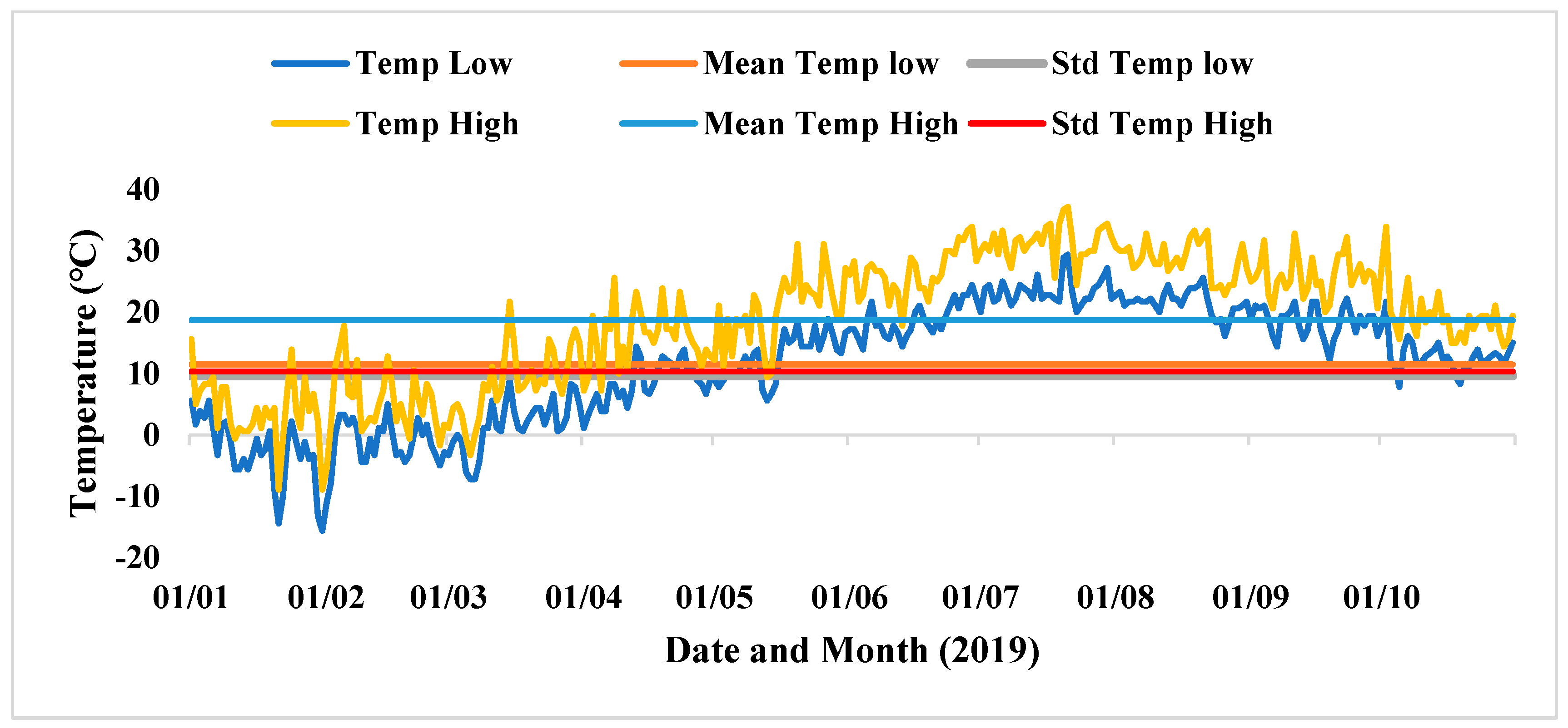
The graph below shows the average of two high and two low temperatures read from the data. To determine the variation from the average, the mean and standard deviation were also determined and plotted as seen in Figure 2.

Figure 2. High and low temperature vs. time series with mean and standard deviation.

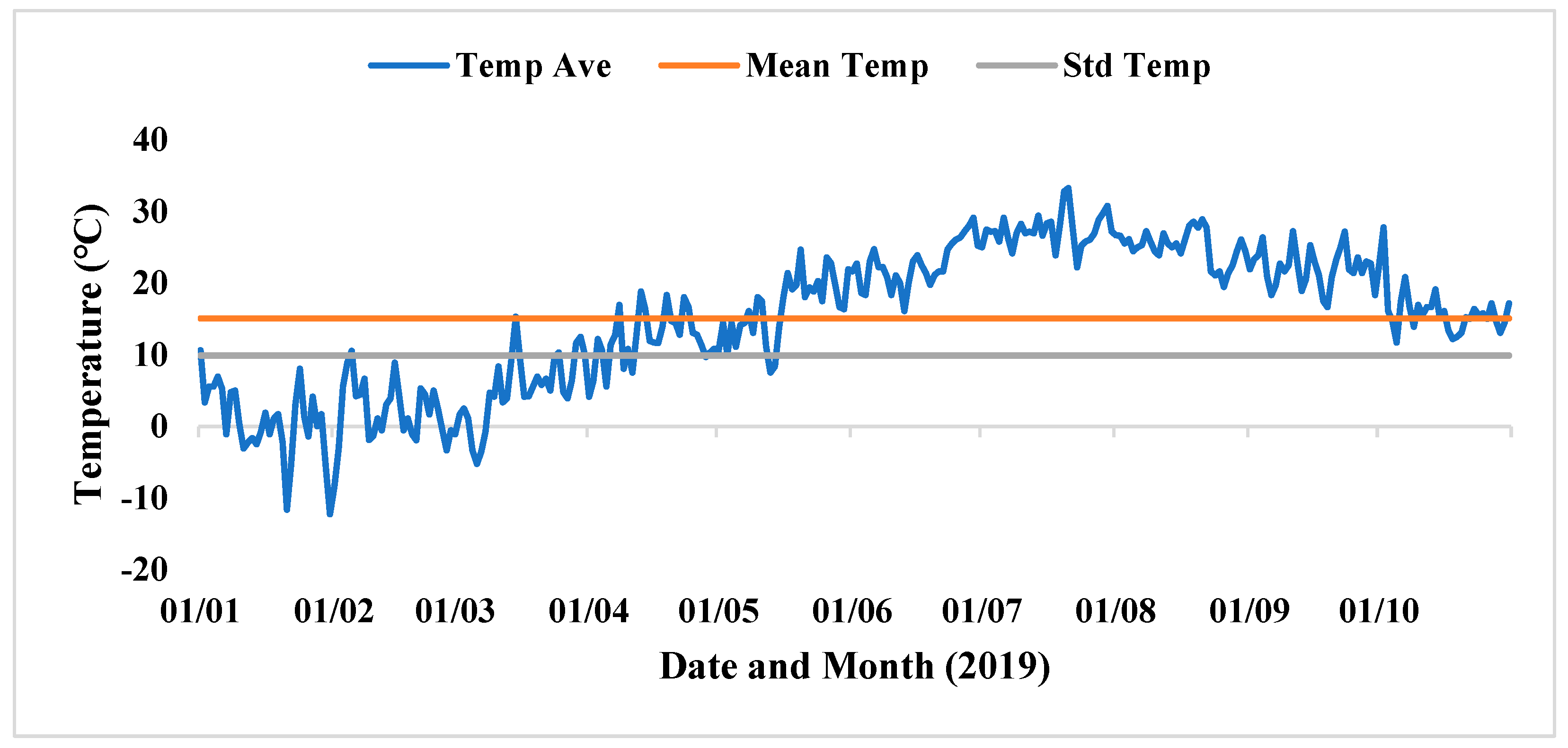
The average temperature vs. time series was also studied. The following Figure 3 was obtained.

Figure 3. Average temperature vs. time series with mean and standard deviation.

Sensitivity analysis was performed on the average temperature to understand the variation in the data used. The period of interest was one year. The results of this analysis are shown in Figure 4.

Figure 4. Average temperature vs. time series (sensitivity analysis).

It is clear from the blue line in Figure 4 that variations in the average temperature does have an impact on the model predictions (outputs), i.e., an increase in trip counts is observed with an increase in temperature and vice versa. Further details on the sensitivity analysis performed will be provided in Section 4.2 of this paper.

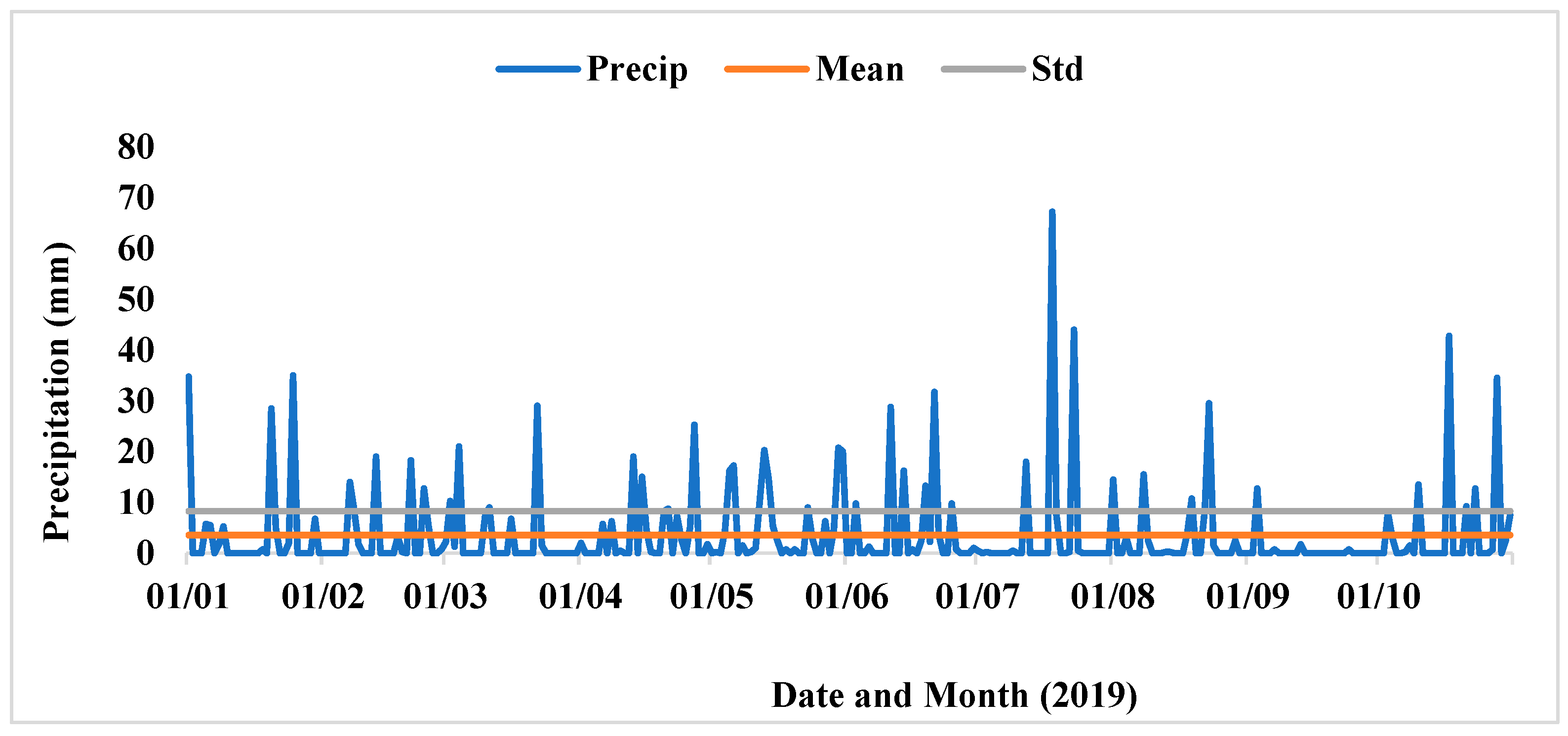
With reference to precipitation, no real variation or patterns in the data were observed when considering the precipitation parameter as seen in Figure 5 with the data currently used. So, it can be concluded that precipitation will be negligible in the output of this model. However, the model has taken into consideration the precipitation factor, and it should be noted that for regions in the world that have significant precipitations at different times of the year, precipitation would then become significant. The model would then predict trip counts under these conditions. Hence, this model aims not only to be used in an isolated region, but anywhere in the world, even in regions that have extreme temperature and precipitation changes.

Figure 5. Precipitation vs. time series with a mean and standard deviation.

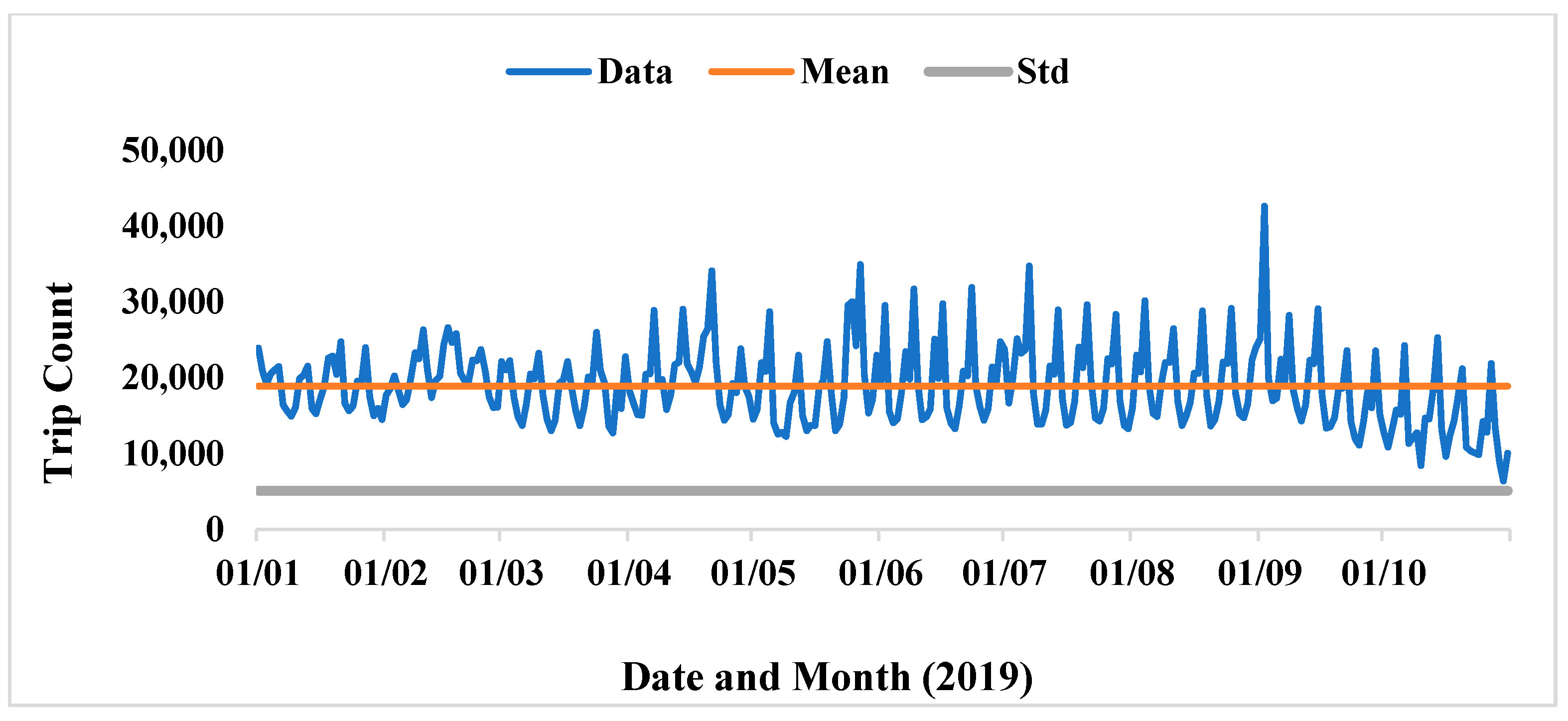
As done with temperature and precipitation, a plot for the counts with mean and standard deviation calculated was obtained as shown in Figure 6.

Figure 6. Trip count vs. time series with mean and standard deviation calculated.

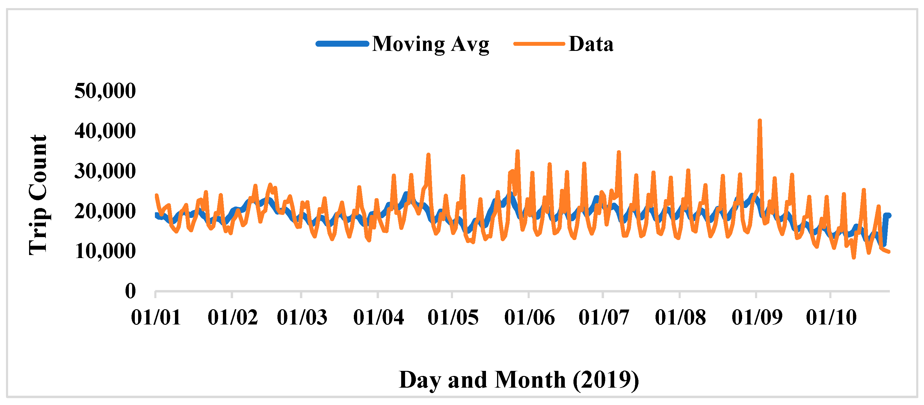
The moving average for the same trip count shown in Figure 6 was taken with a sample window of 10 days. This is used to forecast further data as depicted in Figure 7. This window size chosen as appropriate for this study was established through trial-and-error tuning/testing. The details at various sizes were observed, i.e., at a sample window size of 1, 5, 10, 20, 50 and 100. It was observed that at a window size higher than 10, irrelevant information started being captured. At the same time, anything below a value of 10 did not capture sufficient details. At a value of 10, the sliding window size provided the necessary detail needed for this model.

Figure 7. Moving average of trip count vs. time series.

4. Results and Discussion

In this section, the prediction model is verified. Once the regression model has been verified, it can be used to predict trip counts on any given day in a year, and in any weather condition possibly allowing better quantification of total fuel demand throughout interest. This would assist in calculating the demand that hydrogen refuelling stations must cater to. Since no actual data are available on the refuelling behaviour of HFVs in South Africa, this prediction model can provide useful insights and trends for refuelling of HFVs in the country, once adoption kicks off.

4.1. Verification of Model Performance

Validating the performance of the model was done by matching the outputs to real data points and observing how much the outputs of the model ‘deviated’ from actual data points (trip counts) as well as assumptions made. The results of the model training are detailed below.

From the results, it is evident that all the regression coefficients, $\beta$, are statistically significant at the 95% confidence level since their p-value is less than 0.05 except for precipitation which can be overlooked. It should be noted that the data were limited to 254 days, i.e., does not include a full year.

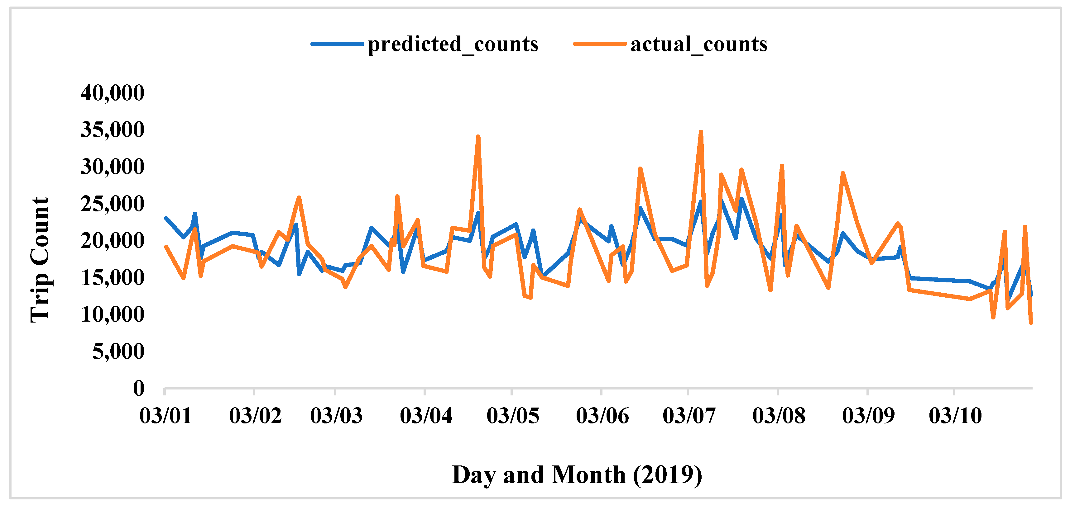
If the predictions are tested the following is obtained:

From this, it can be concluded that the model seems to be tracking the trend accurately with only a few outliers identified as seen in Figure 8. Moreover, it should be noted that precipitation was not taken to be an influential factor although this contradicts studies such as [34] that note that precipitation does indeed influence trip counts and fuel economy of a vehicle.

Figure 8. Predicted counts vs. actual counts.

When comparing the actual data with the predicted data, the following is obtained as seen in Figure 9 (a regression line was added showing the trend in the data).

Figure 9. Actual vs. predicted trip count trend.

One of the requirements for the Poisson regression model is that the mean and variance should be equal. This is a common failure for this type of model [30]. Hence the model was further tested to determine its accuracy using this assumption, i.e., variance is equal to the mean.

From Table 4 the ‘goodness-of-fit’ is indicated. It is noted that the deviance and the Pearson chi-square are too large, i.e., using a simple Poisson regression model does not provide an optimal fit. Moreover, it is evident that the degrees of freedom (DF) residuals are 234, and p = 0.05. Comparing to the chi-squared value that should be obtained (270.684), which is var less than 2.09 × 10⁵. Hence it can be concluded that this model alone does not have a good fit. In most cases the variance is either greater than or less than the mean in real-world data sets, this is known as over-dispersion or under-dispersion, respectively. The mean recorded when using the Poisson regression model instead of the generalised Poisson regression model was 18,895.92; the variance was found to be 26,034,786.04. Since the variance is larger than the mean, the data were over-dispersed, and the primary assumption of the Poisson model does not hold. This falls in line with studies such as [30] that indicate that a generalised Poisson regression model (GP-1) is required as it does not rely on the ‘variance = mean’ assumption. When using the generalised Poisson regression model (GP-1) instead of the Poisson regression model, the following results are obtained as seen in Table 5.

Table 4. Generalised Poisson Regression Results.

Generalised Poisson Regression Results
Dependent Variable:	COUNT		No. of Observations		254
Model:	GeneralisedPoisson		Df Residuals:		247
Method:	MLE		Df Model:		6
			Pseudo R-square:		0.02773
			Log-likelihood:		−2444.2
Converged:	TRUE		LL-Null:		−2513.9
Covariance Type:	Nonrobust		LLR p-value		1.33 × 10−27
	Coeff	Std error	z	p > |z|	[0.025	0.975]
Intercept	9.7958	0.051	192.114	0	9.696	9.896
Day	−0.0032	0.001	−2.319	0.02	−0.006	−0.001
Day of the week	0.0737	0.007	10.973	0	0.061	0.087
Month	−0.047	0.007	−7.126	0	−0.06	−0.034
High temperature (°C)	−0.0009	0.005	−0.185	0.853	−0.01	0.008
Low temperature (°C)	0.0123	0.005	2.35	0.019	0.002	0.023
Precipitation (mm)	−8.85 × 10−5	0.002	−0.059	0.953	−0.003	0.003
Alpha	26.5632	1.296	20.933	0	24.076	29.05

Table 5. Generalised Poisson Regression Results using GP-1.

Generalised Poisson Regression Results
Dependent Variable:	COUNT		No. of Observations		254
Model:	GeneralisedPoisson		Df Residuals:		247
Method:	MLE		Df Model:		6
			Pseudo R-square:		0.02773
			Log-likelihood:		−2444.2
Converged:	TRUE		LL-Null:		−2513.9
Covariance Type:	Nonrobust		LLR p-value		1.33 × 10−27
	Coeff	Std error	z	p > |z|	[0.025	0.975]
Intercept	9.7958	0.051	192.114	0	9.696	9.896
Day	−0.0032	0.001	−2.319	0.02	−0.006	−0.001
Day of the week	0.0737	0.007	10.973	0	0.061	0.087
Month	−0.047	0.007	−7.126	0	−0.06	−0.034
High temperature (°C)	−0.0009	0.005	−0.185	0.853	−0.01	0.008
Low temperature (°C)	0.0123	0.005	2.35	0.019	0.002	0.023
Precipitation (mm)	−8.85 × 10−5	0.002	−0.059	0.953	−0.003	0.003
Alpha	26.5632	1.296	20.933	0	24.076	29.05

From these results, it is evident that the model training was able to converge as shown by the True field by ‘converged’; if this was false the model would have failed and would need modifications. Moreover, it is noted that all the variable coefficients are statistically significant at the 95% confidence level except for precipitation and high temperature. Moreover, note the MLE (Maximum Likelihood Estimate) = −2350.3 is greater than the null-models MLE of −2422.0. Additionally, the Likelihood Ratio (LR) test’s p-value is extremely small = 1.797 × 10⁻²⁸ which shows this does better than just a simple intercept only method.

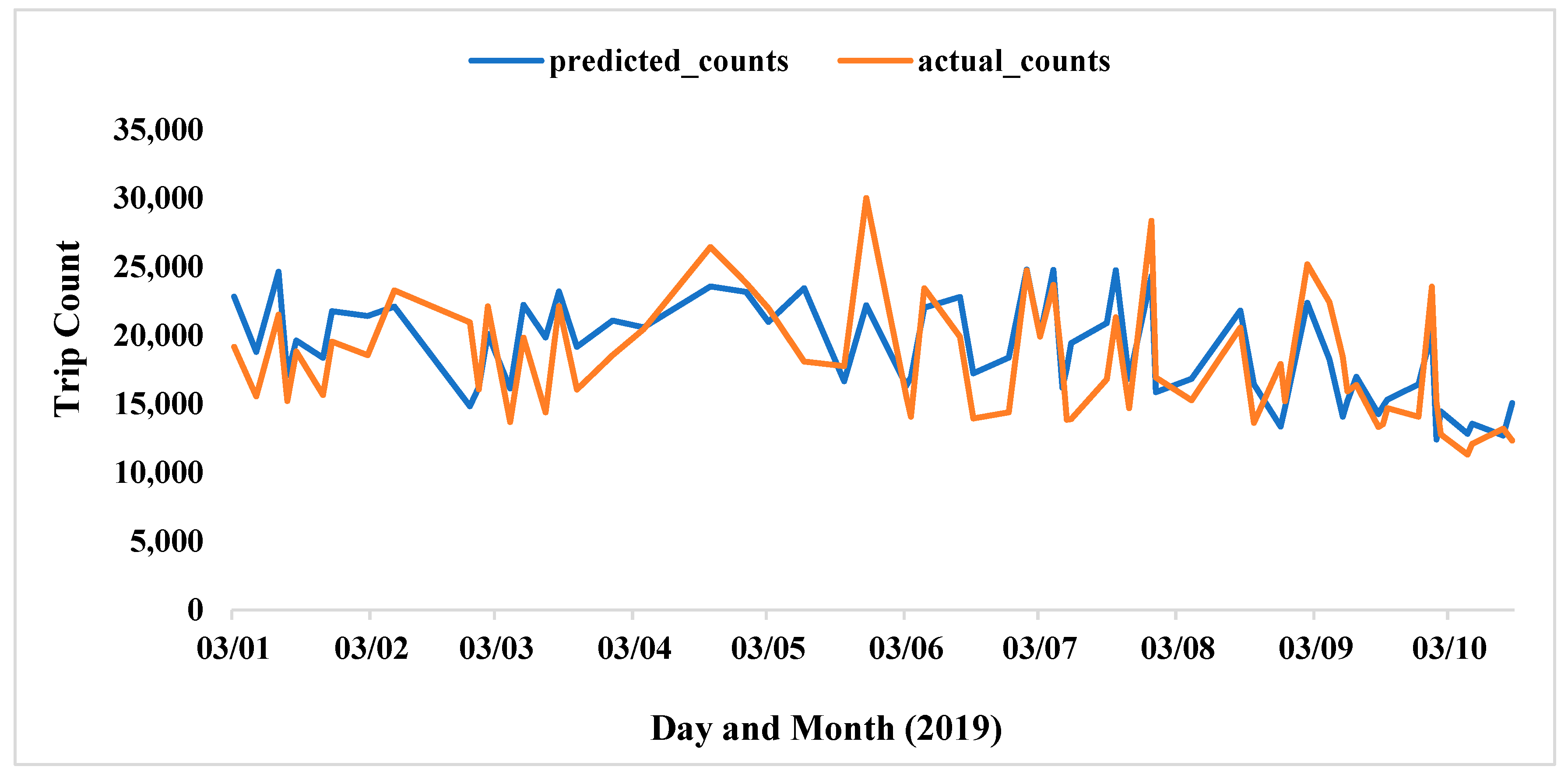
Furthermore, the MLE for the Poisson model was −95,989 compared to the GP-1 of −2350 which shows that the GP-1 model has a better goodness-of-fit. Moreover, Figure 10 below shows that the GP-1 model predicts quite closely compared to the actual data:

Figure 10. Predicted vs. actual car trip counts using GLM.

4.2. Sensitivity Analysis Based on Training Sets

By performing sensitivity analysis, it is possible to assess and quantify how the uncertainty of the outputs obtained from the model is related to the uncertainty of the inputs, that is, the sensitivity of the model to changes in the parameters and data on which it is built [35]. The sensitivity analysis is done to establish:

• Any errors in the model itself.
• Calibration of model parameters.
• Relationship between model inputs and outputs.

Since a generalised Poisson regression model has been used in this study, it was important to validate the performance of the model under modified conditions. The sensitivity analysis was performed to verify the influence of assumptions on the accuracy of the model to identify the key value drivers that impact the outcomes of the model, as well as to provide a clearer understanding of the trends and the assumptions made. The model is designed to predict trip counts on any given day of the year and in any weather condition. Parameters, used in the regression model, and of interest, include temperatures (high and low), precipitation and trip counts. It should be recalled that the algorithm for the regression model will try to fit the observed counts y to the regression matrix X [30].

The table below shows the different correlation values based on using various training percentages. This means that a certain percentage of the data were used to train the model. It is noted that training sets that use less than 50% have a poorer correlation compared to those above 50%. The best correlations were found at 0.7, i.e., 70% of the data were used to train the model.

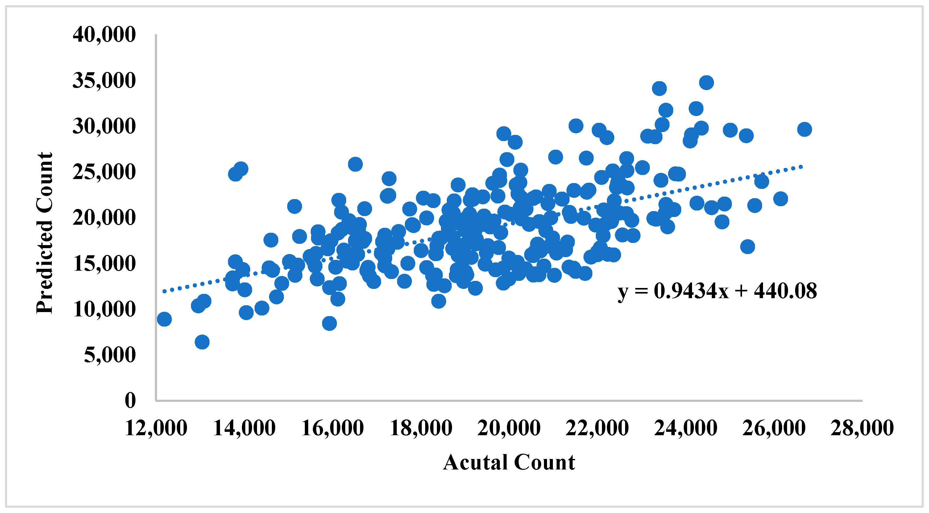
At a training percentage of 0.1, as seen in Figure 11, the correlation achieved between the actual data and the predicted data generated by the model is equal to 0.53. As the training percentage is increased to 0.5, the correlation between the actual and predicted data increases to 0.68 as seen in Figure 12.

Figure 11. Training % at 0.1 data.

Figure 12. Training % at 0.5 data.

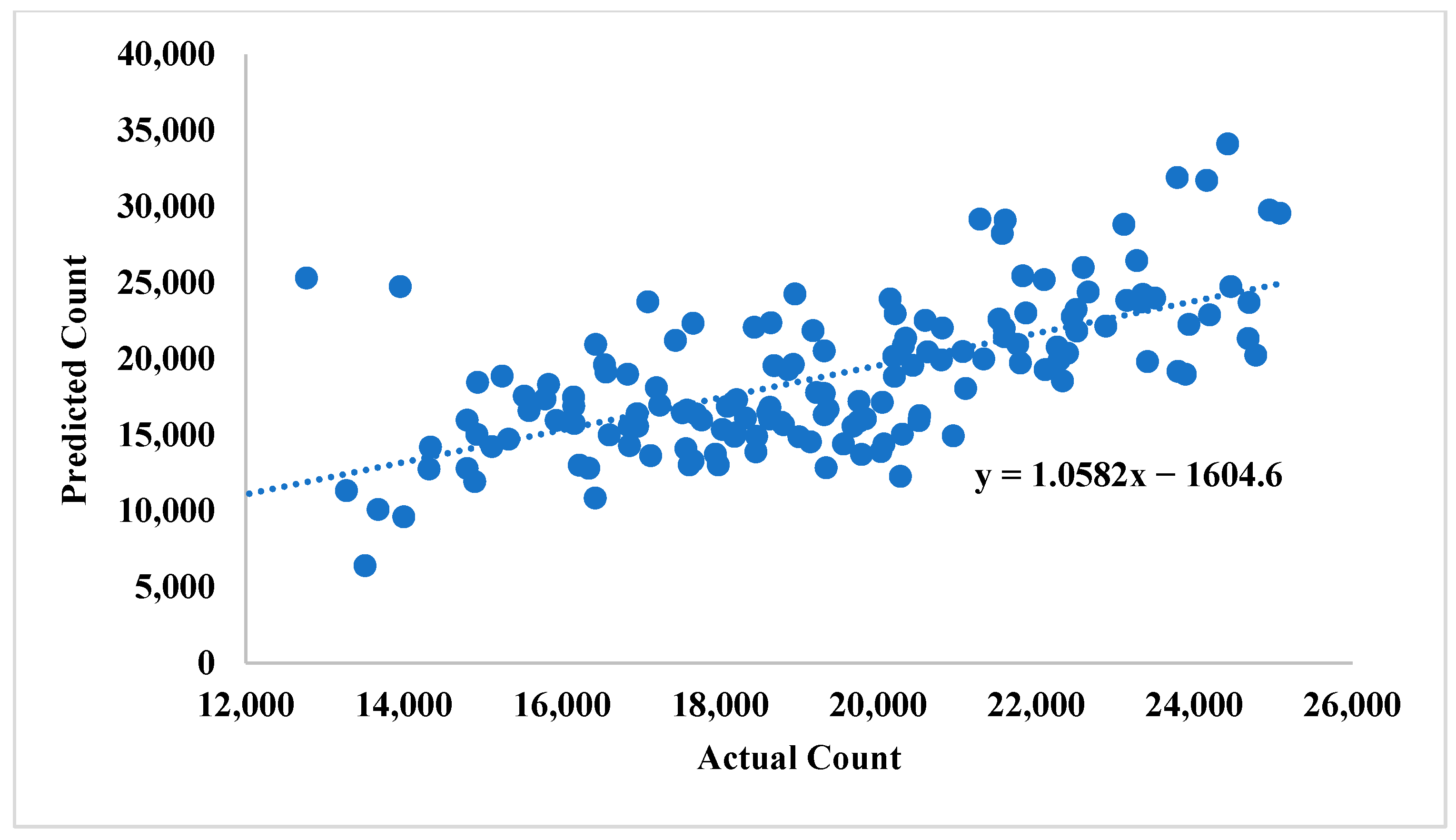
To further test the trend, the correlation at a training percentage of 0.7 was also noted. Once again, it is evident that the correlation between the actual and predicted data increases as the training percentage increases. At 0.7, the correlation between the actual data and predicted data was 0.72. This was the highest correlation value achieved, indicating that the training percentage of 0.7 was optimal for the model. This is shown in Figure 13.

Figure 13. Training % at 0.7 data.

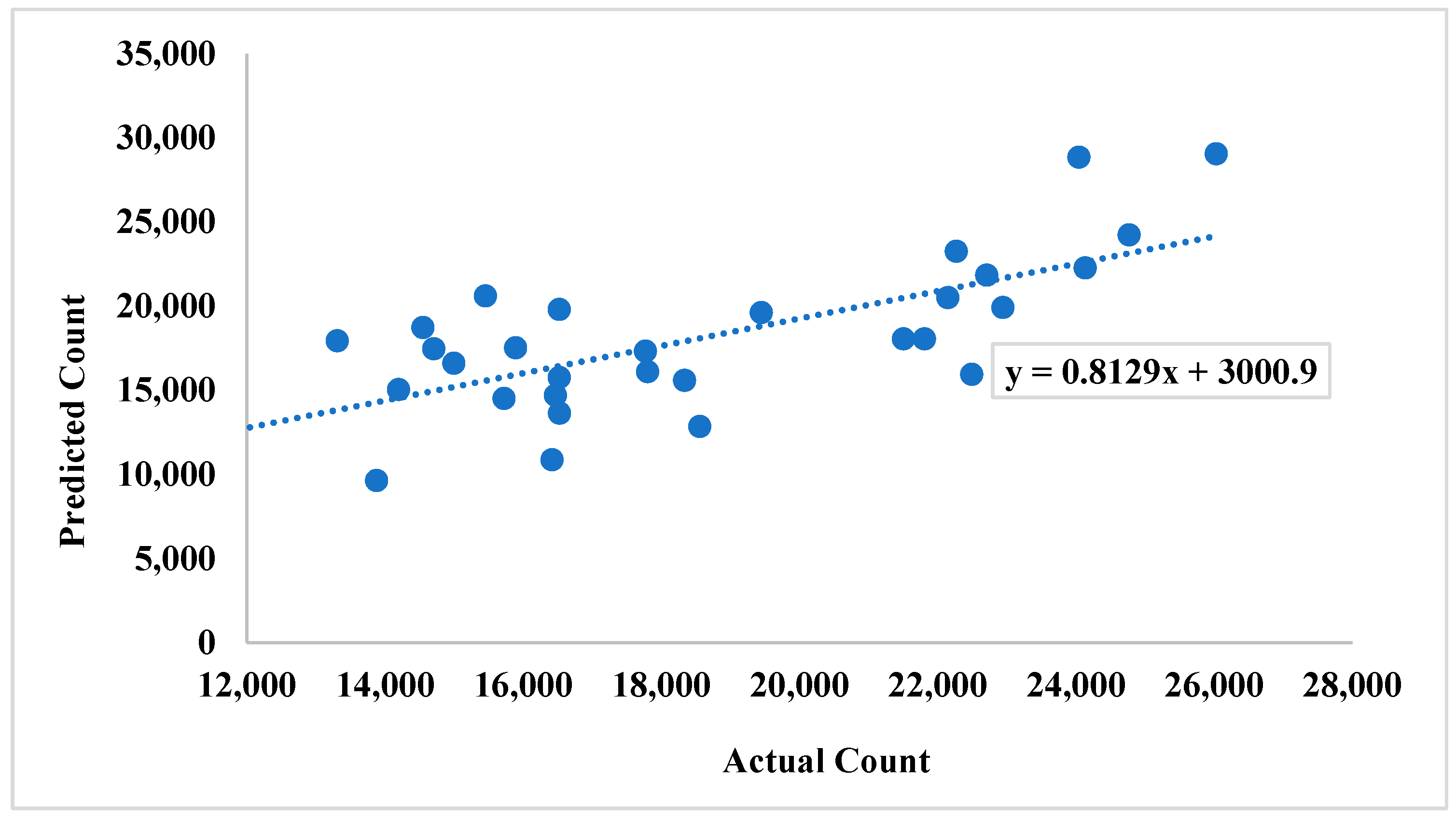
Any increase in training percentage higher than 0.7 resulted in a lower correlation factor as seen in Figure 14. At 0.9 a correlation factor of 0.68 is achieved. This result is due to the fact that a small data set using less training data was used, hence the parameter estimates exhibit greater variance. With fewer testing data, the performance statistics would have greater variance.

Figure 14. Training % at 0.9 data.

5. Conclusions

Studying and predicting the refuelling patterns and behaviours of vehicle users can provide valuable information about the infrastructure requirements and predicted refuelling patterns. The established model can also be used within the South African upon further uptake of HFVs in the country, and once HFV trip data are available.

The prediction model developed in this study takes into consideration the fact that real-world datasets are either under- or over-dispersed to predict future trip counts, and consequently advise the predicted fuel consumption.

This algorithm provides a useful opportunity to explore further HFV research by analysing the outputs of the algorithm, which currently is built on general vehicle data. Furthermore, this algorithm can be used to draw analogies between general vehicles and HFVs, as well as analogies between cities of the same size across in South Africa, or even globally as the model can be used to predict driving trip counts. In terms of further research, the predictions provided by the model can prompt the question of how many refuelling stations is needed to cater for the number of refuelling trips predicted. Additionally, only 20% of the data were used for testing. Overall, this model allows the prediction of refuelling trip trends and inform refuelling infrastructure requirements for HFVs, once adoption increases and HFV data are available.