Imaging Domain Seismic Denoising Based on Conditional Generative Adversarial Networks (CGANs)

Abstract

A high-resolution seismic image is the key factor for helping geophysicists and geologists to recognize the geological structures below the subsurface. More and more complex geology has challenged traditional techniques and resulted in a need for more powerful denoising methodologies. The deep learning technique has shown its effectiveness in many different types of tasks. In this work, we used a conditional generative adversarial network (CGAN), which is a special type of deep neural network, to conduct the seismic image denoising process. We considered the denoising task as an image-to-image translation problem, which transfers a raw seismic image with multiple types of noise into a reflectivity-like image without noise. We used several seismic models with complex geology to train the CGAN. In this experiment, the CGAN’s performance was promising. The trained CGAN could maintain the structure of the image undistorted while suppressing multiple types of noise.

1. Introduction

A seismic image is a profile that indicates the acoustic impedance discontinuities below the subsurface. With an accurate seismic imaging profile, geophysicists and geologists can identify complex geology (fault, salt, folding, etc.) and locate resources in the deep earth interior. To acquire a high-resolution imaging profile, we need high-density spatial sampling and pure primary reflection seismic data. However, this is difficult to realize in practice. First, it is hard to achieve high-density spatial sampling in real field seismic data acquisition, especially in land surveys. Mountains, rivers, and other complex terrain will affect the installation of geophones and seismic sources. Second, in most cases, the seismic imaging is based on the kinematics of the primary reflection wavefield, and there may be multiple types of noise (e.g., train and tidal noise, other unwanted waveforms) contaminating the primary reflection data. As a result, the migrated imaging profile has different types of noise, which should be eliminated to enhance the signal-to-noise ratio (S/N) [1,2]. Noise can be classified as coherent or incoherent. Noise suppression is an essential step in reflection seismic data processing [3]. Therefore, the main challenge is to remove the noise while preserving the seismic signals [4]. Several methods have been developed to attenuate random noise, e.g., the t-x and f-x prediction methods [5,6], median filtering (MF) methods [7,8,9], sparse transform-based methods [1,10,11,12], singular spectrum analysis (f-x SSA), and other effective and improved versions of the above [13,14].

Recently, deep neural networks (DNNs) [15] have attracted considerable attention as a promising framework that provides state-of-the-art performance for image classification, speech recognition, target detection, and many other fields related to the processing of unstructured data. The network consists of multiple layers for learning the representation of a given datum. Among network architectures, the convolutional neural network (CNN) is the most popular deep neural network architecture for image classification [16], segmentation [17], and restoration [18]. The convolutional neural network uses convolution, pooling, and weight sharing to replace the multilayer perceptron (MLP) on several layers of the deep neural network, which greatly reduces the parameters that need to be trained. A convolutional neural network only made of convolutional layers is referred to as a fully convolutional network (FCN) [19], and this has proved to be a pixel-to-pixel, end-to-end solution for semantic segmentation. In the field of seismology, convolutional neural networks have been successfully applied in first-break picking [20], fault detection [21,22], full-waveform inversion [23], salt body classification [24], seismic facies classification [25], noise attenuation [26,27], impedance inversion [28], velocity model building [29], seismic phase classification [30], and Q model estimation [31].

Among the many types of network architecture, the generative adversarial network (GAN) [32] is essentially a generative model that learns a collection of data and generates artificial objects that are similar to those found in real life. It is a novel method, and the idea behind the generative adversarial network is straightforward. This type of network consists of two types of deep neural networks: a generator (G) and a discriminator (D). G creates fake objects, and D can distinguish generated objects from real ones. G and D are like two players competing against each other; a balance is reached when both of them play optimally, assuming that their opponent is optimal. The generative adversarial network has been a research hotspot in recent years, and several networks with different structures have been proposed [33,34,35] for generating a specified area of data. The conditional GAN is an extension of the conventional generative adversarial network [36]. The only difference between conditional and conventional GANs is that the former additionally provides a given datum as the input of the generator rather than random noise only. Conditional GANs can be used to realize super resolution [37], image deblurring [38], and image-to-image translation [39].

In this paper, we refer to the deblurring GAN and the pix2pix GAN, which belong to the branch of conditional GANs, and their potential to realize seismic imaging domain denoising. First, we introduce the data preparation, including the imaging data acquisition and the data augmentation. Then, we introduce the architecture of the conditional GAN and the objective function. After that, the evaluation method and examples are illustrated to validate the feasibility of our method. Finally, we offer some concluding remarks.

2. Theory and Methodology

The proposed conditional GAN solves an image-to-image translation problem, i.e., how to transfer a migration image with multiple types of noise into an image corresponding to a reflectivity model without noise. This theoretical section consists of three parts. In the first part, we introduce the architecture of the proposed conditional GAN, including the generator and the discriminator. Then, in the second part, the data preparation and data augmentation procedures are described. In the last part, the object function and the training details are discussed.

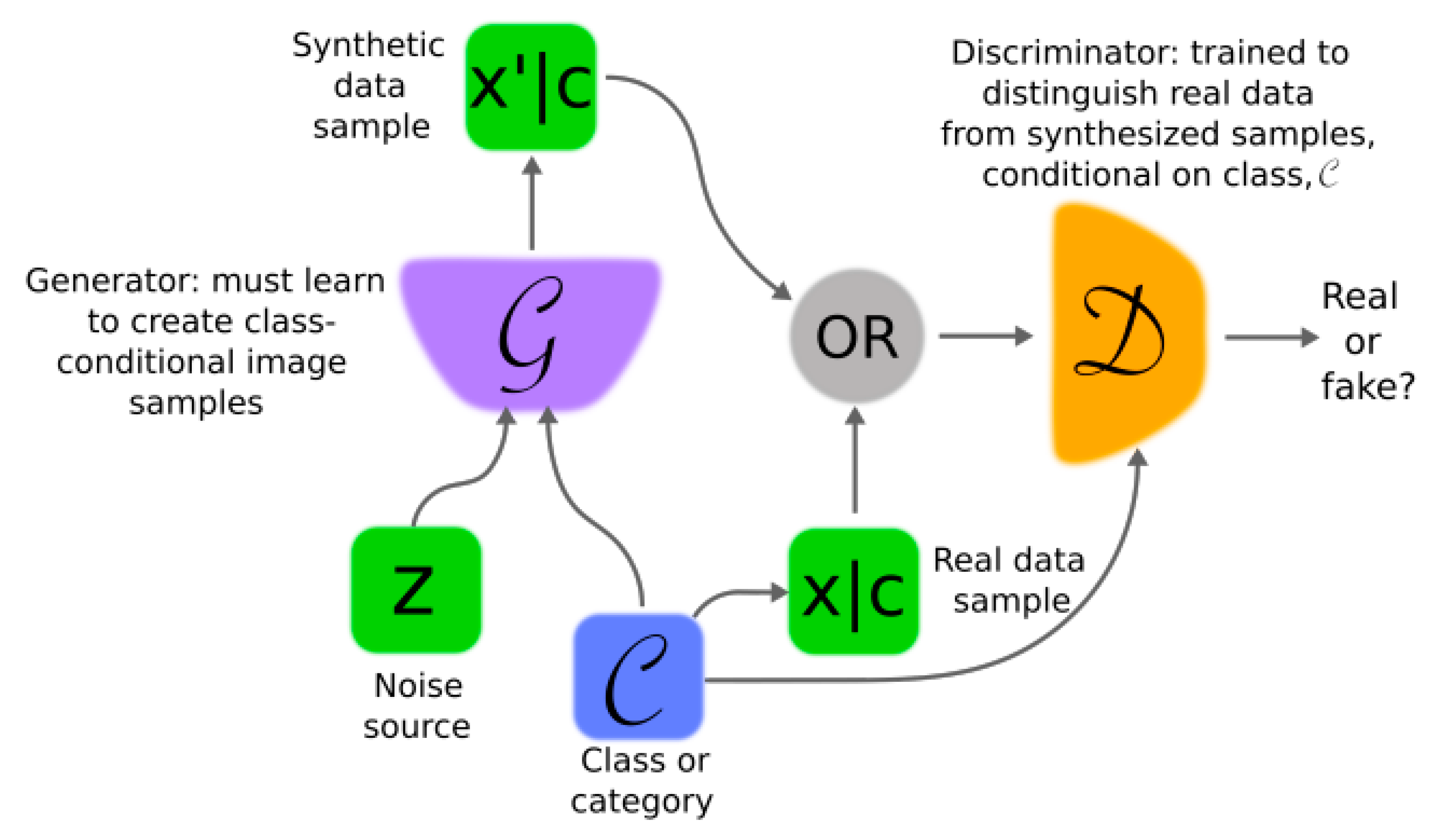
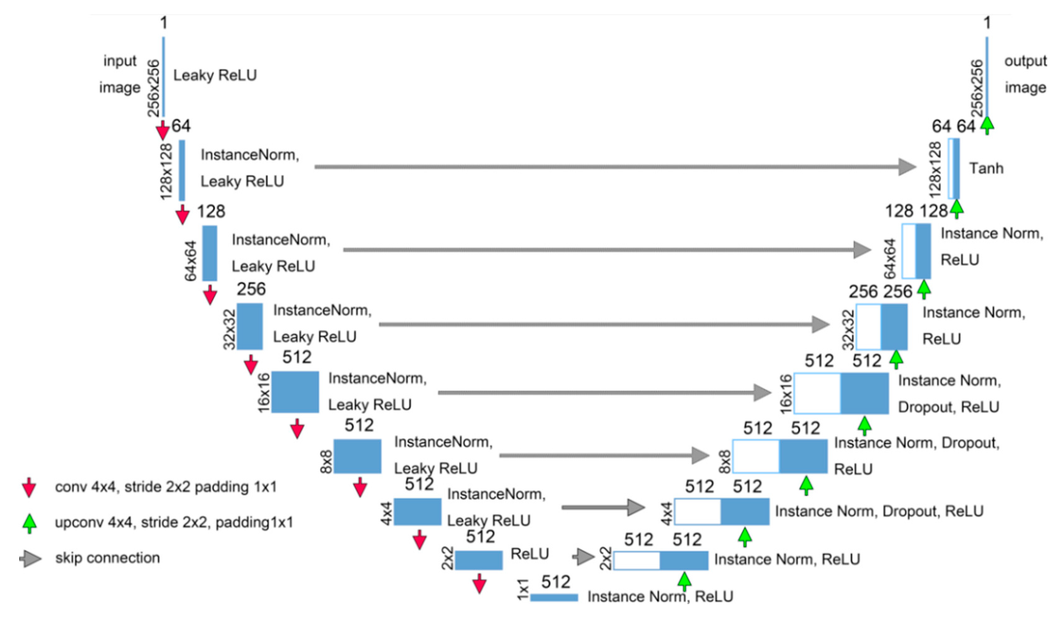
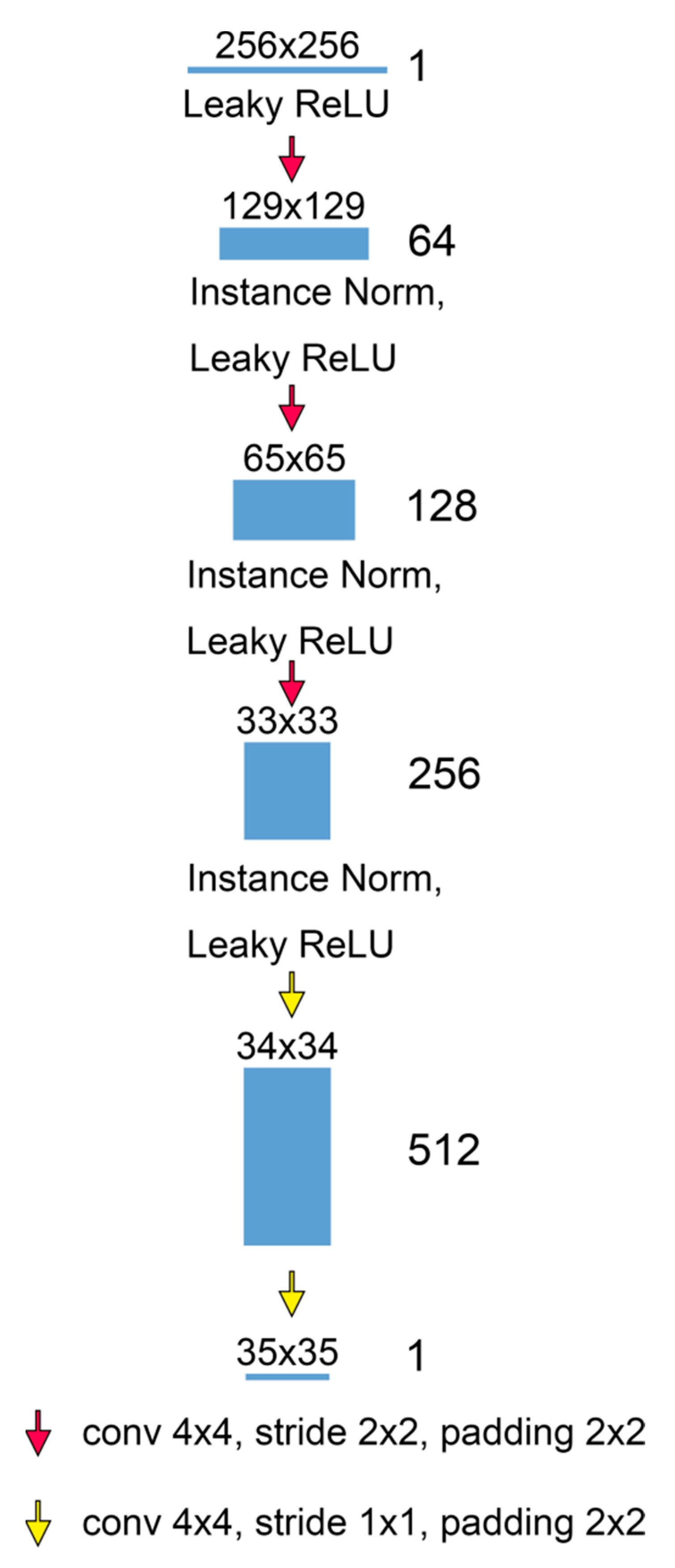
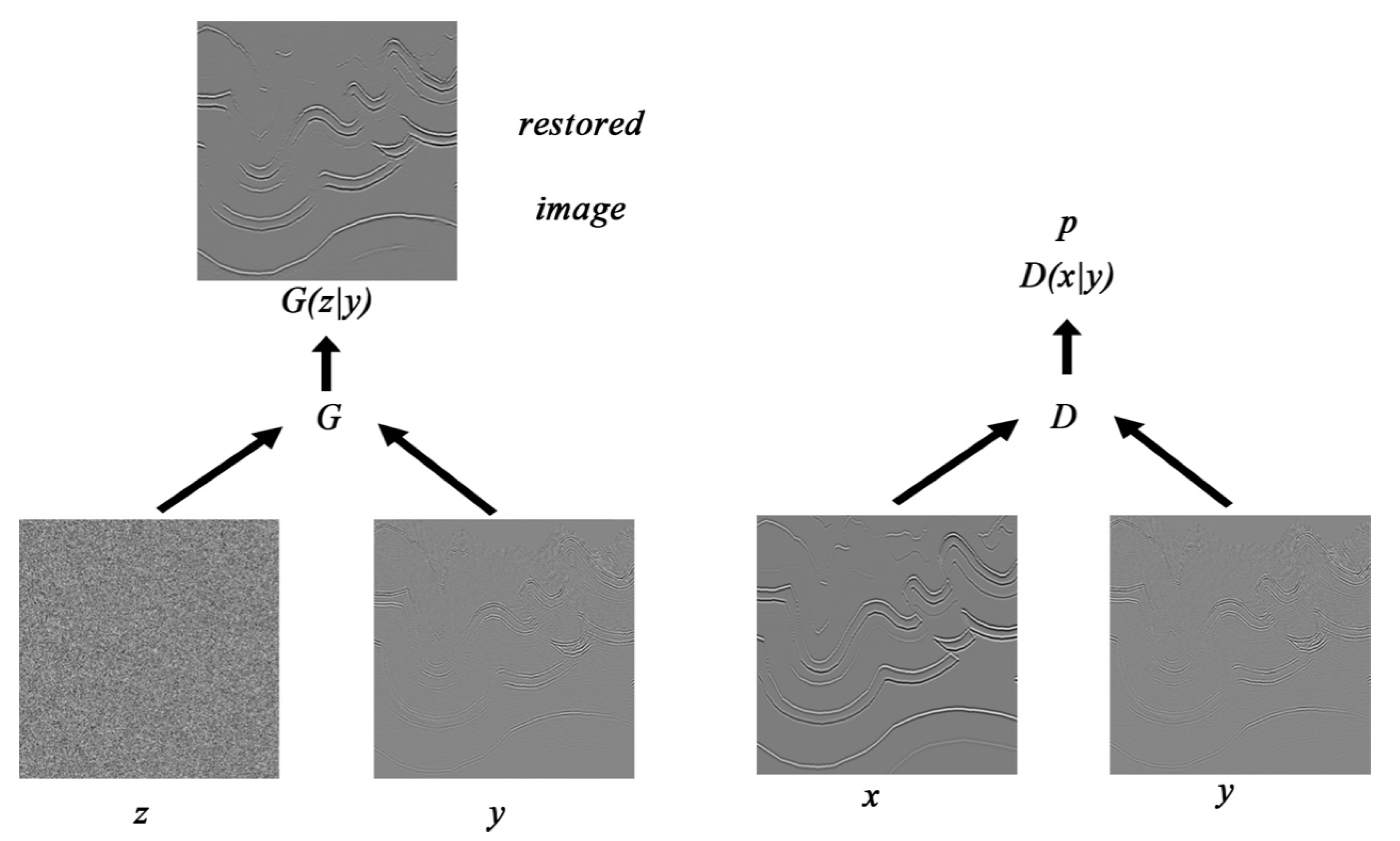
3. The Architecture of the Conditional GAN for Seismic Imaging Denoising

For our purposes, it is necessary for the reflection events to be undistorted and the noise removed. We trained the GAN on the basis of a deblur GAN [38], which was developed from a pix2pix network and realized an end-to-end method for motion deblurring [39]. The advantage of a deblurring GAN is that it maintains the structural similarity of the image while improving the visual performance, which accords with the target of our research. The source code of the deblur GAN is available at https://github.com/KupynOrest/DeblurGAN.

The deblurring GAN is part of the branch of conditional generative adversarial networks [36], which in turn are extensions of the general GAN [32]. The generative adversarial network consists of a generator (G) and a discriminator (D), and these can be chosen arbitrarily. A typical architecture of a conditional GAN is shown in Figure 1. In our network structure, we follow the configuration of the pix2pix GAN that uses U-net as the generator and the Markovian discriminator (patch GAN) as the discriminator.

U-net is named for its U-shaped network architecture, and it was originally designed for biomedical segmentation (see Figure 2) [17]. The traditional convolutional networks used the sliding window technique, each pixel was classified individually (also known as convolution), which was quite time-consuming. U-net improves the working of convolutional neural networks significantly by combining a constrictive down-sampling path and a symmetrical expansive up-sampling path with skip connections. It requires small number of training examples, unlike the traditional convolutional networks that used thousands of annotated training samples. The contracting path follows the typical architecture of a convolutional network. In the down-sampling stage, the image size progressively decreases while the number of channels increases. In the down-sampling path, there are 8 convolution blocks, where each block has a convolution layer with 4 × 4 padding, followed by a ReLU (rectified linear unit) with a slope of 0.2, and a 2 × 2 max pooling operator with 2 strides. The rest of the layers adopt a leaky ReLU with a slope of 0.2 [40] and instance normalization.

When the dataflow passes through the bottleneck layer in the middle of the network, the process is then reversed. One advantage of a fully connected neural network model is that the input size of the image is unrestricted. Thus, we can input an image of arbitrary size without modifying the architecture. For an image translation task, it is necessary to maintain lots of low-level information. An efficient method is to shuttle the low-level information across the network. U-net adopts a skip connection between each layer $i$ and layer $n-i$, where $n$ is the depth of U-net. As a result, U-net has proved to be effective on a small dataset while avoiding overfitting [31].

The architecture of the adopted U-net is shown in Figure 2. The encoder–decoder architecture has 16 layers in total, with 54,409,603 parameters to be trained. The encoder part consists of 8 convolutional layers. Except for the first layer, where the batch norm is not applied, the rest of the layers adopt a leaky ReLU with a slope of 0.2 [40] and instance normalization [41]. In the decoder part, there are 8 transposed convolutional layers [42]. The first 7 layers adopt a ReLU [43] and instance normalization. For the last layer, tanh is applied as the nonlinear activation function. Dropout [44] with a 50 percent chance is applied in the middle layer of the decoder part to enhance the generalization performance and alleviate overfitting.

Typically, the discriminator is a relatively simple network. For the seismic denoising problem, the discriminator not only needs to ensure that the low-frequency structure is undistorted, but it also needs to distinguish high-frequency reflection events from multiple types of noise. The patch GAN [45], also a classical model, has been proposed as a texture loss model. It assumes that the independence between pixels is greater than a patch diameter and regards the image as a Markov random field. The patch GAN runs in a convolutional way across the image, each time penalizing a part of the image at the patch scale. The ultimate output of the discriminator is the average of all responses of the patches.

The architecture of the patch GAN discriminator is shown in Figure 3. The patch GAN discriminator is a 5-layer FCN model with 2,764,737 parameters. Except for the last layer, instance normalization and a leaky ReLU with a slope of 0.2 are applied. The ultimate score of the discriminator is the average of the discriminator output.

4. Data Preparation

A conditional GAN needs image pairs “AB” for its training samples. In our method, the migration image is the raw image “A”, which is to be denoised, and the reflectivity model is the desired image “B”.

Reverse time migration (RTM) is a robust and standard seismic imaging algorithm. It is based on a two-way wave equation, either the acoustic wave equation or the elastic wave equation, which reconstructs the wavefield towards the reflectivity model. In theory, RTM can handle complex geology, highly dipping reflectors without angle limitation, and strong velocity discontinuities. We used reverse time migration to generate image “A” of the image pair using both finite-difference-based acoustic RTM [46] and grid-method-based elastic RTM [47] techniques. This means that the image library for training included both acoustic and elastic images. The imaging profile can be regarded as the image of reflectivity when the density changes are not dramatic, which can be approximated by $\frac{v_1-v_2}{v_1+v_2}$, where $v$ is the interval velocity. We first generated the reflectivity image by using the accurate velocity model. Then, we convolved the reflectivity model with a Ricker wavelet with a dominant frequency of 25 Hz to generate image “B”.

The migration image is a relative value rather than the real reflectivity value, which makes the scale between the migration profile and the accurate reflectivity data different. We performed normalization and used the grayscale image to make sure that the image pairs were in the range of 0 through 255.

Data augmentation provides extra training data derived from raw data when the quantity of training samples is not adequate. With proper data augmentation, a deep neural network can better discover meaningful information and enhance its data prediction quality. In our method, we adopted random cropping, horizontal flipping, and color jittering for data augmentation. The crop size was 256 by 256, the brightness was chosen uniformly from 0.8 to 1.2, and the contrast was chosen uniformly from 0.8 to 1.2. Several image pairs are shown in Figure 4.

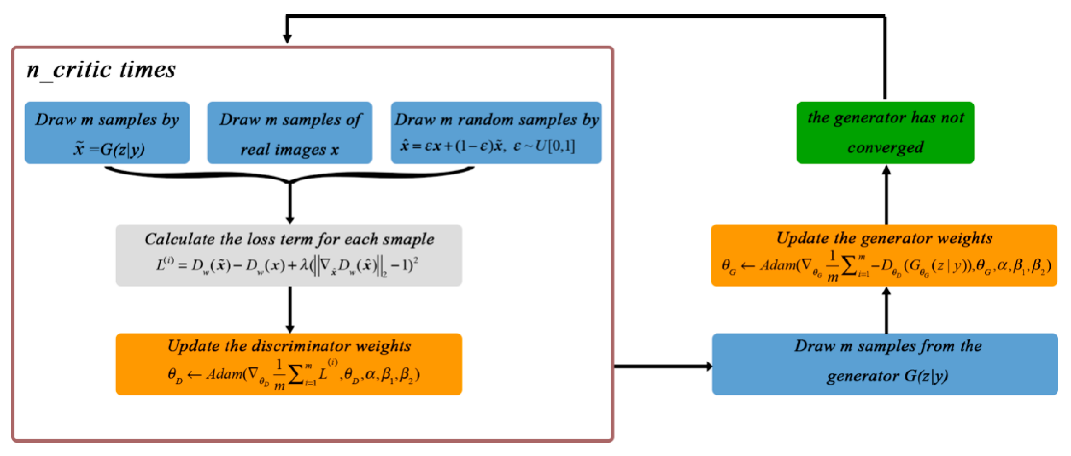
5. Objective Function

A generative adversarial network comprises two parts, the generator and the discriminator, which compete with each other. On the one hand, the generator captures a conditioned data distribution and builds a conditional mapping function from a prior noise distribution $p_z(z)$ on the condition of an extra input $y$ to the data space $G(z|y)$, trying to fool the discriminator. On the other hand, the discriminator D estimates the conditional probability $x|y$ that the sample came from the training data $x$ on the condition of $y$ rather than G to distinguish the real from the fake. Figure 5 illustrates the structure of a conditional GAN. The generator and discriminator have independent objective functions and are trained iteratively.

In this part, we first introduce the loss function of the discriminator. Then, the loss function of the generator is illustrated. Finally, we introduce the structure similarity index to evaluate the performance of the trained GAN.

6. Loss Function of the Discriminator

The Wasserstein GAN with a gradient penalty (WGAN-GP) [48] was adopted as the loss function for training the discriminator. The WGAN-GP has proved to be strong and robust across a variety of GAN architectures by using the earth mover’s (also called Wassertein-1) distance rather than the Jensen–Shannon distance, which is used in traditional GANs. Moreover, the Wassertein-1 distance correlates with the performance of the GAN, which enabled us to evaluate the performance of the GAN using the value function, whereas the Jensen–Shannon distance would not have allowed this. In addition, the WGAN-GP uses a gradient penalty rather than simple weight clipping [49] to enforce the Lipschitz constraint, making the training process more stable. The loss function of the WGAN-GP consists of two terms, the Wassertein-1 term and the gradient penalty term, which can be expressed as

$$\begin{array}{r}{L}_D({\theta }_G,{\theta }_D)=\underset{\tilde{x}~{\mathbb{P}}_g}{\mathbb{E}}[D(G(z|y;{\theta }_G))]-\underset{x~{\mathbb{P}}_r}{\mathbb{E}}[D(x|y;{\theta }_D)]\\ +\lambda \underset{\widehat{x}~{\mathbb{P}}_{\widehat{x}}}{\mathbb{E}}[{({‖{\nabla }_{\widehat{x}}D(\widehat{x}|y;{\theta }_D)‖}_2-1)}^2]\end{array}$$

(1)

where $L_D$ is the loss function of the WGAN-GP, ${\theta }_G,{\theta }_D$ are the weights of the generator and the discriminator, respectively, $\mathbb{E}$ is the expectation, $x~{\mathbb{P}}_r$ is the real data, $\tilde{x}=G(z|y;{\theta }_G)~{\mathbb{P}}_g$ represents the generated samples, $\widehat{x}=\epsilon x+(1-\epsilon )\tilde{x}~{\mathbb{P}}_{\widehat{x}}$ represents the so-called random samples of the WGAN-GP, $\epsilon ~U[0,1]$ is a uniform random number between 0 and 1, $z~\mathbb{P}(z)$ is the latent variable, $y$ is the conditional information, and ${\mathbb{P}}_g,{\mathbb{P}}_r,{\mathbb{P}}_{\widehat{x}}$ are the model distribution, data distribution, and sampling distribution, respectively. The first two terms of Equation 1 are the original critic loss, and the second term is the gradient penalty term with the penalty coefficient $\lambda$. In our experiment, $\lambda =10$, as suggested for the WGAN-GP.

7. Loss Function of the Generator

The loss function of the generator also consists of two parts, the discriminator score part and an L1-norm context loss, which can be expressed as

$$\begin{array}{ll}{L}_G({\theta }_G)& =L_{GAN}+L_1\\ & =E_{y,z}-D(G(z|y;{\theta }_G);{\theta }_D)+{\mathbb{E}}_{x,y,z}{‖x-G(z|y;{\theta }_G)‖}_1\end{array}$$

(2)

where the first term $L_{GAN}$ is the discriminator score part, and the second term $L_1$ is the L1-norm context loss.

The L1-norm penalizes the distance between ground-true outputs, which also encourages the output relative to the input. The L2-norm may lead to a blurred output. As a result, the L1-norm provides better performance than the L2-norm in seismic image denoising. It has been proved by several GANs [38,39](Isola et al., 2017; Kupyn et al., 2017) that L1 + GAN is effective at creating realistic renderings that respect the input label maps.

The generator should minimize the generator loss while the discriminator tries to increase the discriminator loss. The final objective is

$$G^{*}=\arg \underset{{\theta }_G}{\min }\underset{{\theta }_D}{\max }{L}_D({\theta }_G,{\theta }_D)+\mu L_G({\theta }_G)$$

(3)

where $\mu$ is a hyperparameter for balancing the discriminator D and the generator G. In our experiment, we set $\mu =100$, as suggested for deblur GANs.

The training process of the GAN is illustrated in Figure 6. First, train the discriminator for $n_{critic}$ times and update the parameters of the discriminator. In our experiment, $n_{critic}=5$. Second, train the generator and update the generator parameters depending on the updated discriminator parameters. The two steps iterate until the generator converges to a stable state. Both the discriminator and the generator adopt the Adam optimization method (Kingma and Ba, 2014 [50]). There are three hyperparameters, $\alpha ,{\beta }_1,{\beta }_2$, introduced by Adam optimization, where $\alpha$ is the learning rate and ${\beta }_1,{\beta }_2$ are the coefficients for computing running averages of the gradient and its square. In our training process, the assignment of the hyperparameters was as follows: $\alpha =0.0001,{\beta }_1=0,{\beta }_2=0.9$.

8. Performance Evaluation

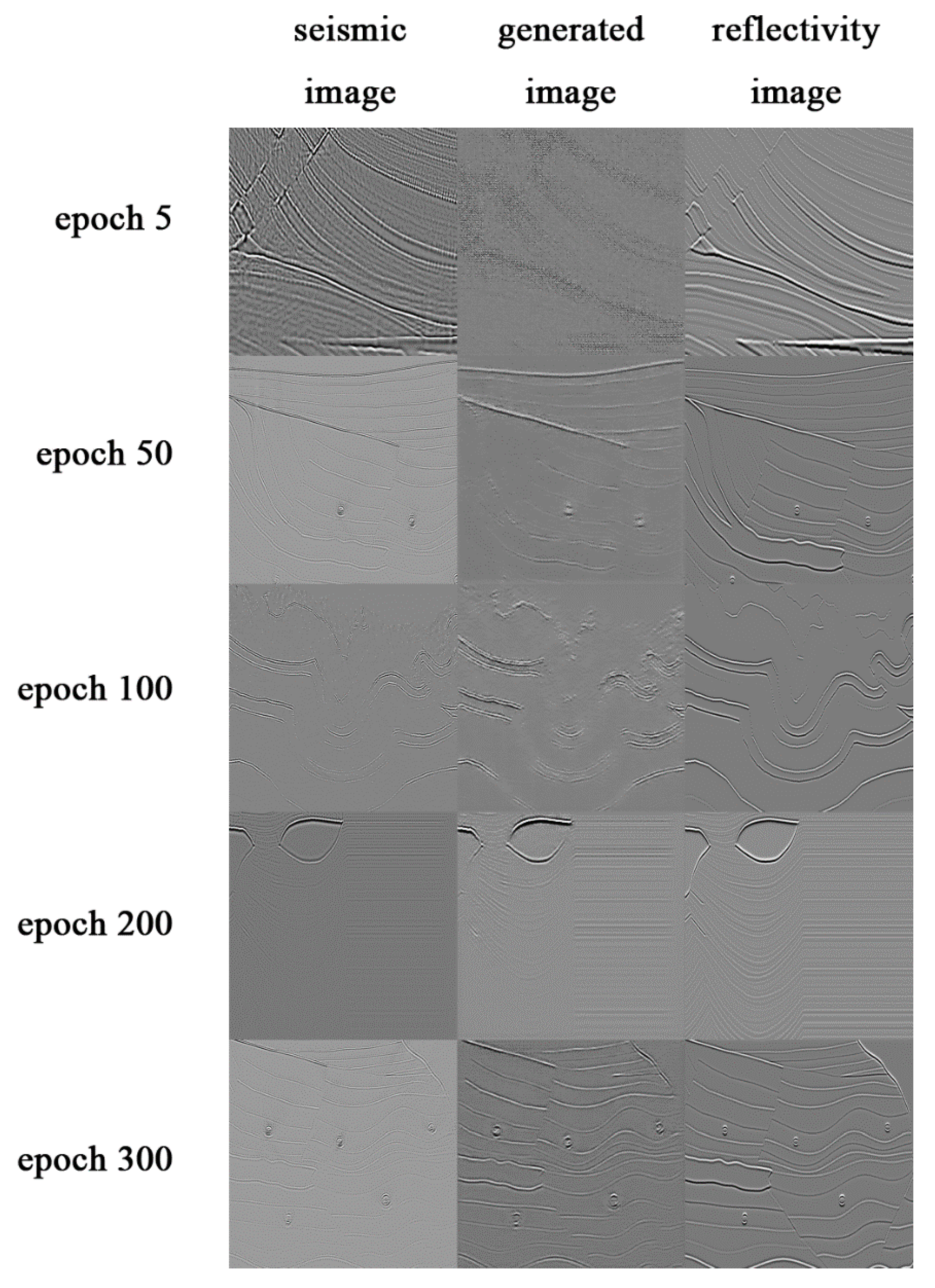
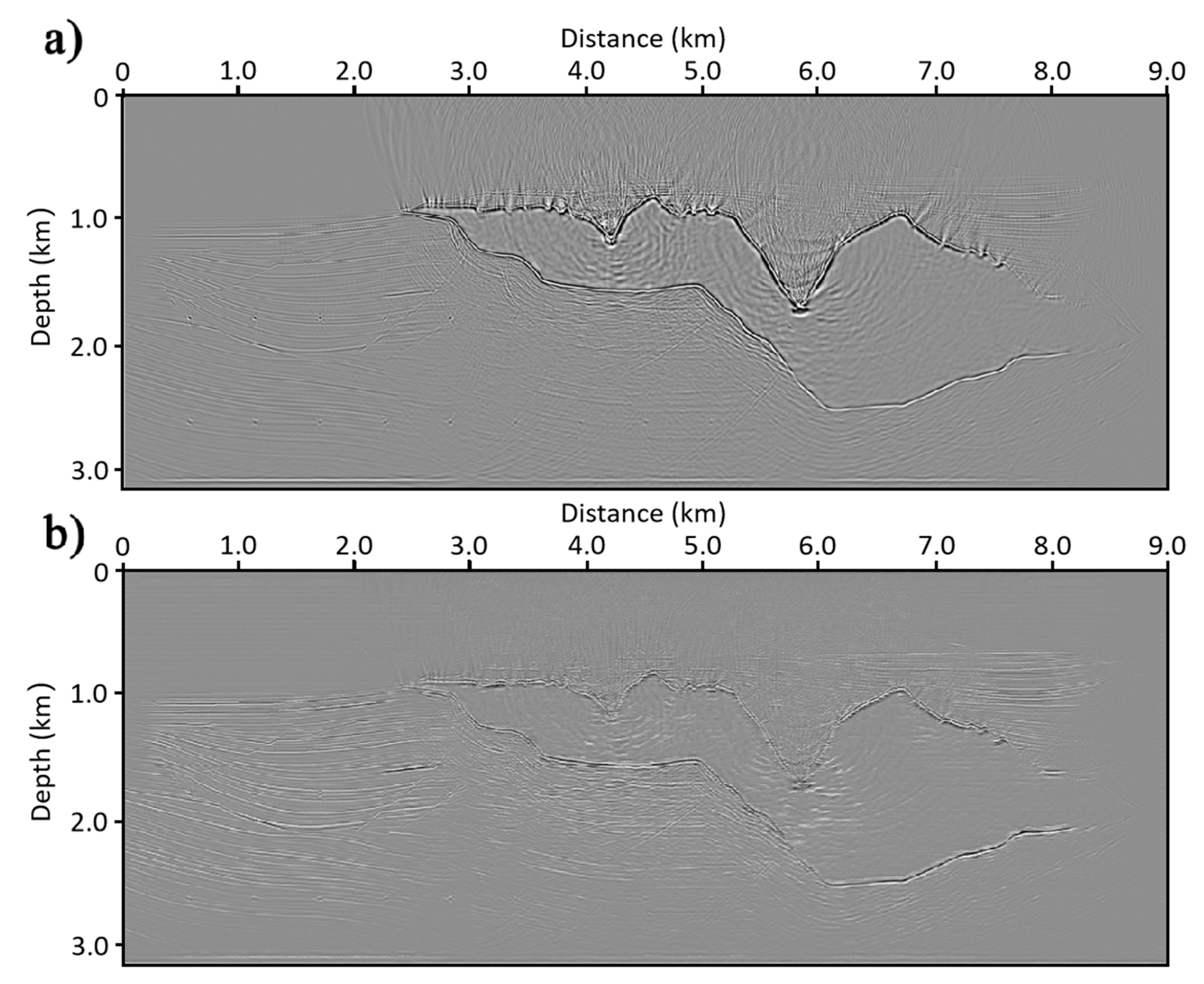
The structure similarity index (SSIM) is a classical method for measuring perceptual quality [51]. We used the SSIM to measure the similarity between the generated images and the real images. The SSIM evaluates the similarity of the images from three perspectives: luminance, contrast, and structure. The SSIM can be formulated as

$$SSIM(x,y)=\frac{(2{\mu }_x{\mu }_y+c_1)(2{\sigma }_{xy}+c_2)}{({\mu }_x{}^2{\mu }_y{}^2+c_1)({\mu }_x{}^2{\mu }_y{}^2+c_2)}$$

(4)

where ${\mu }_x,{\mu }_y$ are the averages of the images, ${\sigma }_x{}^2,{\sigma }_y{}^2$ are the variances of x and y, ${\sigma }_{xy}$ is the covariance of x and y, and $c_1,c_2$ are two variables to stabilize the division with a weak denominator.

The SSIM function is symmetrical: $SSIM(x,y)=SSIM(y,x)$. The value range of the SSIM is from 0 to 1, and $SSIM(x,y)=1$ is reached only when the two input images are identical.

9. Examples

The deep learning programming framework we used was PyTorch, and the training was performed on an Nvidia Quadro RTX 6000 graphics device. We used 6 classical synthetic seismic models (foothill model, Hess model, Marmousi model, Pluto model, BGP-salt, and Sigsbee model) to train and evaluate the conditional GAN, and the properties of the datasets are shown in

Table 1. The properties of the training datasets. There were 6 models (foothill, Hess, BGP-salt, Marmousi, Pluto, and Sigsbee) in the dataset. The first 5 models were used as the training dataset, and the Sigsbee model was used as the validation dataset.

Model Name	Model Size	RTM Method
foothill	1568 × 900	Grid method
Hess	3617 × 1500	Grid method
BGP-salt	3000 × 1400	Grid method
Marmousi	2181 × 751	Finite difference
Pluto	6960 × 1201	Finite difference
Sigsbee	3201 × 1201	Finite difference

. Special geological structure properties such as high-dip-angle reflection, the overthrust structure, surface topography, salt bodies, and scattering points are included in the training dataset. We used the Sigsbee model as the validation data. The Sigsbee dataset was modeled by simulating the geological setting found on the Sigsbee Escarpment in the deep-water Gulf of Mexico. The model highlights the illumination problems caused by the complex salt shape of the rugose salt top found in this area. The rugged surface of a salt top is an important source of imaging noise. The imaging noise problem in these data is typical, so we used these data as the validation dataset to verify the feasibility of the method, and the remaining five models were used as the training data.

In each training epoch, we randomly cropped 32 images with a size of 256 × 256 from the training dataset and adopted data augmentation before feeding them into the conditional GAN. Data augmentation is one of the commonly used techniques in deep learning. It is mainly used to increase the size of the training dataset, make the dataset as diverse as possible, and help the training model to develop stronger generalization ability. In practical application, in order to increase the number of training samples, we often manipulate the data by flipping, mirroring, rotating, etc., before feeding them to the neural network. Due to the network’s structure, especially the shortcut feature, when the dataflow passes through the bottleneck layer in the middle of the network, the process is then reversed. One advantage of a fully connected neural network model is that the input size of the image is unrestricted. Thus, we can input an image of arbitrary size without modifying the architecture. For an image translation task, it is necessary to maintain lots of low-level information. An efficient method is to shuttle the low-level information across the network. U-net adopts a skip connection between each layer $\mathrm{i}$ and layer $\mathrm{n}-\mathrm{i}$, where $\mathrm{n}$ is the depth of U-net. As a result, U-net has proved to be effective on a small dataset while avoiding overfitting. Thus, the “small training data” are able to finish the task. The training epoch was 12,000, and several intermediate training results are shown in Figure 7. As can be seen in Figure 7, the GAN begins by learning the structure of the image. Then, the details are learned step by step. After about 300 epochs, the generator can depict the fine structure of the image.

The losses are plotted in Figure 8. As can be seen in this figure, the losses converged to a steady state progressively. $L_{GAN}$ and $L_1$ decreased while $L_D$ increased in the long term. After about 4000 epochs, the training process converged when the loss function became stable.

Both the U-net generator and the Markovian discriminator adopted are FCN models, which do not require an input model of a fixed size. The generator works when both the width and the height are a multiple of 256. To satisfy the requirement of the generator, we performed zero padding. Thus, we were able to put the whole image into the generator and obtain the denoised image at one time. In this way, the image-stitching problem is naturally solved. We used the Sigsbee model to validate the generalization performance of the GAN.

As Figure 9 shows, the structure was undistorted, and the noise was largely suppressed, especially the noise near shots. In addition, the SSIM increased from $SSIM(y,x)=0.47$ to $SSIM(G(z|y),x)=0.66$, indicating that the GAN method has preliminary potential for addressing the problem of denoising seismic imaging.

10. Conclusions

In this work, we proposed a conditional GAN method for imaging domain denoising. The method was developed based on a deblur GAN. We adopted the pix2pix GAN architecture and the WGAN-GP as the objective function. Through the experiment, we showed that the training process converged progressively owing to the robust WGAN-GP objective function. Furthermore, we demonstrated that our method could, in one go, maintain the structure of the seismic image while suppressing different types of noise in the seismic image. Using the Sigsbee model, we validated the generalization ability of the trained GAN. The SSIM index further proved the feasibility of our method.

References

1. Liu, W.; Chen, W. Recent advancements in empirical wavelet transform and its applications. IEEE Access 2019, 7, 103770–103780. [Google Scholar] [CrossRef]
2. Siahsar, M.A.N.; Abolghasemi, V.; Chen, Y. Simultaneous denoising and interpolation of 2D seismic data using data-driven non-negative dictionary learning. Signal Process. 2017, 141, 309–321. [Google Scholar] [CrossRef]
3. Yilmaz, Ö.; Tanir, I.; Gregory, C.; Zhou, F. Interpretive imaging of seismic data. Lead. Edge 2001, 20, 132–144. [Google Scholar] [CrossRef]
4. Chen, Y.; Fomel, S. Random noise attenuation using local signal-and-noise or- thogonalization. Geophysics 2015, 80, WD1–WD9. [Google Scholar] [CrossRef]
5. Liu, G.; Chen, X.; Du, J.; Wu, K. Random noise attenuation using f-x regularized nonstationary autoregression. Geophysics 2012, 77, V61–V69. [Google Scholar] [CrossRef]
6. Naghizadeh, M.; Sacchi, M.D. Multicomponent seismic random noise attenuation via vector autoregressive operators. Geophysics 2012, 77, V91–V99. [Google Scholar] [CrossRef]
7. Gan, S.; Wang, S.; Chen, Y.; Chen, X.; Xiang, K. Separation of simultaneous sources using a structural-oriented median filter in the flattened dimension. Comput. Geosci. 2016, 86, 46–54. [Google Scholar] [CrossRef]
8. Liu, G.; Chen, X. Noncausal f−x−y regularized nonstationary prediction filtering for random noise attenuation on 3D seismic data. J. Appl. Geophys. 2013, 93, 60–66. [Google Scholar] [CrossRef]
9. Liu, Y. Noise reduction by vector median filtering. Geophysics 2013, 78, V79–V87. [Google Scholar] [CrossRef]
10. Fomel, S.; Liu, Y. Seislet transform and seislet frame. Geophysics 2010, 75, V25–V38. [Google Scholar] [CrossRef] [Green Version]
11. Mousavi, S.M.; Langston, C.A.; Horton, S.P. Automatic microseismic denoising and onset detection using the synchrosqueezed continuous wavelet transform. Geophysics 2016, 81, V341–V355. [Google Scholar] [CrossRef]
12. Zu, S.; Zhou, H.; Ru, R.; Jiang, M.; Chen, Y. Dictionary learning based on dip patch selection training for random noise attenuation. Geophysics 2019, 84, V169–V183. [Google Scholar] [CrossRef]
13. Huang, W.; Wang, R.; Chen, Y.; Li, H.; Gan, S. Damped multichannel singular spectrum analysis for 3D random noise attenuation. Geophysics 2016, 81, V261–V270. [Google Scholar] [CrossRef]
14. Oropeza, V.; Sacchi, M. Simultaneous seismic data denoising and reconstruction via multichannel singular spectrum analysis. Geophysics 2011, 76, V25–V32. [Google Scholar] [CrossRef]
15. Lecun, Y.; Bengio, Y.; Hinton, G. Deep learning. Nature 2015, 521, 436–444. [Google Scholar] [CrossRef] [PubMed]
16. Krizhevsky, A.; Sutskever, I.; Hinton, G.E. ImageNet classification with deep convolutional neural networks. Commun. ACM 2017, 60, 84–90. [Google Scholar] [CrossRef]
17. Ronneberger, O.; Fischer, P.; Brox, T. U-net: Convolutional networks for biomedical image segmentation. In Proceedings of the18th International Conference, Munich, Germany, 5–9 October 2015; Lecture Notes in Computer Science (Including Subseries Lecture Notes in Artificial Intelligence and Lecture Notes in Bioinformatics);. Volume 9351, pp. 234–241. [Google Scholar]
18. Zhang, K.; Zuo, W.; Gu, S.; Zhang, L. Learning Deep CNN Denoiser Prior for Image Restoration. In Proceedings of the IEEE Conference on Computer Vision and Pattern, Honolulu, HI, USA, 21–26 July 2017; pp. 3929–3938. [Google Scholar]
19. Long, J.; Shelhamer, E.; Darrell, T. Fully convolutional networks for semantic segmentation. In Proceedings of the 2015 IEEE Conference on Computer Vision and Pattern Recognition (CVPR), Boston, MA, USA, 7–12 June 2015; Volume 31, pp. 3431–3440. [Google Scholar]
20. Yuan, S.; Liu, J.; Wang, S.; Wang, T.; Shi, P. Seismic Waveform Classification and First-Break Picking Using Convolution Neural Networks. IEEE Geosci. Remote Sens. Lett. 2018, 15, 272–276. [Google Scholar] [CrossRef]
21. Wu, X.M.; Liang, L.; Shi, Y.; Fomel, S. FaultSeg3D: Using synthetic data sets to train an end-to-end convolutional neural network for 3D seismic fault segmentation. Geophysics 2019, 84, IM35–IM45. [Google Scholar] [CrossRef]
22. Xiong, W.; Ji, X.; Ma, Y.; Wang, Y.; AlBinHassan, N.; Ali, M.; Luo, Y. Seismic fault detection with convolutional neural network. Geophysics 2018, 83, O97–O103. [Google Scholar] [CrossRef]
23. Lewis, W.; Vigh, D. Deep learning prior models from seismic images for full-waveform inversion. In SEG Technical Program Expanded Abstracts 2017; Society of Exploration of Geophysicists: Houston, TX, USA, 2017; pp. 1512–1517. [Google Scholar]
24. Shi, Y.; Wu, X.; Fomel, S. Automatic salt-body classification using deep-convolutional neural network. In SEG Technical Program Expanded Abstracts 2018; Society of Exploration of Geophysicists: Anaheim, CA, USA, 2018; pp. 1971–1975. [Google Scholar]
25. Zhang, Y.; Liu, Y.; Zhang, H.; Xue, H. Seismic facies analysis based on deep learning. IEEE Geosci. Remote Sens. Lett. 2019, 17, 1119–1123. [Google Scholar] [CrossRef]
26. Jin, Y.; Wu, X.; Chen, J.; Han, Z.; Hu, W. Seismic Data Denoising by Deep Residual Networks. In SEG Technical Program Expanded Abstracts 2018; Society of Exploration of Geophysicists: Anaheim, CA, USA, 2018; pp. 4593–4597. [Google Scholar]
27. Sang, W.J.; Yuan, S.Y.; Yong, X.S.; Jiao, X.Q.; Wang, S.X. DCNNs-Based Denoising With a Novel Data Generation for Multidimensional Geological Structures Learning. IEEE Geosci. Remote Sens. Lett. 2021, 18, 1861–1865. [Google Scholar] [CrossRef]
28. Yuan, S.; Jiao, X.; Luo, Y.; Sang, W.; Wang, S. Double-scale supervised inversion with a data-driven forward model for low-frequency impedance recovery. Geophysics 2022, 87, R165–R181. [Google Scholar] [CrossRef]
29. Wang, W.; Ma, J. Velocity model building in a crosswell acquisition geometry with image-trained artificial neural networks. Geophysics 2020, 85, U31–U46. [Google Scholar] [CrossRef]
30. Woollam, J.; Rietbrock, A.; Bueno, A.; De Angelis, S. Convolutional Neural Network for Seismic Phase Classification, Performance Demonstration over a Local Seismic Network. Seismol. Res. Lett. 2019, 90, 491–502. [Google Scholar] [CrossRef]
31. Zhang, H.; Han, J.G.; Li, Z.X.; Zhang, H. Extracting Q Anomalies from Marine Reflection Seismic Data Using Deep Learning. IEEE Geosci. Remote Sens. Lett. 2022, 19, 7501205. [Google Scholar] [CrossRef]
32. Goodfellow, I.J.; Pouget-Abadie, J.; Mirza, M.; Xu, B.; Warde-Farley, D.; Ozair, S.; Courville, A.; Bengio, Y. Generative Adversarial Networks. arXiv 2014, arXiv:1406.2661. [Google Scholar] [CrossRef]
33. Li, Y.; Xiao, N.; Ouyang, W. Improved boundary equilibrium generative adversarial networks. IEEE Access 2018, 6, 11342–11348. [Google Scholar] [CrossRef]
34. Mao, X.; Li, Q.; Xie, H.; Lau, R.Y.K.; Wang, Z.; Smolley, S.P. Least Squares Generative Adversarial Networks. In Proceedings of the IEEE International Conference on Computer Vision (ICCV), Venice, Italy, 22–29 October 2017; pp. 2794–2802. [Google Scholar]
35. Radford, A.; Metz, L.; Chintala, S. Unsupervised Representation Learning with Deep Convolutional Generative Adversarial Networks. arXiv 2015, arXiv:1511.06434. [Google Scholar]
36. Mirza, M.; Osindero, S. Conditional Generative Adversarial Nets. arXiv 2014, arXiv:1411.1784. [Google Scholar]
37. Ledig, C.; Theis, L.; Huszár, F.; Caballero, J.; Cunningham, A.; Acosta, A.; Aitken, A.; Tejani, A.; Totz, J.; Wang, Z.; et al. Photo-realistic single image super-resolution using a generative adversarial network. In Proceedings of the 30th IEEE Conference on Computer Vision and Pattern Recognition, CVPR 2017, Honolulu, HI, USA, 21–26 July 2017; pp. 105–114. [Google Scholar]
38. Kupyn, O.; Budzan, V.; Mykhailych, M.; Mishkin, D.; Matas, J. DeblurGAN: Blind Motion Deblurring Using Conditional Adversarial Networks. In Proceedings of the IEEE Conference on Computer Vision and Pattern Recognition, Salt Lake City, UT, USA, 18–23 June 2018; pp. 8183–8192. [Google Scholar]
39. Isola, P.; Zhu, J.Y.; Zhou, T.; Efros, A.A. Image-to-image translation with conditional adversarial networks. In Proceedings of the 30th IEEE Conference on Computer Vision and Pattern Recognition, CVPR 2017, Honolulu, HI, USA, 21–26 July 2017; pp. 5967–5976. [Google Scholar]
40. Maas, A.L.; Hannun, A.Y.; Ng, A.Y. Rectifier nonlinearities improve neural network acoustic models. In Proceedings of the 30th International Conference on Machine Learning, ICML’13, Atlanta, GA, USA, 16–21 June 2013. [Google Scholar]
41. Ulyanov, D.; Vedaldi, A.; Lempitsky, V. Instance Normalization: The Missing Ingredient for Fast Stylization. arXiv 2016, arXiv:1607.08022. [Google Scholar]
42. Zeiler, M.D.; Taylor, G.W.; Fergus, R. Adaptive Deconvolutional Networks for Mid and High Level Feature Learning. In Proceedings of the IEEE International Conference on Computer Vision, Barcelona, Spain, 6–13 November 2011; pp. 2018–2025. [Google Scholar]
43. Nair, V.; Hinton, G.E. Rectified Linear Units Improve Restricted Boltzmann Machines. In Proceedings of the 27th International Conference on Machine Learning (ICML’10), Haifa, Israel, 21–24 June 2010. [Google Scholar]
44. Hinton, G.E.; Srivastava, N.; Krizhevsky, A.; Sutskever, I.; Salakhutdinov, R.R. Improving neural networks by preventing co-adaptation of feature detectors. arXiv 2012, arXiv:1207.0580v1. [Google Scholar]
45. Son, J.; Park, S.J.; Jung, K.-H. Retinal Vessel Segmentation in Fundoscopic Images with Generative Adversarial Networks. arXiv 2017, arXiv:1706.09318. [Google Scholar]
46. Yang, P.; Gao, J.; Wang, B. RTM using effective boundary saving: A staggered grid GPU implementation. Comput. Geosci. 2014, 68, 64–72. [Google Scholar] [CrossRef]
47. Liu, Q.; Zhang, J.; Gao, H. Reverse-time migration from rugged topography using irregular, unstructured mesh. Geophys. Prospect. 2017, 65, 453–466. [Google Scholar] [CrossRef]
48. Gulrajani, I.; Ahmed, F.; Arjovsky, M.; Dumoulin, V.; Courville, A. Improved Training of Wasserstein GANs. arXiv 2017, arXiv:1704.00028. [Google Scholar]
49. Arjovsky, M.; Chintala, S.; Bottou, L. Wasserstein GAN. arXiv 2017, arXiv:1701.07875. [Google Scholar]
50. Kingma, D.P.; Ba, J. Adam: A Method for Stochastic Optimization. arXiv 2014, arXiv:1412.6980. [Google Scholar]
51. Wang, Z.; Bovik, A.C.; Sheikh, H.R.; Member, S.; Simoncelli, E.P.; Member, S. Image Quality Assessment: From Error Visibility to Structural Similarity. IEEE Trans. Image Process. 2004, 13, 600–612. [Google Scholar] [CrossRef] [Green Version]
Figure 1. The architecture of a conditional GAN. A conditional GAN has two DNNs: a generator G and a discriminator D . The generator creates the conditional image synthesis, and the discriminator calculates the conditional distance between the generated objects and the real ones.
Energies 15 06569 g001
Figure 2. The architecture of the U-net generator. U-net is named for its U-shaped network architecture, and it is an end-to-end encoder–decoder model for semantic segmentation. We followed the U-net configuration in the pix2pix GAN. The network has 16 layers, with an 8-layer encoder and an 8-layer decoder. See the text for detailed information.
Energies 15 06569 g002
Figure 3. The architecture of the Markovian discriminator (also known as the patch GAN). It is a 5-layer FCN model for discriminating texture loss. It assumes that the independence between pixels is greater than a patch diameter and regards the image as a Markov random field. The Markovian discriminator runs in a convolutional way across the image, each time penalizing a part of the image at the patch scale. The ultimate output of the discriminator is the average of all responses of the patches.
Energies 15 06569 g003
Figure 4. The image pairs “AB” for training. The images on the left are the seismic images “A”, and the images on the right are the reflectivity images “B”. The “A” images were derived through the RTM migration technique, and the “B” images were derived through the precise velocity model.
Energies 15 06569 g004
Figure 5. The training process of a conditional GAN. The generator creates a restored image G ( z | y ) from z on the condition of y . The discriminator is trained by feeding it the denoised image x and the seismic image y . The generator and the discriminator have different loss functions and are trained iteratively.
Energies 15 06569 g005
Figure 6. The workflow of the conditional GAN training. First, train the discriminator for n c r i t i c times and update the parameters of the discriminator. In our experiment, n c r i t i c = 5 . Second, train the generator and update the generator parameters depending on the updated discriminator parameters. The two steps iterate until the generator converges to a stable state.
Energies 15 06569 g006
Figure 7. The intermediate results in the process of training. The GAN begins by learning the structure of the image. Then, the details are learned step by step. After about 300 epochs, the generator can depict the fine structure of the image.
Energies 15 06569 g007
Figure 8. The loss curves. As can be seen in this figure, the losses converged to a steady state progressively. L G A N and L 1 decreased while L D increased in the long term. After about 4000 epochs, the training process became stable.
Energies 15 06569 g008
Figure 9. (a) The migration image of the Sigsbee model, and (b) the denoised Sigsbee model produced by the generator. As can be seen, the structure was undistorted, and the noise was largely suppressed, especially the noise between the surface and the rugged surface of the salt top.
Energies 15 06569 g009