Article

Investigations of Vertical-Axis Wind-Turbine Group Synergy Using an Actuator Line Model

Mechanical and Mechatronics Engineering, University of Waterloo, 200 University Avenue West, Waterloo, ON N2L 3G1, Canada
*
Author to whom correspondence should be addressed.
Energies 2022, 15(17), 6211; https://doi.org/10.3390/en15176211
Submission received: 15 August 2022 / Revised: 23 August 2022 / Accepted: 24 August 2022 / Published: 26 August 2022
(This article belongs to the Special Issue Vertical-Axis Wind Turbine)

Abstract

:
The presence of power augmentation effects, or synergy, in vertical-axis wind turbines (VAWTs) offers unique opportunities for enhancing wind-farm performance. This paper uses an open-source actuator-line-method (ALM) code library for OpenFOAM (turbinesFoam) to conduct an investigation into the synergy patterns within two- and three-turbine VAWT arrays. The application of ALM greatly reduces the computational cost of simulating VAWTs by modelling turbines as momentum source terms in the Navier–Stokes equations. In conjunction with an unsteady Reynolds-Averaged Navier–Stokes (URANS) approach using the k- ω shear stress transport (SST) turbulence model, the ALM has proven capable of predicting VAWT synergy. The synergy of multi-turbine cases is characterized using the power ratio which is defined as the power coefficient of the turbine cluster normalized by that for turbines in isolated operation. The variation of the power ratio is characterized with respect to the array layout parameters, and connections are drawn with previous investigations, showing good agreement. The results from 108 two-turbine and 40 three-turbine configurations obtained using ALM are visualized and analyzed to augment the understanding of the VAWT synergy landscape, demonstrating the effectiveness of various layouts. A novel synergy superposition scheme is proposed for approximating three-turbine synergy using pairwise interactions, and it is shown to be remarkably accurate.

1. Introduction

Wind energy is a vital element in creating a sustainable energy future, and wind turbines is a thriving area for contemporary research. Horizontal-axis wind turbines (HAWTs) and vertical-axis wind turbines (VAWTs) are two mature technologies available today for wind-energy extraction, though the former is adopted almost universally and occupies the vast majority of the market share [1]. In this area, Liu et al. [2] performed a fluid-structure interaction study on a novel hybrid Darrieus-Modified-Savonius VAWT design, Jain & Abhishek [3] comprehensively investigated the impact of turbine parameters on the performance of a VAWT with dynamic blade pitching, Johari et al. [4] conducted an experimental comparison of the performances of a small-scale HAWT and VAWT, Du et al. [5] provided an extensive review of H-Darrieus VAWT literature, and Ghasemian et al. [6] reviewed computational fluid dynamic (CFD) simulation techniques for Darrieus VAWTs. From these works, the comparative disadvantages of the VAWTs are identified to be lower aerodynamic efficiencies [2,3,4], self-starting issues encountered at lower wind speeds [2,3,5,6], and structural difficulties in large-scale designs [1]. These shortcomings notwithstanding, the VAWT archetype remains interesting to study and refine because of its unique, intrinsic properties: namely, operational feasibility at smaller scales [3,7] and omni-directional power generation [8]. Such traits confer on VAWTs higher suitability for operation in distributed energy settings such as urban areas, where low-noise requirements and robustness to volatile wind directions restrict the utilization of HAWTs. As a consequence, it is this applicability that continues to drive research on this subject, with efforts to augment the power performance of VAWTs directed towards unique turbine/blade designs [2], guide vanes [6,9], blade-pitch control [10,11,12], and intra-cycle rotational speed control [13].
Recent discoveries within the last decade have demonstrated the additional benefits of the VAWT. Experimental investigations conducted by Kinzel et al. [14] found that the stream-wise velocity could recover to 95% of the freestream at only 6D (where D is the rotor diameter) downstream of a VAWT, compared to some 14D required by a HAWT. This essentially enables tighter array packing within wind farms, while still mitigating the detrimental effects of turbine wakes on power generation. In 2010, Dabiri [7] found that H-bladed Darrieus VAWTs operating in close proximity to one another exhibited larger power coefficients ( C P ) than their isolated equivalents, revealing the existence of a mutually beneficial, power-enhancing phenomenon driven by inter-turbine interaction. We refer to this favorable effect as “synergy” in this work for conciseness, as this term has been adopted in prior literature (e.g., by Hezaveh et al. [15]).
Subsequent works, both experimental and numerical, have confirmed the presence of synergy. Ahmadi-Baloutaki et al. [16] tested two- and three-turbine arrays in wind tunnel experiments, finding synergy both among adjacent pairs (turbines placed side-by-side perpendicular to the incident wind direction) and among staggered configurations. Zanforlin & Nishino [17] studied synergy in a pair of VAWTs using the unsteady Reynolds-Averaged Navier–Stokes (URANS) approach with a k- ω shear stress transport (SST) turbulence model, establishing a precedent for using numerical methods and turbulence models to model synergy. Lam & Peng [18] confirmed the presence of synergy by measuring the wake characteristics of a pair of VAWTs and proposed the idea that small synergistic clusters (composed of 2 and/or 3 turbines) can be used as building blocks when optimizing placement in a larger wind farm. Peng [19] used a dynamic torque-driven approach (in contrast to the more commonly prescribed rotational velocity approach) to model the operation of VAWTs and determined that an array of five turbines could still manifest synergy. Shaaban et al. [20] and Barnes & Hughes [21] used URANS coupled with a turbulence model to study synergy among arrays consisting of up to 6 and 16 turbines, respectively. Brownstein et al. [22] performed a detailed experimental characterization of the 3-D flow field surrounding pairs of VAWTs, establishing synergy patterns such as the degradation of a downwind turbine’s performance as it enters an upwind turbine’s wake. In 2021, Hansen et al. [23] performed a comprehensive study of synergy in two- and three-turbine arrays by parameterizing configurations using the relative angle and spacing, thereby contributing valuable insight on the functional relationship between turbine positioning and synergy.
The implication of this abundantly supported synergy phenomenon is the unprecedented opportunity to arrange VAWTs closer together in order to produce greater power, a concept unthinkable for HAWTs. As a consequence, it is of crucial importance to model synergistic effects in large VAWT farms to exploit this feature as part of micro-siting and optimization efforts. For these applications, the conventional full-order or blade-resolved computational fluid dynamics (CFD) of VAWTs using URANS [24,25,26,27,28] or large-eddy simulation (LES) [10,29,30], in which blade-level dynamics are explicitly resolved in the mesh, can be prohibitively expensive at the wind-farm scale. Therefore, the development of reduced-order models involving various forms of approximations or simplifications can become invaluable for wind-farm-level modelling. Sanderse et al. [31] surveyed the pertinent literature to find that the common approaches are momentum-based streamtube models, free/fixed vortex models, and actuator models. Delafin et al. [32] compared the accuracy of a Double Multiple Streamtube (DMST) model, a free-vortex model, and a full-order CFD model, finding that the reduced-order models led to significant errors. The actuator models are more robust, since they are used in conjunction with CFD and can employ a variety of representations for the rotor/blades, such as the actuator disk model [31], the actuator surface or cylinder model [30,33], and the actuator line model [34]. Among these, the Actuator Line Model (ALM) enables the highest fidelity approximation, owing to the fact that the blade motion being dynamically incorporated in the solver [31,34]. This accuracy advantage is saliently demonstrated in a comparison of the Actuator Swept-Surface Model (ASSM) and the ALM performed by Shamsoddin & Porté-Agel [30]. As a result, we chose to explore the capabilities of the ALM in the context of the prediction and characterization of VAWT synergy.
Originally, the ALM was developed by Sørensen & Shen [35] in 2002 to model HAWT performance. In this formulation, blade-element momentum (BEM) theory describes the forces acting on blade elements as a function of the local relative velocity ( u r e l ), the angle of attack ( α ), and the lift and drag coefficients ( C l and C d , respectively) obtained from airfoil data tables. These blade forces are then reversed and applied to the flow field as momentum source terms to the Navier–Stokes equations after being smoothed by a Gaussian regularization kernel ( η ) to avoid singularity effects [35]. In recent years, researchers have applied ALM to the modelling of VAWTs by adapting the formulation while maintaining the underlying theory. Shamsoddin & Porté-Agel [30], Hezaveh et al. [36], Creech et al. [37], and Abkar [38] are important investigations that use ALM and LES to study VAWT-wake characteristics and performance, typically with an emphasis on the former. While the results of these investigations crucially demonstrate the applicability of ALM to VAWTs, the LES studies broadly feature coarse grids (often with a cell size far greater than the blade chord) and time-averaging and thus do not prioritize the simulations of the blade-level dynamics. The seminal works of Bachant et al. [39] and Zhao et al. [34] demonstrated that a reduced-order approach consisting of ALM and URANS (with a turbulence model) is both valid and promising for future VAWT investigations. Some recent studies focus on enhancing the fidelity of VAWT ALM (with LES and URANS) by using cubic spline smoothing on the angle of attack combined with a novel inflow velocity sampling procedure [40], evaluating advanced sub-models for tip effects (Glauert correction versus Dag & Sørensen) [41], and developing a cohesive and upgraded framework to account for higher-order aerodynamic effects [42].
To our best knowledge, there are only two published investigations that apply VAWT ALM to the study of wind turbine array synergy: namely, Hezaveh et al. [15] in 2018 and Raj V et al. [43] in 2021. While it is a groundbreaking approach that leverages the computational efficiency of ALM to investigate synergy, the ALM-LES study by Hezaveh et al. [15] utilizes a grid size relative to the blade chord length (c) of 2.22 c (implying significant spatial averaging) and does not validate the aerodynamic forces to prove synergy. Raj V et al. [43] used ALM and URANS to confirm that the coefficients of power for VAWTs in a two-turbine configuration exceed that of isolated rotors. The use of ALM-LES in the study of VAWTs is standard practice, since LES can directly resolve most of the turbulent energy spectrum and compute small-scale dynamics using a subgrid-scale (SGS) model. According to Bachant et al. [39], this enables the capture of the important mean swirling motion near the turbine, as well as the turbulence effects produced by the blade–tip vortex shedding and dynamic stall. However, while, in theory, ALM-LES is the superior approach given a sufficiently fine grid resolution, such a case could be prohibitively expensive. For example, Bachant et al.’s [39] ALM-LES simulation with the UNH-RVAT turbine utilizes a reasonably refined grid consisting of 64 cells per turbine diameter but requires 100 times the computational effort of an ALM-URANS simulation that is similarly refined. As a consequence, there is potential for ALM-URANS to offer a more cost-effective solution to the modelling of VAWT synergy while achieving reasonable accuracy, even though turbulence phenomena would be less accurately resolved relative to ALM-LES. The 3-D full-order or blade-resolved CFD results are significantly more expensive, with a 3-D full-order URANS simulation being four orders of magnitude more expensive computationally than ALM-URANS [39], and LES simulations would be even more computationally costly. Given this context, we seek to contribute value to the current research landscape by applying ALM-URANS to the study of a wide variety of two- and three-turbine configurations in order to characterize the fundamental patterns that arise from the emergence and magnitude of VAWT synergy.
Following this Introduction, in Section 2, we present the ALM formulation (Section 2.1), the turbine geometry and CFD parameters (Section 2.2), the two-turbine group-configuration design (Section 2.3), the three-turbine group configuration design (Section 2.4), and our novel synergy superposition scheme (Section 2.5). In Section 3, we start with a validation of the presently used ALM approach using results from various methodologies/sources (Section 3.1) and then present the two-turbine group results (Section 3.2), three-turbine group results (Section 3.3), the effectiveness of the synergy superposition scheme (Section 3.4), and the key conclusions of our investigations (Section 4).

2. Methodology

2.1. Actuator Line Model Formulation

We use the open-source ALM library developed by Bachant et al. [39] for OpenFOAM (referred to as turbinesFoam [44]), to perform the ALM-URANS calculations. This library grants ease-of-access to researchers aiming to implement vertical-axis (wind) turbine ALM in a computationally performative manner, and it is easily extendable to multi-turbine simulations. In the original work of Bachant et al. [39], this framework is validated using experimental results for the UNH-RVAT and RM2 turbines, showing particularly good agreement in terms of C P versus the tip-speed ratio (or TSR, which is defined as the rotor-tip speed divided by the freestream-incident wind speed) in the former case. Mendoza et al. [45] utilized this library in an ALM-LES study that established high degrees of accuracy in the cyclic variations of the angle of attack and rotor normal force compared to experiments. Mendoza & Goude [46] compared the ALM-LES approach to two different vortex models and some experimental measurements, also demonstrating good agreement with the measured normal forces. Therefore, the validity of this formulation and the correctness of the code implementation have been consistently demonstrated through these works.
In the current section, we will provide a brief summary of the mathematical formulation of Bachant et al.’s [39] ALM implementation. Each blade in the turbine is discretized in the span-wise direction into actuator elements (blade elements), and each element is assigned a control point (the actuator point) located at the mid-span and the quarter-chord location within the element. Each actuator point governs the forces for the entire associated actuator element. Figure 1 shows a sample blade element rotating with angular velocity ω in the counterclockwise (CCW) direction due to an incident wind in the positive x-direction. The blade is fixed along a circular trajectory at a distance R (corresponding to the rotor radius) from the center of the turbine, with the mounting point being the quarter-chord location or actuator point. The azimuthal angle θ of the blade is defined as the CCW starting from the positive x-axis and varies due to the constant rotational velocity ω . The blade’s rotation induces a relative velocity of ω R in the trajectory’s tangential direction, and the blade also experiences the local flow vector u (which is predominantly comprised of the stream-wise component). Thus, the relative velocity u r e l at the actuator point is the vector difference between ω R and u . Once obtained, u r e l determines the angle of attack, α , along with the lift and drag forces ( F l and F d , respectively) experienced by this actuator element. At an appropriate, chord-based Reynolds number, R e c , α is used to look up the sectional airfoil aerodynamic coefficients ( C l and C d ) sourced from the Sheldahl & Klimas [47] report. At this stage, the forces can be computed as follows [39]:
F l = 1 2 ρ A e l e m C l | u r e l | 2 ,
F d = 1 2 ρ A e l e m C d | u r e l | 2 ,
where ρ is density of the air, A e l e m is the blade element planform area (span times chord), and u r e l is the local relative velocity.
After these forces are obtained and converted into the desired components (viz. the force components along x-y Cartesian coordinate directions), they are convolved with an isotropic, three-dimensional (3-D) Gaussian regularization kernel at each cell neighboring the actuator point in order to distribute and smooth the forces. The Gaussian kernel used assumes the following form:
η = 1 ϵ 3 π 3 / 2 exp | r | ϵ 2 ,
where η is the kernel value (calculated individually for every relevant cell), ϵ is the Gaussian width (controlling the central concentration of the force distribution), and | r | is the distance from the actuator point to the cell centroid. The ϵ parameter can be tuned to obtain a kernel that most accurately captures the actual blade dynamics. To this purpose, Bachant et al. [39] uses the maximum of three values, which are based on chord length, mesh size, and the momentum thickness due to drag, to determine ϵ . In practice, the property that determines the value of ϵ is the mesh size, namely, ϵ = 2 C m e s h Δ x , where C m e s h = 2 is a calibration factor, and Δ x is the approximate cell size (cube root of the cell volume). At each cell, within some threshold radius of the actuator point, the cell-specific η is multiplied with the forces to perform the projection. This threshold radius is set to be c + ϵ ( ln ( 1.0 / 0.001 ) ) 1 / 2 [44], which encapsulates a sufficiently high percentage of the total (probability) mass of the kernel in the present cases. This means the corresponding percentage of the forces at the actuator point can be distributed to cells within this region, while neglecting the insignificant contributions from all other cells for the sake of computational efficiency. The η · F value (for each component) is then injected into the solver as a momentum source term for the Navier–Stokes equations.
To investigate synergy, we first extract the power coefficient computed at each time step of the ALM simulation and calculate a mean based on the last two periodically converged revolutions. The power coefficient C P is defined as follows:
C P = P 1 2 ρ D L U 3 ,
where P is the instantaneous turbine power, ρ is the air density, D is the wind turbine diameter, L is the blade span, and U is a reference velocity (typically taken to be the freestream incident velocity) [7]. The power coefficient C P value will first be calculated for a baseline case consisting of an isolated turbine. Afterwards, two- and three-turbine groupings (or array configurations) can be simulated, and the mean C P of each turbine in the cluster can be determined. To measure synergy quantitatively, we follow the conventions of Hansen et al. [23] and define a power ratio for each turbine, as well as for the entire turbine cluster, as follows:
power ratio = C P C P , i s o ,
where C P is the turbine cluster power coefficient in the multi-turbine case, and C P , i s o is the C P of turbine in isolated operation (e.g., for a three-turbine configuration, this would be three times the power coefficient C P for a single (isolated) turbine). As a consequence, if the power ratio is greater than the unity, then we can confirm the presence of synergy.

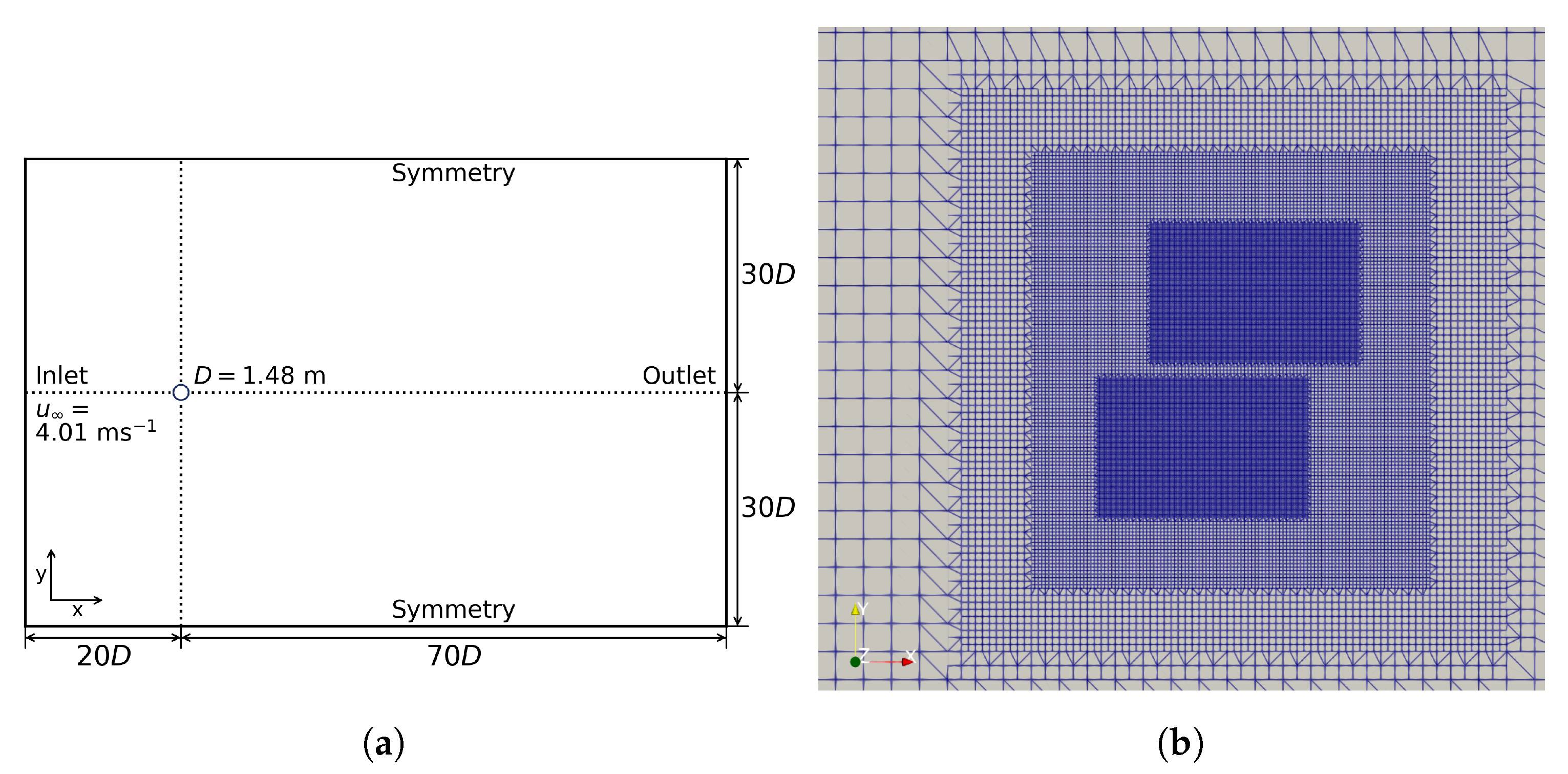
2.2. Turbine Geometry and CFD Setup

The turbine that will be studied in our work is a 2-bladed H-type VAWT, which was measured in the wind tunnel experiments conducted by LeBlanc & Ferreira [48] and used in the ALM investigations reported by Zhao et al. [34]. This turbine was specifically chosen owing to the availability of both experimental data and ALM results, so it lends itself well to a validation of Bachant et al.’s [39] implementation. Table 1 lists the important turbine properties and the operating point for a TSR of λ = 3.7 (for an inflow wind speed of 4.01 m s 1 ). No additional structure (e.g., shaft and/or struts) outside of the blades is included for consistency with the simulations conducted by Zhao et al. [34]. We chose a single, fixed TSR for our simulations in order to focus our investigative efforts on the relationship between the turbine array configuration and the multi-turbine synergy. Furthermore, the value of λ = 3.7 is specifically chosen because it avoids the occurrence of dynamic stall [34], a phenomenon that hinders aerodynamic efficiency [26]. Therefore, dynamic stall correction and other add-on models provided by Bachant et al. [39] can be disabled to allow for a direct comparison with Zhao et al.’s [34] results (which did not employ such models), while still ensuring appropriate simulation accuracy. The airfoil data table used for all the ALM calculations in this study is the R e c = 10 6 dataset for the NACA 0021 airfoil retrieved from Sheldahl & Klimas [47], which is consistent with that used by Zhao et al. [34].
Table 2 displays the CFD parameters for all ALM simulation cases conducted using the turbinesFoam library. These parameters are identical to Zhao et al.’s [34] setup with the exception of an enlarged domain, which, in terms of the rotor diameter, is about 91.2 D × 60.8 D × 1.9 D . This is in accordance with the guidelines set out by Balduzzi et al. [49] and followed by Bachant et al. [39]: namely, to use a domain size of at least W = 60 D × L = 90 D in order to ensure that the boundaries of the computational domain are consistent with an open field and mitigate blockage effects (which are found to inflate ALM forces).
Figure 2 illustrates the domain and mesh for the current ALM simulations. Note that all CFD cases are 3-D URANS with the k- ω SST turbulence model, which was chosen to ensure consistency with Zhao et al.’s [34] setup and direct comparability of ALM results. We retain the boundary conditions used by Bachant et al. [39,44]. In each case, the isolated turbine or groups of turbines will be centered at a location 20D downstream of the inlet plane, which efficiently utilizes the domain space and consistently minimizes the impact of the lateral boundaries on the ALM results. A step-wise mesh refinement process is used to set the cell size in the vicinity of the virtual VAWTs. More specifically, in snappyHexMesh, two refinement regions followed by an additional region per turbine are used to refine the mesh procedurally from level 2 to level 4. The background mesh is defined such that the level 4 mesh (innermost cells of the mesh) has a size of about 0.05 m in each direction (consistent with Zhao et al. [34]), which covers a region of W = 4 m × L = 6 m . Note that the boundary-layer mesh near the blade surfaces is not required, since the presence of the blades is modelled virtually in ALM. The next two levels are defined over conjoined refinement regions encompassing all turbines, with lengths and widths based on the maximum dimensions of the inner region and the inclusion of two meters of padding on each side. The coarse global mesh has a cell size of about 0.8 m. It is challenging and expensive to systematically verify the mesh size in an ALM simulation, since the physics being emulated are sensitive to the combination of the cell size and the Gaussian kernel width ϵ . These two parameters must be investigated in conjunction, since different Gaussian widths require different spatial and temporal CFD resolutions [34]. Therefore, a separate grid-independence study was not performed in this case, and, instead, we follow Zhao et al.’s [34] mesh settings for the 2-bladed VAWT being investigated herein.

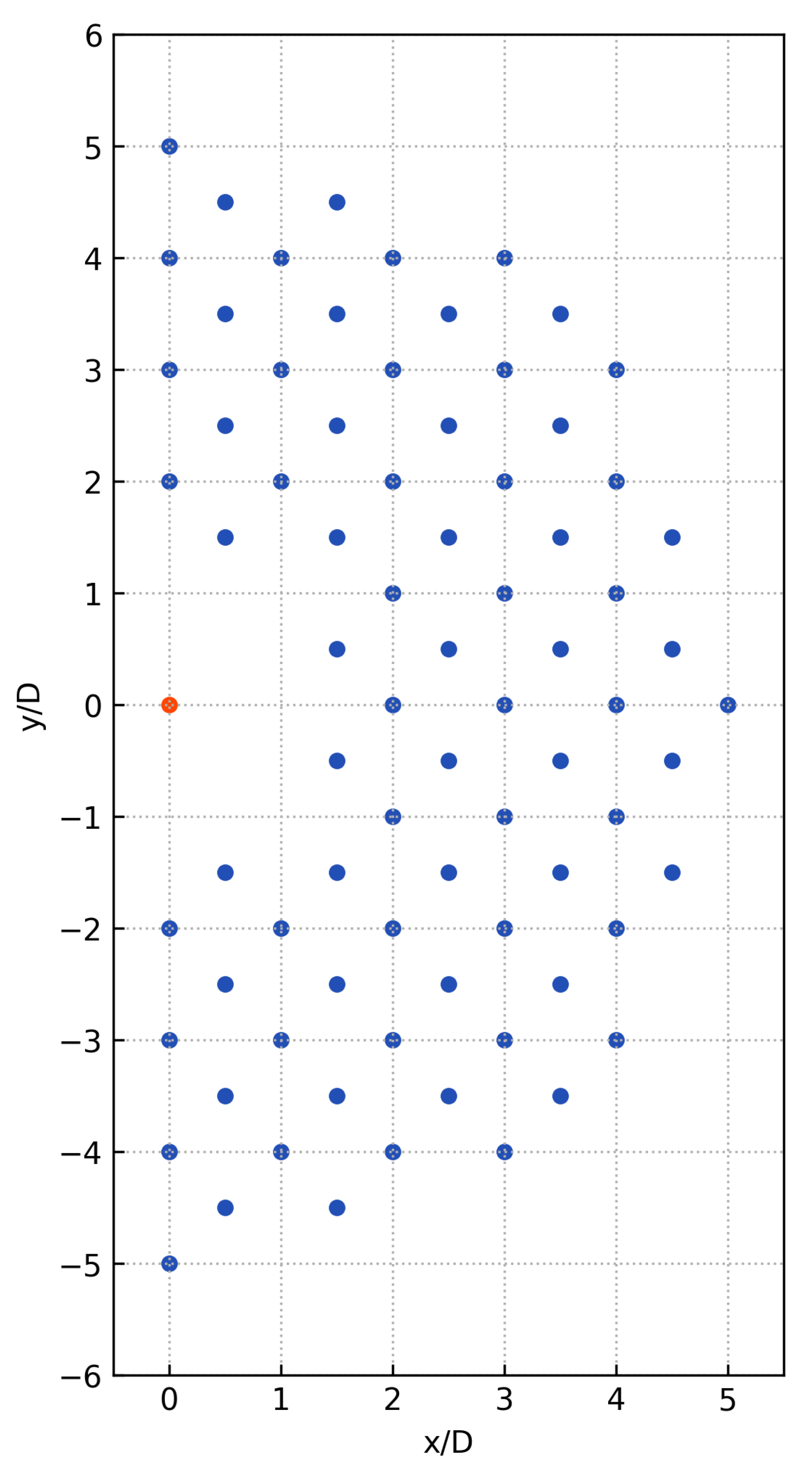
2.3. Two-Turbine Group (Array) Configurations

The design of the configurations of the two-turbine groups that will be simulated using ALM is vital. Previous literature loosely explored the configuration space, with Hansen et al. [23] being the only study to systematically test two-turbine cases. Hansen et al. labels the two turbines as rotor 1 (R1) and rotor 2 (R2) and parameterizes R2’s relative position to R1 using an array angle β and a turbine spacing d i s t . For some fixed d i s t = 1.375 D , 2 D , and 3 D , the normalized power-generation performance of R1 and R2 can be plotted as a function of β in the range [ 90 , 90 ] , where a magnitude of 90 corresponds to the adjacent arrangement for which the turbines are side-by-side facing the incident wind direction. Hansen et al. [23] claimed that “this is the first attempt at numerically investigating the efficiency augmentations of VAWTs for more than 20 different layouts” [23]. This is a landmark achievement for optimizing VAWT layouts through the consideration of the unique synergistic phenomenon, and we seek to expand (extend) considerably these results using a reduced-order model based on ALM simulations, rather than a full-order model based on blade-resolved CFD simulations.
Figure 3 illustrates the suite of wind-turbine-array layouts that will be simulated using ALM. For ease of reference, we label the turbines T1 and T2, where T1 is the leading (or, upwind) turbine in non-adjacent (side-by-side) arrangements. Due to the fact that only the relative positions matter in the layout, we fix T1 at ( 0 , 0 ) (origin of the Cartesian coordinate system) and vary T2’s position in a staggered grid around T1 at a downwind x-spacing of 0.5D and a crosswind y-spacing of 1D. Figure 3 resembles half of a donut shape, because the left half of the configuration space (where T2 would be the leading or upwind turbine) is eliminated owing to symmetry. The “hole” surrounding T1 is present in order to avoid simulating pairwise interactions where the spatial proximity of the two turbines is so close that there is no reliable way to ascertain the validity of ALM. For instance, ALM is unable to capture the collision of blades when the turbines overlap. An upper limit is also set to allow for a feasible yet useful configuration space, enabling the meaningful evaluation of synergy up until the separation distance sufficiently weakens such interaction effects. We will simulate all 78 of the shown two-turbine layouts with co-rotating turbines (viz. with the blades of both turbines rotating CCW), as well as a reduced grid size of 30 counter-rotating cases (viz. with T1 rotating CCW and T2 rotating clockwise or CW), forming a total of 108 two-turbine cases that will be simulated. To our knowledge, this is the largest number of cases simulated to date, using either full-order modeling based on a blade-resolved CFD or reduced-order modeling based on ALM.

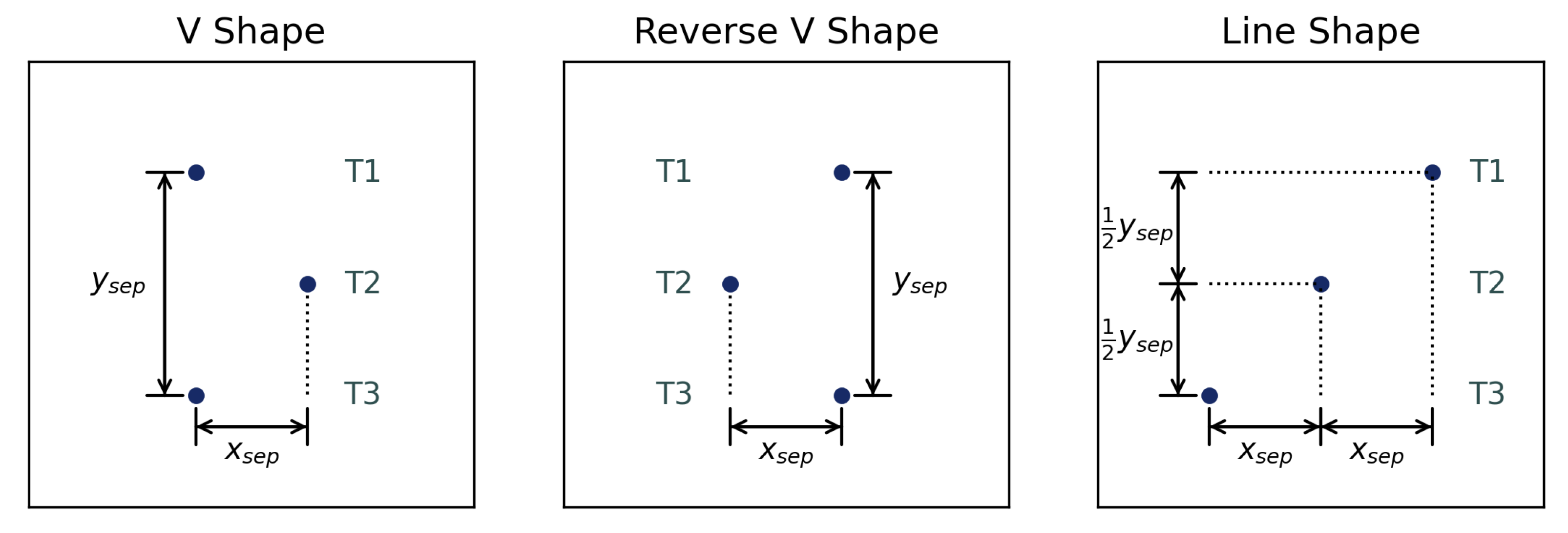
2.4. Three-Turbine Group (Array) Configurations

It is more difficult to parameterize the three-turbine configurations in a comprehensive manner due to the additional degree of freedom. Therefore, based upon the synergy patterns derived from the two-turbine results, three promising shapes are used within the three-turbine groupings—it is expected that these designs will manifest a net cluster-level synergy. In Figure 4, with an incident wind direction from left to right, the V, Reverse V, and Line shapes (configurations) are defined. All turbines will be co-rotating with respect to each other in the CCW direction. The definition of the spacing parameters x s e p (in the downwind direction) and y s e p (in the crosswind direction) is consistent across the three array configurations, with x s e p = ( 0.34 D , 0.50 D , 0.68 D ) for the V and for the Reverse V configurations and x s e p = ( 0 , 0.34 D , 0.50 D , 0.68 D ) for the Line configuration. Finally, y s e p = ( 3 D , 4 D , 5 D , 6 D ) for all these three-turbine array configurations. These constitute a total of 40 ALM cases for the three-turbine groups.

2.5. Synergy Superposition Scheme

A novel proposition in this study is the idea of a “synergy superposition scheme”. Inspired by the synergy patterns which will be discussed in the next section, we formulated the hypothesis that three-turbine cluster synergy may be approximated as a linear superposition of all the possible pairwise VAWT interactions contained therein. The specific procedure to test this hypothesis involves identifying every relative pairwise sub-arrangement in each of the 40 three-turbine configurations and simulating those ALM cases. Following on from this analysis, the superposed estimate of some turbine’s power ratio is formulated as follows.
C P C P , i s o s = 1 + i = 1 n C P C P , i s o i 1 ,
where the subscript s denotes the superposed (approximate) power ratio of some turbine in the three-turbine group, and the summation is computed for n = n t 2 pairs indexed as i (here, n t is the number of turbines in the array so, for example, n = 3 2 = 3 for a three-turbine cluster). The power coefficient C P of the i-th turbine depends on the turbines in each pair that correspond to the same relative positioning in the greater cluster. Essentially, this assumes that the deviation of the power ratio from 1 is a quantity that can be linearly superposed via summation. This scheme is a simple one, and the formulation is arbitrarily chosen to serve as a starting point towards demonstrating a proof-of-concept.

3. Results and Discussion
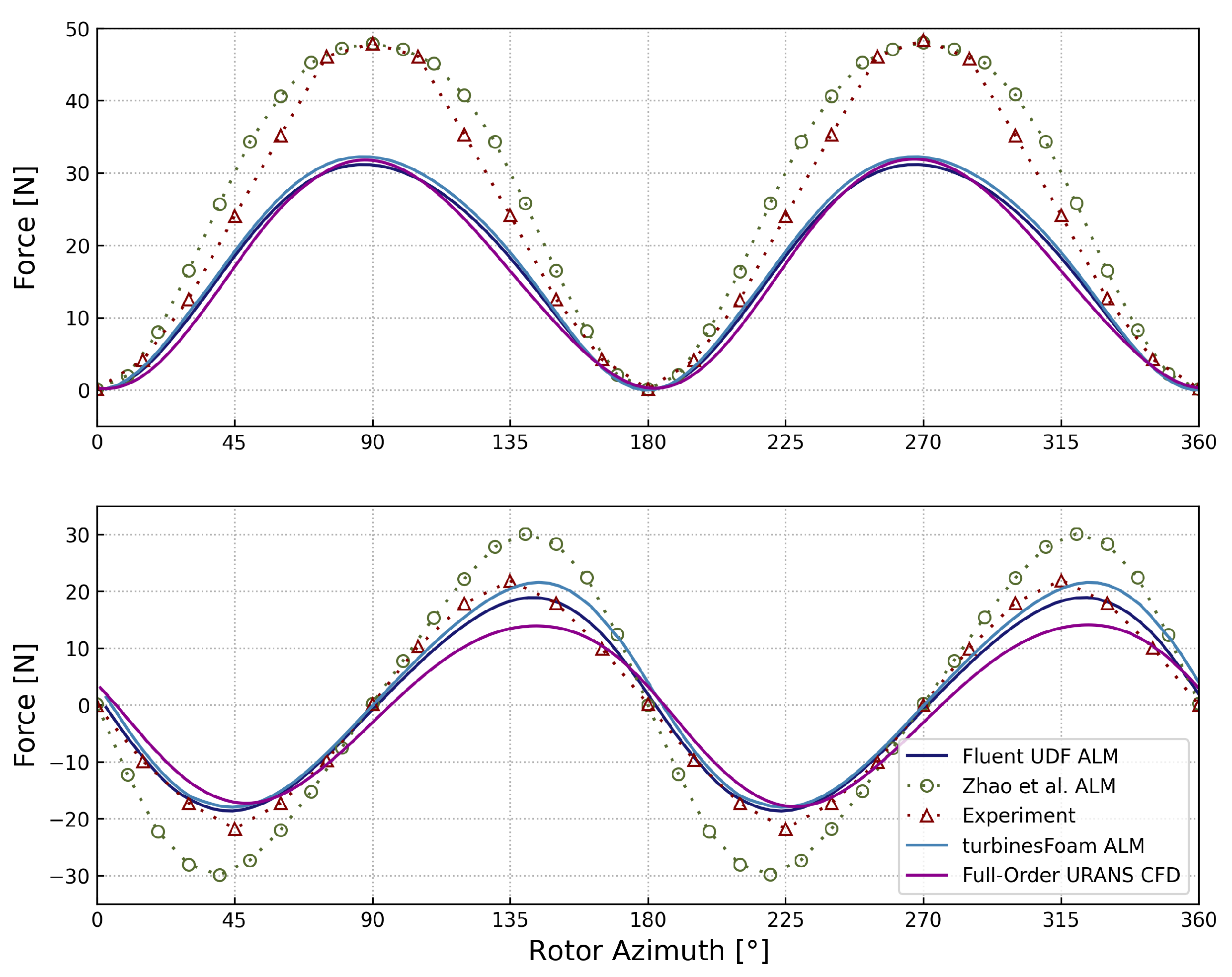
3.1. Validation

We now present a validation of the currently used turbinesFoam ALM library for the isolated VAWT being studied. The first simulation result in Figure 5 is obtained using a separate ALM code we developed for Fluent using the User-Defined Functions (UDF) framework. This implementation is entirely based on an interpretation of Zhao et al.’s [34] approach, which used a 2-D Gaussian kernel for force projection and smoothing. For comparison, Zhao et al.’s [34] ALM results, the experimental measurements obtained by Leblanc & Ferreira [48], and the ALM simulation results obtained using Bachant’s [39] OpenFOAM code (turbinesFoam) are displayed. Finally, the last result used in the comparison is a 2-D full-order blade-resolved CFD simulation (URANS with the k- ω SST turbulence model) of the same 2-bladed turbine. This case was generated and conducted in ANSYS Fluent 2020 R2 with a steady-state initialization run (using a Moving Reference Frame) followed by a transient run (using a Sliding Mesh procedure), closely following a similar CFD case undertaken by Abdalrahman [11]. Each of the two blades is meshed with 600 cell divisions around the profile and 50 layers of inflation cells, beginning at a first layer with a thickness of 1.08 × 10 5 m, guaranteeing that the non-dimensional wall-normal distance y + is less than five throughout the simulation. All other setup parameters are consistent with those shown in Table 2, consequently, conform with what has been documented by Zhao et al. [34].
A comparison of the results in Figure 5 shows that the general trends of the turbine force components F x and F y in the x- and y-directions, respectively, to concur generally across all the simulation and experimental measurements, although some discrepancies in magnitude exist (especially near the peaks). The values for F x obtained from the ALM simulations conducted by Zhao et al. [34] and from the experimental measurements of Leblanc & Ferreira [48] are most notably underpredicted by the current turbinesFoam ALM simulations, the Fluent UDF ALM simulations, and the full-order URANS CFD simulations, although these three simulations results conform very well with one another. It is worth noting that, between the two ALM simulations, the cases are standardized in terms of mesh, Gaussian width ( ϵ ), and airfoil data ( R e c = 10 6 from Sheldahl & Klimas [47] in accordance with the setup of Zhao et al. [34]). However, for the values of F y , the results from these three simulations are in excellent conformance with experimental measurements, whereas those of Zhao et al. [34] over-predict the transverse ( F y ) forces.
There may be several reasons for the mis-prediction of the current ALM results. Firstly, the airfoil data is synthesized and not experimentally obtained [39], and the static airfoil data would likely be unable to fully represent the loading on dynamically pitching airfoils, as is the operational reality for the VAWT blades. Mendoza & Goude [46] also demonstrated a tendency for these airfoil data tables to under-predict the turbine blade forces when compared to the lift and drag coefficients generated by the XFOIL program. Scheurich & Brown’s [50] study found that using only static airfoil data led to significant under-predictions of the sectional tangential force coefficient near the extremes in the range of the angle of attack (viz., | α | 15 ), whereas a dynamic stall model was able to produce large aerodynamic force coefficients. This points to some uncertainty as to whether a value of TSR of λ = 3.7 is truly sufficient to avoid dynamic stall. Abhishek [3] also found that a lack of correction for virtual camber, which arises in symmetrical airfoils operating in a curvilinear flow (blade rotation), can account for an under-prediction of C l by 0.4–0.65. Finally, a similar magnitude of under-prediction can be found in Bachant et al.’s [39] validation for the RM2 turbine. In view of this, we hereby proceed with the current approach, since the two ALM simulation results are in good conformance with the full-order blade-resolved CFD simulations results, and the mis-predictions are within reasonable limits. Finally, it is noted that synergy is a relative measure of performance normalized by C P , i s o , so the accurate prediction of the absolute value of C P may not be as critical.

3.2. Two-Turbine Group (Array) Results

Using the current ALM methodology, the isolated turbine-power coefficient C P is determined to be 0.5458 . We find that the stream-wise velocities are enhanced or sped-up in a region adjacent to the rotor and surrounding the wake, implying that u / U 0 > 1 (where u is the stream-wise velocity component, and U 0 is the freestream (incident) velocity). A sample of the flow field illustrating this velocity speed-up effect is presented in Figure 6. This is consistent with the previous findings of Zanforlin & Nishino [17], Lam & Peng [18], Brownstein et al. [22], and Hansen et al. [23]. Using this baseline C P , i s o , the heatmaps in Figure 7 (showing T1 and T2 power ratios) and Figure 8 (showing the cluster mean power ratio) can be obtained, which include the 78 array layouts for the pairwise co-rotating turbines.
There are three sets of data to present for the two-turbine cases, namely, T1, T2, and the cluster mean power ratios (sum of C P of both turbines divided by 2 C P , i s o ). Each set is visualized in its own heatmap, where T1 is fixed at the coordinates ( 0 , 0 ) and a coordinate of ( x / D , y / D ) indicates a layout with T2 located there (similar to Figure 3). Each diamond-shaped cell’s color-coded power ratio value is defined by the layout, which contains T2 located at that cell’s center. This provides a convenient overview of the synergy landscape for a pair of turbines when the T2 position is parameterized in a staggered grid fashion. Between the heatmaps presented in Figure 7 and Figure 8, it is clear that a wide range of layouts is indeed capable of generating synergy (viz., cells are colored green), as predicted by the ALM simulations. This serves to demonstrate that there appear to be no fundamental barriers which may inhibit the ALM simulations from expressing VAWT synergy.
Additionally, we may also extract some useful synergy patterns from a careful perusal of these plots. In Figure 7a, T1 (the leading or upwind turbine in non-adjacent layouts) benefits the most from synergy when T2 is adjacent to T1 (i.e., they are in the same column) or slightly downstream from those configurations. Notice the broad patterns are mirrored across the x-axis, but there are subtle asymmetries, which are likely due to the inherent wake asymmetry unique to VAWTs. The power performance of T1 also diminishes not only when T2 lies directly within T1’s wake ( y / D in the range [ 0.5 , 0.5 ] ), but also in a sector of approximately 90 or more. This provides evidence of a blockage effect, which occurs when a downwind turbine (T2) blocks the flow through the upwind turbine, decreasing its power-generation performance. This blockage effect is well-documented in the works of Zanforlin & Nishino [17], Shaaban et al. [20], Brownstein et al. [22], and Hansen et al. [23]. Using the heatmap visualization of T1, it is possible to observe the gradual transition from a power detriment (due to blockage) to a synergistic interaction across the configuration space.
Simultaneously, the effects of these layout changes on T2 (the downwind turbine) can be ascertained from a careful examination of Figure 7b. Interestingly, T2 experiences synergy almost universally, with the only (predictable) exception being the cases where T2 is situated in the velocity-deficit region of T1’s wake. Another useful observation is that T2 generally experiences greater synergy—about 2% more than T1 in terms of the most favorable synergistic arrangements. The most favorable synergistic cases for T2 also deviate from T1’s preference for adjacent configurations and are instead located along a band just outside of the wake region (at | y | / D = 1.5 ) and at some distance downstream of T1 ( x / D 0.5 ). In fact, this correlates with the high-velocity flow acceleration regions found adjacent to the turbine wake, which is a phenomenon also observed by Hansen et al. [23]. Moreover, further evidence for an accelerated fluid flow [51] around two rotating VAWTS arranged side-by-side (yielding increased power generation or synergy) has been provided using flow visualization [52] and CFD simulations to study the dynamic fluid-body interaction [53]. While we do not claim to contribute to the fundamental understanding of the physics that drive synergy, it is conceivable that higher ALM forces can be produced when the stream-wise velocity is augmented, since the force is a function of the magnitude of u r e l .
Finally, the cluster mean power ratio heatmap in Figure 8 is useful for assessing the synergistic potential of the entire two-turbine group. Due to the generally larger synergy magnitudes of T2, cluster mean patterns are expectedly similar—almost all the layouts are advantageous over the isolated, baseline case. However, the competition effect remains crucial in determining the optimal configuration, which is a compromise between the adjacent arrangements (favored by T1) and downstream arrangements (favored by T2). The optimal synergy is found at a T2 oriented at 71 . 6 and spaced at 1.58 D relative to T1, which produces a cluster-level power ratio of 1.0247. This means the cluster would produce 2.47% more power compared to two individually operating (isolated) turbines. The synergy patterns presented herein agree well with Hansen et al.’s results, namely, a maximum in T1 synergy in the adjacent configurations, an asymmetric bias of synergy in favor of the bottom-half of the layouts (T2 below T1), and T1’s power-generation performance decrease due to the proximity of T2 to T1’s wake [23]. This overall consistency lends credence to our methodology, and these results offer a unique perspective on the relationship between turbine layout and synergy, which complements and elaborates upon previous investigations.
The 30 counter-rotating cases are presented in Figure 9 and Figure 10. These exhibit essentially the same macro-patterns with small differences in the synergy magnitudes for some layouts, possibly attributable to the opposite blade-rotation scenarios. This is also consistent with Hansen et al.’s [23] results. We find the optimal configuration in the counter-rotating case to be identical to the co-rotating case ( 71 . 6 angle and 1.58 D spacing between T1 and T2), but the power ratio is 1.0266, which is slightly larger than the co-rotating case. Overall, across all configurations, neither the co-rotating nor the counter-rotating cases dominate in cluster-level synergy—in fact, the favorable cases are evenly split with a less than 1% difference. This indicates there is no practical preference for co-rotating or counter-rotating arrays after considering the likely variations of the incoming wind direction.

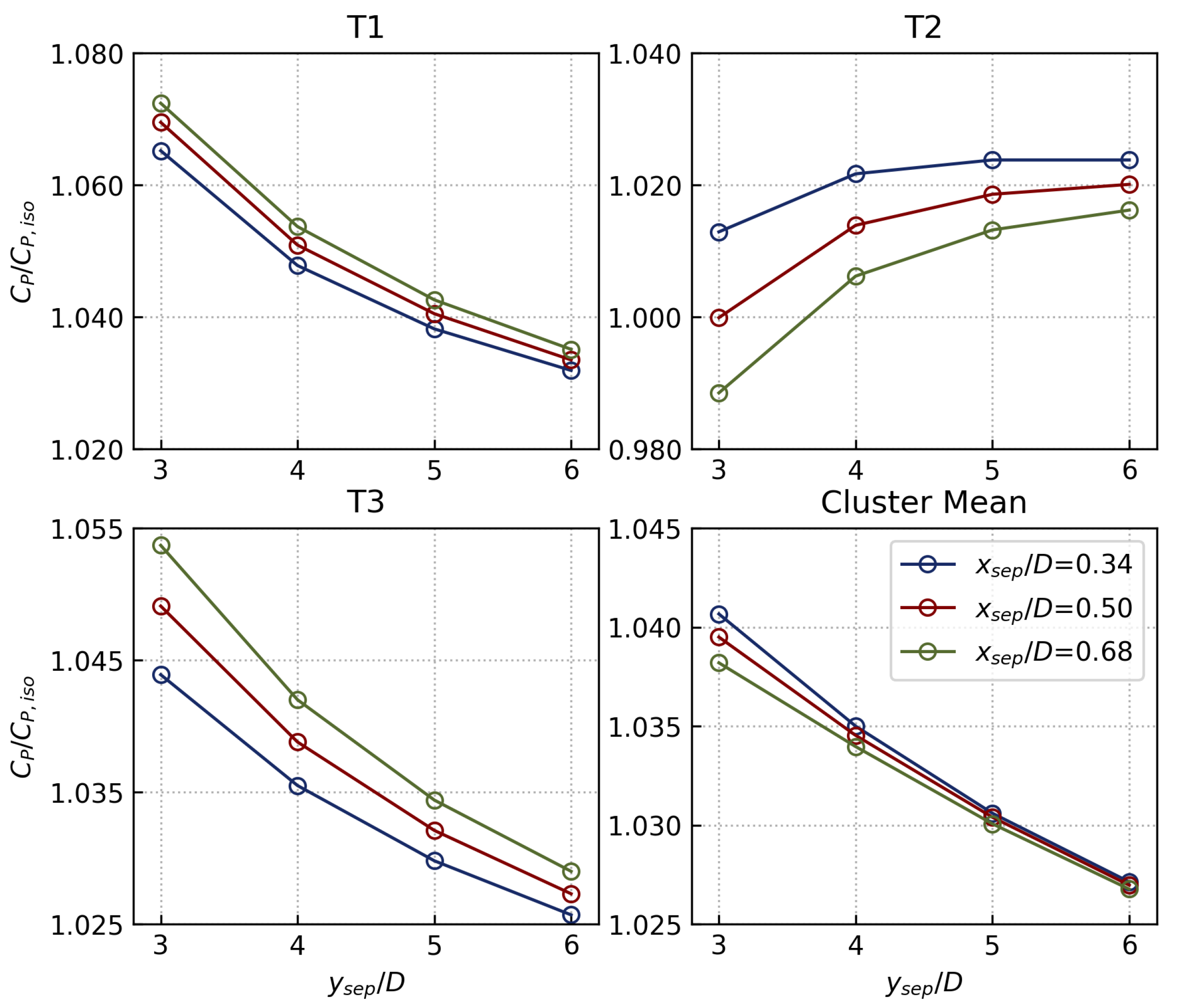
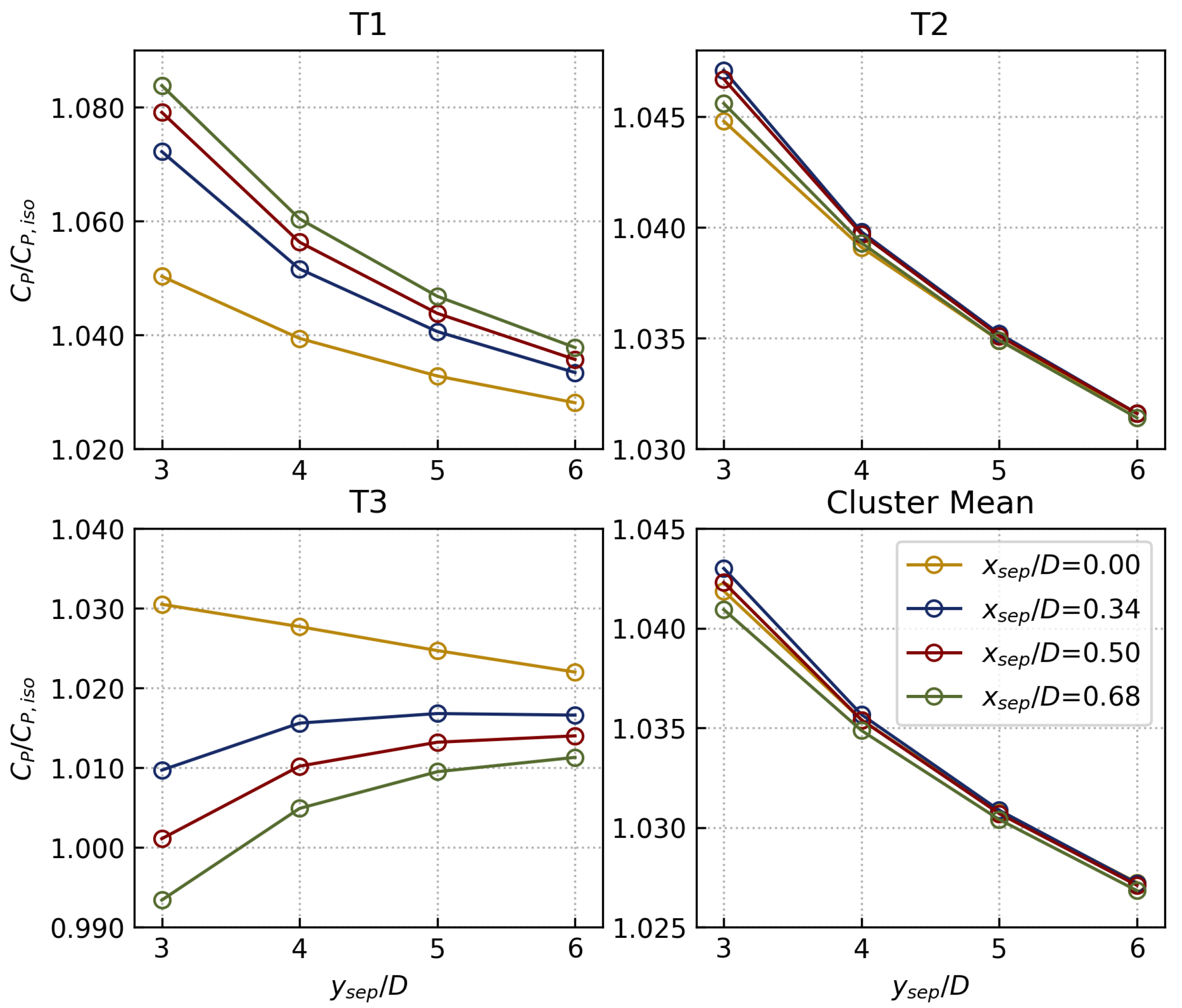
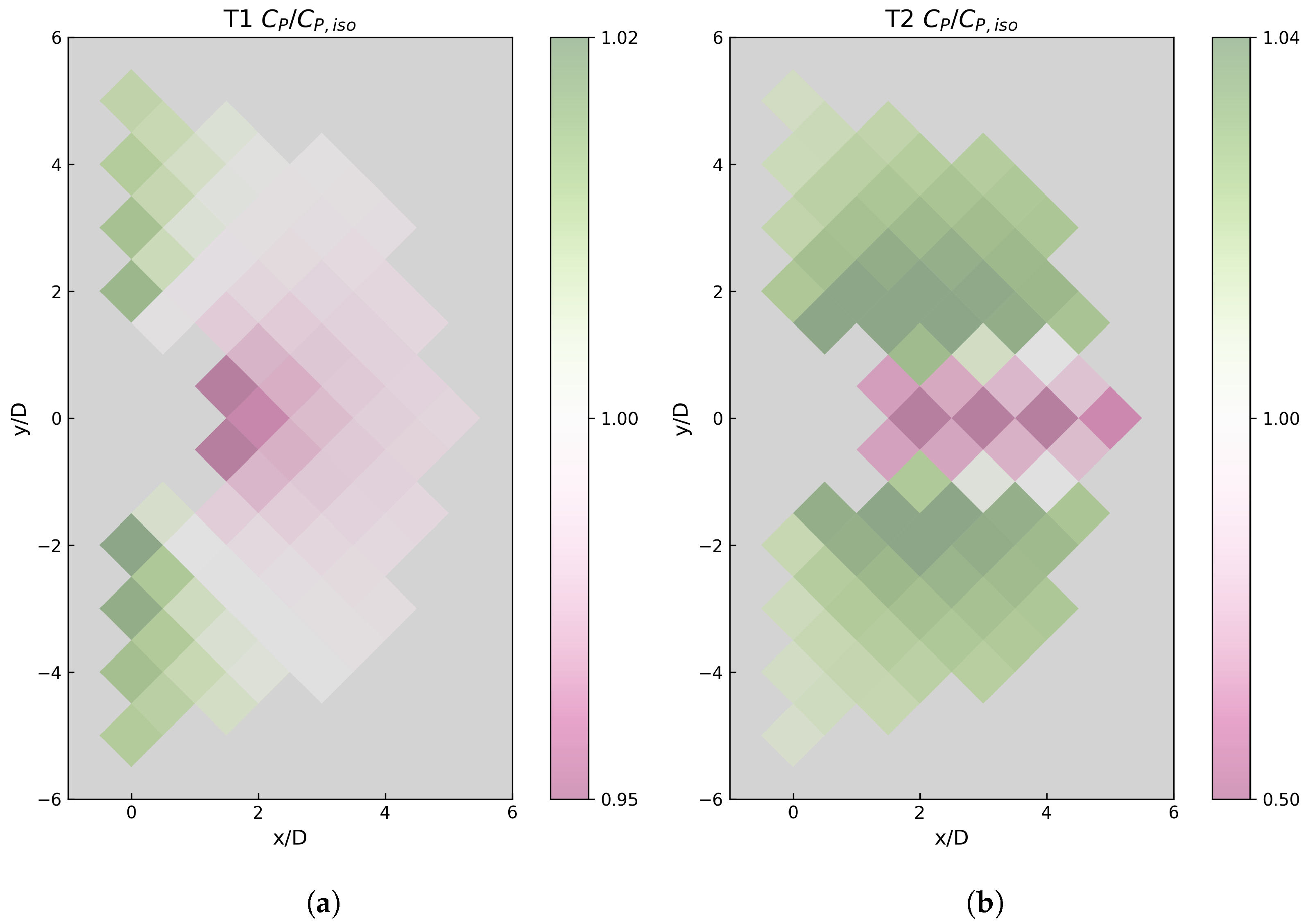
3.3. Three-Turbine Group (Array) Results

For the three-turbine group results, the power ratios as a function of the spacing parameters ( x s e p and y s e p ) are plotted in Figure 11 (V), Figure 12 (Reverse V), and Figure 13 (Line). The power ratios of T1, T2, T3, and the cluster are divided into the respective subplots in each figure. We are able to identify general synergy patterns that hold across all cases despite the differences in the array layout shapes. Specifically, the leading (upwind) and trailing (downwind) turbines share common functional relationships with the spacing parameters. Referring to Figure 4, T1 and T3 are the leading turbines in the V shape, T2 is leading turbine in the Reverse V shape, and T3 is leading turbine in the Line shape. Similarly, T2 is the trailing turbine in the V shape, T1 and T3 are trailing turbines in the Reverse V shape, and T1 is trailing turbine in the Line shape. It is important to note that T2 is an “intermediate” turbine, which is positioned between the most upwind and downwind turbines, and the implications of this will be discussed shortly.
In fact, the two-turbine group synergy patterns are useful even in the context of the interpretations of the characteristic synergy patterns apparent in three-turbine groups. For example, with regard to the trailing turbines, the functional relationships between the subplots are qualitatively similar. There is a consistent decrease of the power ratio with an increase in the crosswind separation y s e p , corresponding to an intensification of synergy in the | y | / D = 1.5 bands of Figure 7b and Figure 9b. Again, a plausible reason for this is that the downwind turbine is exploiting the accelerated flow ( u / U 0 > 1 ) that is most pronounced in this region. As the downwind separation x s e p increases, the power ratio also increases. While it may seem counter-intuitive, this is essentially reflecting the pattern that the optimal downwind turbine placement is not at the adjacent location ( x s e p = 0 ), but rather increases with x s e p until some maximum before decreasing. The currently investigated range has an upper bound of x s e p = 0.68 D , which is not sufficiently far downstream to reveal this convex variation with increasing downstream separation of the turbines.
The situation for the leading turbines can be explained in a similar manner. To begin, the power ratio decreases with x s e p consistently, matching the pattern seen in Figure 7a and Figure 9a. When T2 begins to move downwind of T1, the synergistic benefit for T1 weakens, and the detrimental dynamic of the blockage effect strengthens, both resulting in the deterioration of the power-generation performance of T1. In terms of y s e p , the patterns also vary with x s e p and can change from a straightforward, strictly decreasing pattern (e.g., x s e p / D = 0.34 in the T1 subplot of Figure 11) to a convex (parabolic) variation that exhibits a maximum value (e.g., for x s e p / D 0.50 in the same subplot). There appears to be a strong connection between this functional relationship and the presence of a contest between the synergistic effect and the negative blockage effect, both due to the interaction with a downwind T2. For the intermediate turbine (T2 in Figure 13), the aforementioned dynamics of the leading and trailing turbines are both in play, creating competition. The competing dynamics are evidenced in the compactness of the variation of the data points, both in terms of x s e p and y s e p . We see that, as a consequence, the most favorable x s e p distance for power production does not follow a strictly monotonic ascending or descending pattern (viz., x s e p = 0.34 D has the largest power ratio, followed by 0.5 D , 0.68 D , and then, disruptively. 0, for y s e p = 3 D ). In fact, this contention parallels the trend in the cluster mean of all three array configurations, wherein the synergy patterns are “averages” of the individual leading and trailing turbine dynamics that constitute the cluster.
Overall, the three-turbine group cases simulated herein demonstrate their general feasibility as successful synergy-producing configurations. There are limitations to studying the power ratio as a function of the x and y spatial configuration parameters, since the underlying synergistic principles do not necessarily conform to this framework. For instance, T1’s synergy patterns are better contextualized with angle and spacing parameters (as performed by Hansen et al. [23]), but the correlation of T2 synergy to a high-velocity band surrounding the wake can be more saliently recognized when the layouts are organized on a Cartesian grid. Additionally, heatmaps do not extend well to three-turbine cases, where the larger number of degrees of freedom obscures efforts for a holistic visualization. Despite this, valuable insight has been generated, and these can provide useful design heuristics if not rules in VAWT wind-farm micro-siting. For example, the cluster mean power ratios in the V and Reverse V turbine groupings are nearly identical (with no practical difference in value). While this is not entirely surprising, because these shapes are mirrored across the y-axis with respect to each other, this result seems to suggest that there may be a “conservation” of synergy. In other words, inserting additional downwind turbines to exploit the flow-field of an upwind turbine would proportionally diminish the overall synergy due to blockage. This is an interesting idea that warrants further investigation.

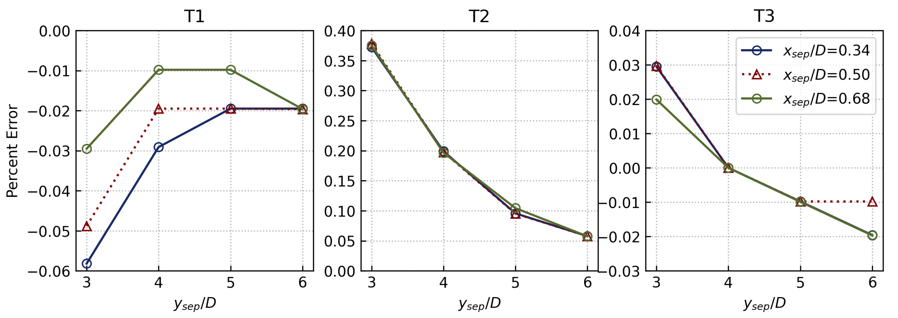
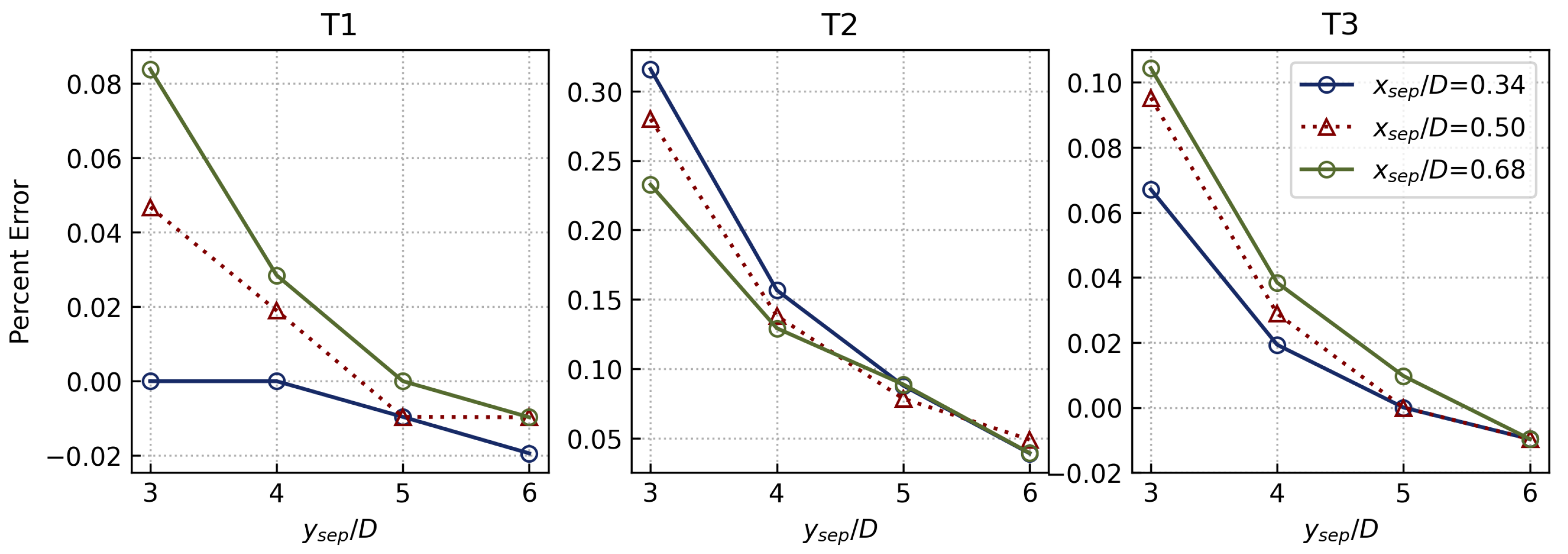
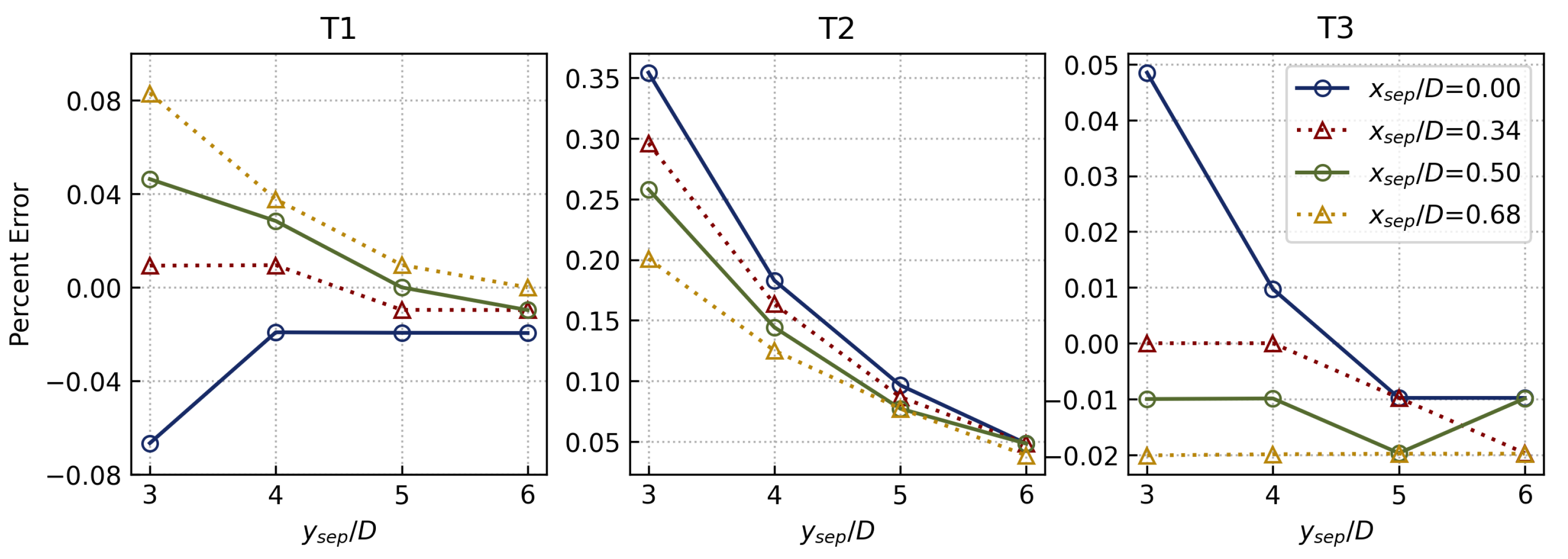
3.4. Synergy-Superposition Scheme Results

Here we present the results of the synergy-superposition scheme, which is an entirely novel idea (to the best of our knowledge). Using the scheme and procedure detailed above, the approximate power ratios are calculated and compared to the complete three-turbine ALM simulation results. The percent differences are displayed in Figure 14, Figure 15 and Figure 16 for the V, Reverse V, and Line turbine groupings, respectively. Overall, the error magnitudes are bounded within 0.38%, 0.32%, and 0.35% for the V, Reverse V, and Line shapes, respectively. This is a remarkably close agreement, demonstrating the validity of the superposition scheme within the scope of this work. It is important to caution the reader that the error plots exhibited here may not contain meaningful information or patterns beyond the noise associated with the numerical (round-off) errors expected of the simulations. Furthermore, while this scheme appears promising, its generalizability remains to be determined using larger turbine groups and especially using full-order blade-resolved CFD simulations for validation. Perhaps the first-order, linear effects superposed here are adequate for predicting three-turbine group synergistic interactions (for the current turbine and operating conditions), but larger errors may arise in extending this to an N-turbine group ( N 4 ) due to the emergence of elusive higher-order dynamical interactions.

4. Conclusions

In this work, we have presented a methodology for using an ALM code (turbinesFoam) to evaluate synergy in VAWT groups consisting of two and three turbines. The code has been validated and used in previous investigations, and a comparison has been performed with 2 other ALM simulations codes, with a 2-D full-order blade-resolved URANS CFD simulation, and with available experimental measurements. A key result obtained herein was the successful demonstration that ALM simulations are capable of predicting VAWT synergy, yielding generally very good conformance to the pairwise turbine synergy patterns documented in the previous literature. Furthermore, we used a total of 108 two-turbine and 40 three-turbine ALM simulations to map the variation of turbine power-generation performance (characterized using a power ratio) arising from the systematic variation in the turbine array layout parameters. We find that a downwind turbine benefits almost universally from operating in the proximity of an upwind turbine (except in the wake regions), while the upwind turbine’s synergy is equalized or diminished due to the blockage from this downwind turbine. It is also shown that co- and counter-rotating pairs are both capable of generating synergy, and neither offers an appreciable (significant) advantage over the other. Within the currently used methodology, it is possible to identify an optimal two-turbine layout that maximizes the cluster-level synergy. This pattern generalizes well to three-turbine cases and contributes value by explaining three-turbine synergistic interactions in a more granular way. We push the envelope further by proving the effectiveness and accuracy of a novel synergy-superposition scheme, confirming that a three-turbine group’s synergy can be adequately modeled as a linear superposition of all the pairwise interactions in the three-turbine array.
These results could be enhanced by future work in the following ways. First, the isolated turbine performance could be more rigorously validated. This may be achieved by obtaining a high-fidelity airfoil coefficient dataset (possibly driven by full-order URANS CFD simulations), exploring various additional correction models (e.g., for dynamic stall), and testing different Gaussian kernel formulations. It is recommended that multi-turbine full-order blade-resolved CFD simulations be performed to thoroughly and systematically evaluate the accuracy of ALM simulations in predicting VAWT power-generation performance. Furthermore, it would be valuable to extend the present investigation to larger turbine groups (four or more turbines in the array), to more diverse turbine geometries or heterogeneous wind farms, and to different TSRs. The current model is also suitable for extension towards the evaluation of synergy in complex terrain situations, for which a different lower-boundary condition can be imposed to represent the complex terrain. The virtual turbines can also be freely arranged both in the horizontal plane and the vertical direction, using the ALM technique, in order to capture the synergy in sophisticated cases such as an urban siting. The use of a low-cost, effective reduced-order approach such as an ALM simulation is expected to be invaluable to the optimal design of large-scale VAWT farms—involving, as such, the leveraging of the unique opportunities provided by turbine synergistic interactions.

Author Contributions

Conceptualization, J.H.Z., F.-S.L. and E.Y.; methodology, J.H.Z., F.-S.L. and E.Y.; software, J.H.Z.; validation, J.H.Z.; formal analysis, J.H.Z.; investigation, J.H.Z., F.-S.L. and E.Y.; resources, F.-S.L.; data curation, J.H.Z.; writing—original draft preparation, J.H.Z.; writing—review and editing, E.Y. and F.-S.L.; visualization, J.H.Z.; supervision, F.-S.L. and E.Y.; project administration, F.-S.L. and E.Y.; funding acquisition, F.-S.L. All authors have read and agreed to the published version of the manuscript.

Funding

This research was funded by the Natural Sciences and Engineering Research Council of Canada (NSERC) Discovery Grants program Grant No. 50503-10234.

Institutional Review Board Statement

Not applicable.

Informed Consent Statement

Not applicable.

Conflicts of Interest

The authors declare no conflict of interest.

Abbreviations

The following abbreviations are used in this paper:
ALMactuator line model
BEMblade element momentum
CFDcomputational fluid dynamics
HAWThorizontal-axis wind turbine
TSRtip-speed ratio
URANSunsteady Reynolds-Averaged Navier–Stokes
VAWTvertical-axis wind turbine

References

  1. Möllerström, E.; Gipe, P.; Beurskens, J.; Ottermo, F. A historical review of vertical axis wind turbines rated 100 kW and above. Renew. Sustain. Energy Rev. 2019, 105, 1–13. [Google Scholar] [CrossRef]
  2. Liu, K.; Yu, M.; Zhu, W. Enhancing wind energy harvesting performance of vertical axis wind turbines with a new hybrid design: A fluid-structure interaction study. Renew. Energy 2019, 140, 912–927. [Google Scholar] [CrossRef]
  3. Abhishek, P.J.A. Performance prediction and fundamental understanding of small scale vertical axis wind turbine with variable amplitude blade pitching. Renew. Energy 2016, 97, 97–113. [Google Scholar]
  4. Johari, M.K.; Jalil, M.A.A.; Shariff, M.F.M. Comparison of horizontal axis wind turbine (HAWT) and vertical axis wind turbine (VAWT). Int. J. Eng. Technol. 2018, 7, 74–80. [Google Scholar] [CrossRef]
  5. Du, L.; Ingram, G.; Dominy, R.G. A review of H-Darrieus wind turbine aerodynamic research. J. Mech. Eng. Sci. 2019, 233, 23–24. [Google Scholar] [CrossRef]
  6. Ghasemian, M.; Ashrafi, Z.N.; Sedaghat, A. A review on computational fluid dynamic simulation techniques for Darrieus vertical axis wind turbines. Energy Convers. Manag. 2017, 149, 87–100. [Google Scholar] [CrossRef]
  7. Dabiri, J.O. Potential order-of-magnitude enhancement of wind farm power density via counter-rotating vertical-axis wind turbine arrays. J. Renew. Sustain. Energy 2011, 3, 043104. [Google Scholar] [CrossRef]
  8. Paraschivoiu, I. Wind Turbine Design: With Emphasis on Darreius Concept; Presses Internationales Polytechniques: Montreal, QC, Canada, 2009. [Google Scholar]
  9. Nobile, R.; Vahdati, M.; Barlow, J.F.; Mewburn-Crook, A. Unsteady flow simulation of a vertical axis augmented wind turbine: A two-dimensional study. J. Wind. Eng. Ind. Aerodyn. 2014, 125, 168–179. [Google Scholar] [CrossRef]
  10. Elkhoury, M.; Kiwata, T.; Aoun, E. Experimental and numerical investigation of a three-dimensional vertical-axis wind turbine with variable-pitch. J. Wind. Eng. Ind. Aerodyn. 2015, 139, 111–123. [Google Scholar] [CrossRef]
  11. Abdalrahman, G. Pitch Angle Control for a Small-Scale Darrieus Vertical Axis Wind Turbine with Straight Blades (H-Type VAWT). Ph.D. Thesis, University of Waterloo, Waterloo, ON, Canada, 2019. [Google Scholar]
  12. Tavernier, D.D.; Ferreira, C.; van Bussel, G. Airfoil optimisation for vertical-axis wind turbines with variable pitch. Wind Energy 2019, 22, 547–562. [Google Scholar] [CrossRef]
  13. Strom, B.; Brunton, S.L.; Polagye, B. Intracycle angular velocity control of cross-flow turbines. Nat. Energy 2017, 2, 17103. [Google Scholar] [CrossRef] [Green Version]
  14. Kinzel, M.; Mulligan, Q.; Dabiri, J.O. Energy exchange in an array of vertical-axis wind turbines. J. Turbul. 2012, 13, N38. [Google Scholar] [CrossRef]
  15. Hezaveh, S.H.; Bou-Zeid, E.; Dabiri, J.O.; Kinzel, M.; Cortina, G.; Martinelli, L. Increasing the power production of vertical-axis wind-turbine farms using synergistic clustering. Bound.-Layer Meteorol. 2018, 169, 275–296. [Google Scholar] [CrossRef]
  16. Ahmadi-Baloutaki, M.; Carriveau, R.; Ting, D.S. A wind tunnel study on the aerodynamic interaction of vertical axis wind turbines in array configurations. Renew. Energy 2016, 96, 904–913. [Google Scholar] [CrossRef]
  17. Zanforlin, S.; Nishino, T. Fluid dynamic mechanisms of enhanced power generation by closely spaced vertical axis wind turbines. Renew. Energy 2016, 99, 1213–1226. [Google Scholar] [CrossRef]
  18. Lam, H.F.; Peng, H.Y. Measurements of the wake characteristics of co- and counter-rotating twin H-rotor vertical axis wind turbines. Energy 2017, 131, 13–26. [Google Scholar] [CrossRef]
  19. Peng, J. Effects of aerodynamic interactions of closely-placed vertical axis wind turbine pairs. Energies 2018, 11, 2842. [Google Scholar] [CrossRef]
  20. Shaaban, S.; Albatal, A.; Mohamed, M.H. Optimization of H-Rotor Darrieus turbines’ mutual interaction in staggered arrangements. Renew. Energy 2018, 125, 87–99. [Google Scholar] [CrossRef]
  21. Barnes, A.; Hughes, B. Determining the impact of VAWT farm configurations on power output. Renew. Energy 2019, 143, 1111–1120. [Google Scholar] [CrossRef]
  22. Brownstein, I.D.; Wei, N.J.; Dabiri, J.O. Aerodynamically interacting vertical axis wind turbines: Performance enhancement and three-dimensional flow. Energies 2019, 12, 2724. [Google Scholar] [CrossRef]
  23. Hansen, J.T.; Mahak, M.; Tzanakis, I. Numerical modelling and optimization of vertical axis wind turbine pairs: A scale up approach. Renew. Energy 2021, 171, 1371–1381. [Google Scholar] [CrossRef]
  24. Hamada, K.; Smith, T.; Durrani, N.; Qin, N.; Howell, R. Unsteady flow simulation and dynamic stall around vertical axis wind turbine blades. In Proceedings of the 46th AIAA Aerospace Sciences Meeting and Exhibit, Reno, Nevada, 7–10 January 2008. [Google Scholar]
  25. Howell, R.; Qin, N.; Edwards, J.; Durrani, N. Wind tunnel and numerical study of a small vertical axis wind turbine. Renew. Energy 2010, 35, 412–422. [Google Scholar] [CrossRef]
  26. Buchner, A.J.; Lohry, M.W.; Martinelli, L.; Soria, J.; Smits, A.J. Dynamic stall in vertical axis wind turbines: Comparing experiments and computations. J. Wind. Eng. Ind. Aerodyn. 2015, 146, 163–171. [Google Scholar] [CrossRef]
  27. Orlandi, A.; Collu, M.; Zanforlin, S.; Shires, A. 3D URANS analysis of a vertical axis wind turbine in skewed flows. J. Wind. Eng. Ind. Aerodyn. 2015, 147, 77–84. [Google Scholar] [CrossRef]
  28. Zuo, W.; Wang, X.; Kang, S. Numerical simulations on the wake effect of H-type vertical axis wind turbines. Energy 2016, 106, 691–700. [Google Scholar] [CrossRef]
  29. Li, C.; Zhu, S.; Xu, Y.; Xiao, Y. 2.5D large eddy simulation of vertical axis wind turbine in consideration of high angle of attack flow. Renew. Energy 2013, 51, 317–330. [Google Scholar] [CrossRef]
  30. Shamsoddin, S.; Porté-Agel, F. Large Eddy Simulation of vertical axis wind turbine wakes. Energies 2014, 7, 890–912. [Google Scholar] [CrossRef]
  31. Sanderse, B.; van der Pijl, S.P.; Koren, B. Review of computational fluid dynamics for wind turbine wake aerodynamics. Wind Energy 2011, 14, 799–819. [Google Scholar] [CrossRef]
  32. Delafin, P.L.; Nishino, T.; Kolios, A.; Wang, L. Comparison of low-order aerodynamic models and RANS CFD for full scale 3D vertical axis wind turbines. Renew. Energy 2017, 109, 564–575. [Google Scholar] [CrossRef]
  33. Ning, A. Actuator cylinder theory for multiple vertical axis wind turbines. Wind. Energy Sci. 2016, 1, 327–340. [Google Scholar] [CrossRef]
  34. Zhao, R.; Creech, A.C.W.; Borthwick, A.G.L.; Venugoal, V.; Nishino, T. Aerodynamic analysis of a two-bladed vertical-axis wind turbine using a coupled unsteady RANS and Actuator Line Model. Energies 2020, 13, 776. [Google Scholar] [CrossRef] [Green Version]
  35. Sørensen, J.N.; Shen, W.Z. Numerical modeling of wind turbine wakes. J. Fluids Eng. 2002, 124, 393–399. [Google Scholar] [CrossRef]
  36. Hezaveh, S.H.; Bou-Zeid, E.; Lohry, M.W.; Martinelli, L. Simulation and wake analysis of a single vertical axis wind turbine. Wind Energy 2017, 20, 713–730. [Google Scholar] [CrossRef]
  37. Creech, A.C.W.; Borthwick, A.G.L.; Ingram, D. Effects of support structures in an LES actuator line model of a tidal turbine with contra-rotating rotors. Energies 2017, 10, 726. [Google Scholar] [CrossRef]
  38. Abkar, M. Impact of subgrid-scale modeling in actuator-line based large-eddy simulation of vertical-axis wind turbine wakes. Atmosphere 2018, 9, 257. [Google Scholar] [CrossRef]
  39. Bachant, P.; Goude, A.; Wosnik, M. Actuator line modeling of vertical-axis turbines. arXiv 2018, arXiv:1605.01449v4. [Google Scholar]
  40. Melani, P.F.; Balduzzi, F.; Bianchini, A. A robust procedure to implement dynamic stall models into actuator line methods for the simulation of vertical-axis wind turbines. J. Eng. Gas Turbines Power 2021, 143, 111008. [Google Scholar] [CrossRef]
  41. Melani, P.F.; Balduzzi, F.; Bianchini, A. Simulating tip effects in vertical-axis wind turbines with the actuator line method. J. Phys. Conf. Ser. 2022, 2265, 032028. [Google Scholar] [CrossRef]
  42. Melani, P.F.; Balduzzi, F.; Ferrara, G.; Bianchini, A. Tailoring the actuator line theory to the simulation of Vertical-Axis Wind Turbines. Energy Convers. Manag. 2021, 243, 114422. [Google Scholar] [CrossRef]
  43. Raj V, S.; Solanki, R.S.; Chalamalla, V.K.; Sinha, S.S. Numerical simulations and analysis of flow past vertical-axis wind turbines employing the actuator line method. In Proceedings of the 26th National and 4th International ISHMT-ASTFE Heat and Mass Transfer Conference, Tamil Nadu, India, 17–20 December 2021. [Google Scholar]
  44. Bachant, P.; Goude, A.; Wosnik, M. turbinesFoam: v0.0.8.Zenodo. 2018. Available online: https://zenodo.org/record/1210366 (accessed on 3 August 2021). [CrossRef]
  45. Mendoza, V.; Bachant, P.; Ferreira, C.; Goude, A. Near-wake flow simulation of a vertical axis turbine using an actuator line model. Wind Energy 2019, 22, 171–188. [Google Scholar] [CrossRef]
  46. Mendoza, V.; Goude, A. Validation of actuator line and vortex models using normal forces measurements of a straight-bladed vertical axis wind turbine. Energies 2020, 13, 511. [Google Scholar] [CrossRef] [Green Version]
  47. Sheldahl, R.E.; Klimas, P.C. Aerodynamic Characteristics of Seven Symmetrical Airfoil Sections through 180-Degree Angle of Attack for Use in Aerodynamic Analysis of Vertical Axis Wind Turbines; Technical Report SAND8O-2114; Sandia National Laboratories: Albuquerque, NM, USA, 1981. [Google Scholar]
  48. LeBlanc, B.P.; Ferreira, C.S. Experimental determination of thrust loading of a 2-bladed vertical axis wind turbine. J. Phys. Conf. Ser. 2018, 1037, 022043. [Google Scholar] [CrossRef]
  49. Balduzzi, F.; Bianchini, A.; Maleci, R.; Ferrara, G.; Ferrari, L. Critical issues in the CFD simulation of Darrieus wind turbines. Renew. Energy 2016, 85, 419–435. [Google Scholar] [CrossRef]
  50. Scheurich, F.; Brown, R.E. Effect of dynamic stall on the aerodynamics of vertical-axis wind turbines. AIAA J. 2011, 49, 2511–2521. [Google Scholar] [CrossRef]
  51. Zheng, H.D.; Zheng, X.Y.; Zhao, S.X. Arrangement of clustered straight-bladed wind turbines. Energy 2020, 200, 117563. [Google Scholar] [CrossRef]
  52. Jodai, Y.; Hara, Y. Wind tunnel experiments on interaction between two closely spaced vertical-axis wind turbines in side-by-side arrangement. Energies 2021, 14, 7874. [Google Scholar] [CrossRef]
  53. Hara, Y.; Jodai, Y.; Okinaga, T.; Furukawa, M. Numerical analysis of the dynamic interaction between two closely spaced vertical-axis wind turbines. Energies 2021, 14, 2286. [Google Scholar] [CrossRef]
Figure 1. Diagram of a VAWT blade in operation illustrating the ALM formulation, where flow velocities and forces are located at the quarter-chord location ( c / 4 ).
Energies 15 06211 g001
Figure 2. (a) Diagram of the domain setup for the isolated and two- and three-turbine ALM cases. The lateral boundaries are set to be symmetrical, as shown, and the top and bottom boundaries (parallel to the x-y plane) are also set to be symmetrical. (b) Sample mesh near the virtual VAWTs in a two-turbine ALM case. The innermost cells are approximately 0.05 m in size.
Energies 15 06211 g002
Figure 3. Turbine locations for two-turbine arrangements, where turbine T1 is fixed at ( 0 , 0 ) (orange point), and turbine T2 is situated relative to T1 in a staggered grid (blue points).
Energies 15 06211 g003
Figure 4. Diagrams of the V, Reverse V, and Line shapes (configurations) for three-turbine cluster arrangements, illustrating conventions for defining x s e p , y s e p , and turbine labels in each case.
Energies 15 06211 g004
Figure 5. Turbine forces F x (top) and F y (bottom) in the x- and y-directions, respectively, as functions of rotor azimuth for an ALM implementation in Fluent User-Defined Functions (UDF), Zhao et al.’s [34] implementation, experimental measurements obtained by Leblanc & Ferreira [48], ALM simulation using Bachant et al.’s [39] turbinesFoam library, and a full-order (blade-resolved) CFD simulation for a TSR value of λ = 3.7 . Results are taken at a periodically converged revolution for the ALM runs.
Energies 15 06211 g005
Figure 6. Stream-wise velocity (u) magnitude contour of a two-turbine ALM case at 3.15 s of flow time, exhibiting high-velocity regions (colored in red) characterized by u > U 0 (freestream velocity) around the turbines and wakes.
Energies 15 06211 g006
Figure 7. Heatmap of power ratios ( C P / C P , i s o ) of (a) T1 and (b) T2 in a co-rotating pair of VAWTs, where the value of each cell corresponds to the configuration which has T2 located at that cell relative to T1 at the origin.
Energies 15 06211 g007
Figure 8. Heatmap of cluster mean power ratios ( C P / C P , i s o ) for a co-rotating pair of VAWTs.
Energies 15 06211 g008
Figure 9. Heatmap of the power ratios ( C P / C P , i s o ) of (a) T1 and (b) T2 in a counter-rotating pair of VAWTs, where the value of each cell corresponds to the configuration which has T2 located at that cell relative to T1 at the origin.
Energies 15 06211 g009
Figure 10. Heatmap of cluster mean power ratios ( C P / C P , i s o ) for a counter-rotating pair of VAWTs.
Energies 15 06211 g010
Figure 11. Power ratio ( C P / C P , i s o ) as a function of inter-turbine x and y separations for the V shape cases. Subplots present the T1, T2, T3, and the cluster mean power ratios.
Energies 15 06211 g011
Figure 12. Power ratio ( C P / C P , i s o ) as a function of inter-turbine x and y separations for the Reverse V shape cases. Subplots present the T1, T2, T3, and the cluster mean power ratios.
Energies 15 06211 g012
Figure 13. Power ratio ( C p / C p , i s o ) as a function of inter-turbine x and y separations for the Line shape cases. Subplots present the T1, T2, T3, and the cluster mean power ratios.
Energies 15 06211 g013
Figure 14. Plot of percent errors when using pairwise power ratio superposition to approximate three-turbine interactions for the V shape configurations. A positive error indicates the superposition over-predicted the power ratio, and a negative error indicates an under-prediction.
Energies 15 06211 g014
Figure 15. Plot of percent errors when using pairwise power ratio superposition to approximate three-turbine interactions for the Reverse V shape configurations. A positive error indicates the superposition over-predicted the power ratio and a negative error indicates an under-prediction.
Energies 15 06211 g015
Figure 16. Plot of percent errors when using pairwise power ratio superposition to approximate three-turbine interactions for the Line shape configurations. A positive error indicates the superposition over-predicted the power ratio and a negative error indicates an under-prediction.
Energies 15 06211 g016
Table 1. List of ALM and wind turbine properties and parameters.
PropertyValue
Turbine diameter (D)1.48 m
Number of blades2
Airfoil typeNACA 0021
Blade chord (c)0.075 m
Blade span (L)1.5 m
Blade pitch ( β )0
Tip-speed ratio ( λ )3.7
Rotational speed ( ω )20.05 rad s 1
Table 2. List of CFD case properties.
ParameterValue
Inlet (freestream) velocity4.01 m s 1
Turbulence modelk- ω SST
Inlet turbulence kinetic energy0.24 m 2 s 2
Inlet specific dissipation rate1.78 s 1
Density ( ρ )1.207 kg m 3
Time step size0.003 s
Domain size: L x × L y × L z 135 m × 90 m × 2.85 m
Publisher’s Note: MDPI stays neutral with regard to jurisdictional claims in published maps and institutional affiliations.

