Optimal Operation of Microgrids Comprising Large Building Prosumers and Plug-in Electric Vehicles Integrated into Active Distribution Networks

Abstract

Active distribution networks and microgrids will be powerful tools for future power systems in their endeavor to integrate more renewable energy sources, increase distributed generation and optimize their operation. In this paper, a method for the coordinated optimal operation scheduling of active distribution networks that are hosting complex microgrids comprising large building prosumers and plug-in electric vehicle aggregators is proposed. The electrical and thermal power systems of the microgrid are modelled in detail while the examined active distribution network is assumed to be able to optimally shift part of its loads in time and comprises renewable energy sources as part of its local generation. Moreover, the microgrid is assumed to be able to shift part of its load in order to assist the active distribution network in order to satisfy all of the network constraints when this is required. The proposed method was developed in such a way that allows both the microgrid and the active distribution network to optimize their operations without exchanging the internal information comprising their technical characteristics and parameters. To this end, the method is organized into five levels wherein only the absolutely necessary information is exchanged, i.e., the power that is exchanged by the microgrid and the active distribution network and the time periods in which the network constraints are violated.

1. Introduction

Future electric power systems will be characterized by the increased penetration of renewable energy sources (RES). Distributed generation will pave the way to this end; however, it will increase the current level of complexity and pose several technical problems and challenges. Active distribution networks are a characteristic network paradigm that is suitable to host distributed generation, RES and flexible loads providing demand response capacity to the power grid. Moreover, the organization of parts of active distribution networks in microgrids will provide reliable solutions to problems resulting from the increased complexity of these networks while also provide more degrees of freedom in their control and optimal operation. In this paper, many of the above-mentioned issues are covered as the coordinated optimal operation scheduling of active distribution networks hosting complex microgrids comprising large building prosumers and plug-in electric vehicle aggregators is studied.

Buildings’ energy management systems (EMS) often place more emphasis on the optimization and control of individual buildings [1,2] instead of the control of microgrids of building complexes. Energy management algorithms have focused more heavily on residential buildings [3,4] or residential microgrids [5] than commercial buildings and microgrids, which are more complicated and difficult to optimize. An effective energy management strategy for a microgrid in both grid-connected and islanded modes is presented in [6,7,8], in contrast to [9,10] wherein the autonomous operation of the microgrid is not taken into consideration. Specifically, as is featured in [8], when the microgrid is connected with the main electric grid, the grid regulates the system frequency and voltage. In the case of a significant load variation in the island mode operation of the microgrid, a diesel generator controls the system frequency and voltage. An optimal energy management method for HVAC systems’ control of commercial buildings is proposed in [11,12,13]. Thermal zones are used to describe the building’s thermal system, ensuring that the occupants have a comfortable indoor environment. Additionally, the EMS that is suggested in [14] divides the electrical loads into dispatchable and non-dispatchable categories and takes into account the thermal behavior of a commercial building, in contrast to [15], wherein the various building load types that were employed in this study were not independently modeled. Moreover, the majority of the existing works do not consider the Vehicle-to-Grid( V2G) operation [16,17] of electric vehicles, in contrast to [18] wherein Plug-in Electric Vehicles(PEVs) were used as an energy storage system by absorbing or injecting active power from or into the electric grid. Even though many studies do not include any distributed power generation or energy storage units, the energy management systems that are proposed in [19,20,21] comprise various RES and energy storage systems. In [22], an integrated buildings and microgrid system with different renewable energy resources and controllable loads that is based on multiagent energy management system was monitored and optimally controlled. The proposed algorithm has the capability to minimize a system’s operational cost and meet user demands in a variety of weather-related scenarios and pricing models. In [23], the proposed optimization method was applied in an office building microgrid, comprising EVs and batteries, that was connected to the main electric grid. Batteries were utilized as static energy storage, while EVs were employed as dynamic energy storage in order to maximize the overall profit of the microgrid and balance the fluctuations of demand, electricity price and RES generation. Moreover, the EVs’ behavior and driving patterns have been taken into consideration. In [24], a two-level optimization strategy is suggested for the optimally distributed generation planning for active distribution networks taking into account the incorporation of energy storage systems. A method for allocating energy storage systems into active distribution networks is suggested in [25]. The Energy Storage Systems (ESSs) were properly modelled so as to support the electric network in terms of network losses and voltage variations. Moreover, the proposed method takes into consideration of the stochastic behavior of both loads and renewable energy source generation. In [26], a model-based robust control method was developed in order to manage tracking control and to take advantage of statistical identification for learning to model parametric and nonlinear environmental uncertainties. Parameter identification techniques could be applied especially to the building model as its parameters are characterized by their stochastic behavior and constant change.

The innovative characteristics of this work are listed next.

–

The innovative edge of the method is that it requires very short computation times (of the order of a few minutes) for extremely complex systems consisting of very large-scale building complexes with a number of decision variables that can reach a few thousand and operational constraints of a multiple of this number. In order to achieve this, a simple way to dispatch the total needs, in terms of thermal power, of a building to its thermal zones is used. The thermal power that is required to be provided to each thermal zone is a function of the total thermal power that is required by the building, its thermal zone volume and its estimated internal temperature together with its upper and lower limits. As a result, the required computation time is kept very low, since the total required thermal power of the building is optimized and then dispatched to the thermal zones. Moreover, an effective aggregation technique is applied to the plug-in electric vehicles that are hosted by the microgrid.

–

To the best of the authors’ knowledge, there are very few works studying the coordinated optimal operation of active distribution networks and microgrids (and especially microgrids comprising large building prosumers).

–

The electrical and thermal power systems of complex large building prosumers, the equivalent battery of the hosted electric vehicles and the auxiliary diesel generators were modelled in detail and jointly optimized in both an active distribution network-connected scenario and that of the autonomous operation of the microgrid.

–

Another advantage of the algorithm is that, during time periods of the day when the electric grid is not available, the microgrid is able to meet the electricity demand of the building itself with the interconnected electric vehicles and the integrated RES and this same provision of electricity may also be called upon if there is a need or it is economically optimal by the use of the building’s auxiliary generators.

–

The operation of the active distribution network comprising RES, flexible loads and a hosted microgrid is optimally jointly scheduled without requiring the microgrid and the active distribution network to disclose to each other their respective internal technical characteristics and information.

–

The proposed algorithm fully satisfies the active distribution network’s operational constraints regarding power flows, voltage amplitudes and angles in both microgrid-connected and islanded operation.

The rest of the paper is organized as follows. A brief description of the proposed EMS is given in Section 2. Section 3 presents the models of the components of the examined microgrid. In Section 4, the objective functions and the constraints that were used in the adopted optimization levels are presented. Finally, Section 5 provides the results that were obtained by the simulation of the examined system and analyzes them, while general conclusions are given in Section 6.

2. Brief Description of the Proposed Energy Management System

The proposed energy management system is structured in the five optimization levels that are described next in this section. Before the application of the optimization levels of the method, the forecasts of occupancy, human activity levels, ambient temperature, PEVs’ arrival/dwell times, solar radiation, wind speed and electricity price must be performed for the upcoming 24 h. The examined system is depicted in Figure 1.

2.1. Optimization Level 1

The first level of optimization is to be applied to each building prosumer of the microgrid in order to provide the optimal electric power demand of the HVAC systems of the building’s thermal zones and optimally shift the non-critical electrical loads within the optimization period, while maintaining the internal temperature of any thermal zone within a predefined comfort zone and the total building electric power demand under its nominal value.

Moreover, this level optimally schedules the output power of the hosted cluster of PEVs, the operation of the building’s diesel generator set and the power that the microgrid exchanges with the active distribution network based on the RES generation, electricity price forecasting and auxiliary diesel generators’ economic models. At the same time, all of the operational and technical constraints of the above-mentioned components should be satisfied. For instance, a hard requirement should be set according to the PEV aggregate model so as to ensure that each PEV can reach the target of stored energy at its disconnection time without violating any technical constraint. PEVs not only absorb power from the network and charge their battery packs but they also have the ability to operate in V2G mode i.e., PEVs can inject power into the grid during specific time periods.

The goal of this optimization level is to minimize the daily operational cost of the microgrid.

2.2. Optimization Level 2

In the second optimization level, the algorithm aims to minimize the operational cost of the active distribution network by appropriately choosing the adjustment coefficient of the flexible electrical loads of the distribution network at each time interval. Network constraints are not considered in this stage. If the network constraints are not violated then the energy management process stops. Otherwise, time periods wherein the network constraints are violated are identified and sent to the microgrid in order to assess the minimum and maximum possible deviations of its power exchange that will contribute to the elimination of the network constraints’ violation.

2.3. Optimization Level 3

If the distribution network constraints that result from the second level of optimization are out of their permissible ranges, the third optimization level is performed. In this level, the algorithm determines the maximum feasible variation of the power that is transferred between the microgrid and the active distribution network.

2.4. Optimization Level 4

In the fourth optimization level, the algorithm aims to maintain the distribution network’s voltages and the currents of the power lines within their permissible limits by suitably shifting the flexible electrical loads in time and regulating the power that is exchanged between the distribution network and the microgrid within the limits that were determined in optimization level 3.

2.5. Optimization Level 5

In this optimization level, the algorithm aims to minimize the overall cost of the operation of the microgrid over a 24 h period, taking into consideration the power that the microgrid should exchange with the active distribution network (this was estimated in the fourth optimization level).

3. Microgrid Components’ Models

3.1. Building Thermal Model

In this work, each building is divided into thermal zones. Using the following thermal equilibrium equation, a mathematical relationship between the internal temperature, thermal gains, thermal loads and ambient temperature can be developed in order to analyze the thermal behavior of each thermal zone [27].

$$p_z·C_z·V_z·\frac{d{T}_{in,z}}{dt}={\dot{Q}}_{ex,wall,z}+{\dot{Q}}_{in,wall,z}+{\dot{Q}}_{win,z}+Q_{in,z}+{\dot{Q}}_{sw,z}+{\dot{Q}}_{sg,z}-Q_{EC,z}$$

(1)

The heat exchange between a thermal zone and its outdoor environment is described by Equations (2)–(5), while Equation (6) estimates the heat exchange between a thermal zone and its neighboring zones.

$${\dot{Q}}_{ex,wall,z}={\displaystyle \sum }_{y\in \epsilon }{U}_{wall,y}·F_{wall,y}·\left(T_{out}-T_{in,z}\right)$$

(2)

$${\dot{Q}}_{win,z}={\displaystyle \sum }_{y\in \epsilon }{U}_{win,y}·F_{win,y}·\left(T_{out}-T_{in,z}\right)$$

(3)

$${\dot{Q}}_{sw,z}={\displaystyle \sum }_{y\in \epsilon }{a}_w·R_{se}·U_{wall,y}·F_{wall,y}·I_{T,z}$$

(4)

$${\dot{Q}}_{sg,z}={\displaystyle \sum }_{y\in \epsilon }{\tau }_{win}·SC·F_{win,y}·I_{T,z}$$

(5)

$${\dot{Q}}_{in,wall,z}={\displaystyle \sum }_{y\in \epsilon }{U}_{wall,x}·F_{wall,x}·\left(T_{in,nz}-T_{in,z}\right)$$

(6)

Equations (1)–(6) can be written for each building thermal zone and integrated in state space form as is seen in the following equations.

$$\frac{d{T}_{in}\left(t\right)}{dt}=A_b·T_{in}\left(t\right)+B_b·U$$

(7)

$$Y\left(t\right)=C_b·T_{in}\left(t\right)+D_b·U$$

(8)

The tables $A_b$, $B_b$, $C_b$ and $D_b$ correspond to each building of the microgrid with dimensions $\left(N_Z\times N_Z\right)$, $N_Z\times \left(2N_Z+2\right)$, $\left(N_Z\times N_Z\right)$ and $\left(N_Z\times N_Z\right)$, respectively. The input vector $U$ is of dimensions $\left(2N_Z+2\right)\times 1$ and contains the thermal cooling power and the thermal gains of each thermal zone, the ambient temperature and the total solar radiation. The state vector $T_{in}$ is of dimensions $\left(N_Z\times 1\right)$ and contains the internal temperatures of all of the thermal zones of the building.

3.2. Building Electrical Loads

There are different types of electrical loads in each thermal zone of the building that can be classified as either critical or non-critical loads. Critical loads correspond to those of devices whose power consumption is specific and cannot be changed. Non-critical loads correspond to those of devices that have a certain flexibility to shift their electricity consumption into different timeslots of the day or to operate at lower power levels than their nominal power.

The power that is consumed by the electrical loads of the zth building’s thermal zone $P_{el,z}$ is calculated by taking into account the forecasted number of people that will be performing activity in the thermal zone and each type of device that they will use [28], as follows.

$$P_{el,z}=N_{people,z}·{\displaystyle \sum }_k{P}_{z,k}$$

(9)

The total electric power consumption of the building is calculated as follows:

$$P_{el,b}={\displaystyle \sum }_z{P}_{el,z}$$

(10)

In this work, it is considered that the electrical power consumption of the non-critical loads constitutes a percentage ($n_{non\_cr}$) of the total power that is consumed by the electrical loads of the building.

$$P_{non\_cr}=n_{non\_cr}·P_{el,b}$$

(11)

The optimal load shifting algorithm transfers a specific percentage of the non-critical load of one timeslot to a different one, provided that the energy that is consumed before and after the load shifting remains the same as is formulated in Equation (12).

$$P_{non\_cr}^{*}\left(t\right)=\left\{\begin{array}{cc}{n}_{shift}\left(t\right)·P_{non\_cr}\left(t\right),\hfill & \forall t \in \left[{{\rm T}}_{shift,0}\hspace{1em}{{\rm T}}_{shift,f}\right]\hfill \\ \hspace{1em}\hspace{1em}\hspace{1em} P_{non\_cr}\left(t\right),\hfill & otherwise\hfill \end{array}\right.$$

(12)

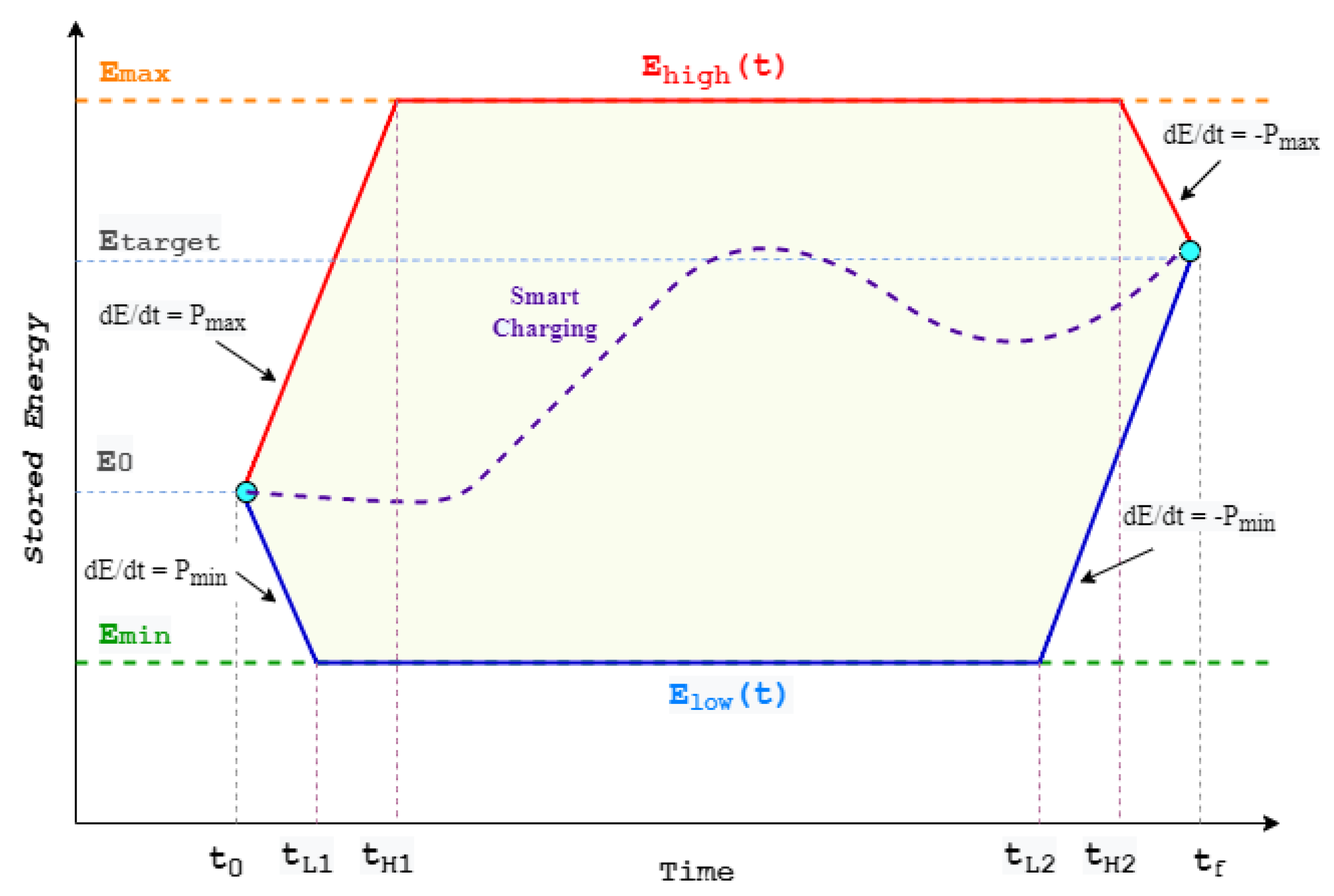
3.3. Parking Dynamic Aggregate Battery Model

A dynamic equivalent battery model was developed for the PEVs that are hosted by a microgrid’s parking lots. It is based on the forecasts of the PEVs’ plug-in and dwell times, their initial stored energy and their batteries’ technical characteristics. The permissible operation area of an individual PEV is shown in Figure 2.

The times that the EV is plugged into the network and unplugged from it are denoted with $t_0$ and $t_f$, respectively. $E_{max}$ and $E_{min}$ are the maximum and the minimum values of a PEV’s battery stored energy (in kWh). $E_0$ is the initial stored energy (kWh) of each PEV. $P_{max}$ and $P_{min}$ are the maximum and minimum power levels that the PEV’s battery can exchange with the network, respectively. $E_{target}$ is the stored energy target that the driver has requested that their PEV should reach at its disconnection time. The dynamic lower and upper bounds of the PEV’s stored energy, $E_{low}$ and $E_{high}$, are generally defined by four points at which they start to decrease or increase with a constant rate of change $P_{min}$ or $P_{max}$. These points are ($t_0$, $E_0$), ($t_{L_1}$, $E_{min}$), ($t_{L_2}$, $E_{min}$) and ($t_f$, $E_{target}$) for $E_{low}$ and ($t_0$, $E_0$), ($t_{H_1}$, $E_{max}$), ($t_{H_2}$, $E_{max}$) and ($t_f$, $E_{target}$) for $E_{high}$ and they are shown in Figure 2.

The variables $t_{L_1}$, $t_{H_1}$_, $t_{L_2}$ and $t_{H_2}$ are estimated as follows [29]:

$$t_{L_1}\left(i\right)=t_0\left(i\right)+\frac{E_{min}\left(i\right)-E_0\left(i\right)}{P_{min}\left(i\right)}$$

(13)

$$t_{H_1}\left(i\right)=t_0\left(i\right)+\frac{E_{max}\left(i\right)-E_0\left(i\right)}{P_{max}\left(i\right)}$$

(14)

$$t_{L_2}\left(i\right)=t_f\left(i\right)+\frac{E_{target}\left(i\right)-E_{min}\left(i\right)}{P_{min}\left(i\right)}$$

(15)

$$t_{H_2}\left(i\right)=t_f\left(i\right)+\frac{E_{target}\left(i\right)-E_{max}\left(i\right)}{P_{max}\left(i\right)}$$

(16)

The $E_{high}$ and $E_{low}$ limits of the $i\mathrm{th}$ PEV are estimated at time t as:

$$E_{high}\left(i,t\right)=\left\{\begin{array}{cc}\hfill E_{max}\left(i\right) ,& \hspace{1em}{t}_{H_1}\left(i\right)\le t\le t_{H_2}\left(i\right)\hfill \\ \hfill E_{max}\left(i\right)-P_{max}\left(t-t_{H_2}(i)\right) ,& \hspace{1em}{t}_{H_2}\left(i\right)<t<t_f\left(i\right)\hfill \\ \hfill E_0\left(i\right)+P_{max}\left(t-t_0(i)\right) ,& \hspace{1em}{t}_0\left(i\right)<t<t_{H1}\left(i\right)\hfill \end{array}\right.$$

(17)

$$E_{low}\left(i,t\right)=\left\{\begin{array}{cc}\hfill E_{min}\left(i\right) ,& \hspace{1em}{t}_{L_1}\left(i\right)\le t\le t_{L_2}\left(i\right)\hfill \\ \hfill E_{min}\left(i\right)+P_{max}\left(t-t_{L_2}(i)\right) ,& \hspace{1em}{t}_{L_2}\left(i\right)<t<t_f\left(i\right)\hfill \\ \hfill E_0\left(i\right)-P_{max}\left(t-t_0(i)\right) ,& \hspace{1em}{t}_0\left(i\right)<t<t_{L1}\left(i\right)\hfill \end{array}\right.$$

(18)

The main goal of the PEV aggregation model is to obtain the dynamic upper and lower limits of the total amount of stored energy in their battery packs and the total active power that they can exchange with the electric network. The time varying technical limits of the equivalent aggregate battery are calculated by applying the following equations:

$$P_{PB,max}\left(t\right)={\displaystyle \sum }_i{P}_{max}\left(i,t\right)$$

(19)

$$P_{PB,min}\left(t\right)={\displaystyle \sum }_i{P}_{min}\left(i,t\right)$$

(20)

$$E_{PB,max}\left(t\right)={\displaystyle \sum }_i{E}_{high}\left(i,t\right)-E_{diff}\left(t\right)$$

(21)

$$E_{PB,min}\left(t\right)={\displaystyle \sum }_i{E}_{low}\left(i,t\right)-E_{diff}\left(t\right)$$

(22)

It should also be noted that the stored energy of the parking-equivalent battery changes continuously due to the continuous plugging and unplugging of the EVs. This change is denoted by $E_{diff}$ and it is calculated by applying the following equations:

$$E_{diff}\left(t\right)={\displaystyle \sum }_{T_0:\Delta t:t} (E_{0,PB}\left(t\right)-E_{t,PB}\left(t\right))$$

(23)

$$E_{0,PB}\left(t\right)={\displaystyle \sum }_{\forall ith EV plugged at t}{E}_0\left(i\right)$$

(24)

$$E_{t,PB}\left(t\right)={\displaystyle \sum }_{\forall ith EV unplugged at t}{E}_{target}\left(i\right)$$

(25)

Let us assume that $P_{opt}\left(t\right)$ is the optimal active power that the equivalent aggregate battery exchanges with the electric network. By adopting generator convention, the resulting stored energy (in kWh) at the end of the next time interval is calculated as it follows:

$$E_{PB}\left(t\right)=E_{PB}\left(T_0\right)-{\displaystyle \sum }_{\Delta t:\Delta t:t}\left\{ch\left(t\right)·P_{opt}\left(t\right)·n_{ch}-\left(1-ch\left(t\right)\right)·\frac{P_{opt}\left(t\right)}{n_{disch}}\right\}·\mathsf{\Delta }t$$

(26)

3.4. Operation Scheduling of the Diesel Generator Set

The optimal operation scheduling of the diesel generators of the buildings can further decrease the operational cost of the microgrid of building prosumers. The generator fuel cost function FC depends on the power that is produced by the generator $P_g$ and it may be accurately approximated by the use of second-order polynomials [30]. Thus, the fuel cost of the gth diesel generator at time t is given as,

$$F{C}_g\left(P_g\left(t\right)\right)=a_{0g}+a_{1g}·P_g\left(t\right)+a_{2g}·P_g{\left(t\right)}^2$$

(27)

4. Optimization Concept

In this work, particle swarm optimization (PSO) has been used in order to optimally schedule the operation of the examined system. It is one of the most highly efficient heuristic methods and it is remarkably simple to implement. PSO has proved very robust and efficient for application to complex optimization problems as it does not depend on the selected initial starting point and leads to a global optimum with a high rate of success.

4.1. First Stage of Optimization

In the first stage of optimization, the algorithm aims to minimize the total operational cost of the microgrid while satisfying all of the associated technical and operation constraints. The decision variables of the examined optimization problem are the following:

• The total HVAC power consumption of each building at every timeslot of the optimization period, $P_{EC,total,b}$.
• The adjustment coefficient of the non-critical electrical loads of each building at each time interval, $n_{shift}$_.
• The state of operation of the gth diesel generator, $s{t}_g$.
• The active power that is exchanged by each PEV parking lot and the microgrid, $P_{opt}\left(t\right)$.
• The active power that is exchanged by the microgrid and the electric grid, $P_{MG}$.

The objective function that is used in this optimization stage and all of the associated constraints is provided next.

$$T{C}_{MG}=\underset{\begin{array}{c}s{t}_g,P_{opt},P_{MG},\\ P_{EC,total},n_{shift}\end{array}}{min}\left\{\left({\displaystyle \sum }_t{P}_{MG}\left(t\right)·EP\left(t\right)+{\displaystyle \sum }_t{\displaystyle \sum }_{g\in \mathcal{G}}s{t}_g\left(t\right)·F{C}_g\left(P_g\left(t\right)\right)\right)·\mathsf{\Delta }t\right\}$$

(28)

s.t.

• Power Balance Constraints

  $$\begin{gathered} {\displaystyle \sum }_{b\in \mathcal{B}}\left(P_{EC,total,b}\left(t\right)+P_{el,b}\left(t\right)\right)= \\ s{t}_{MG}\left(t\right)·P_{MG}\left(t\right)+P_{opt}\left(t\right)+P_{PV}\left(t\right)+P_{WT}\left(t\right)+{\displaystyle \sum }_{g\in \mathcal{G}}s{t}_g\left(t\right)·P_g\left(t\right)) \end{gathered}$$

  (29)

  with

  $$s{t}_{MG}\left(t\right)=\left\{\begin{array}{c}0,\hspace{1em}\hspace{1em}\hspace{1em}\forall t\in \left[T_{auto,0} T_{auto,f}\right]\hfill \\ 1,\hspace{1em}\hspace{1em}\hspace{1em}otherwise\hfill \end{array}\right.$$

  (30)

  $$P_{MG,min}\le P_{MG}\left(t\right)\le P_{MG,max}$$

  (31)
• Building Thermal Load Constraints

  $$T_{min,z}\le T_{in,z}\left(t\right)\le T_{max,z}$$

  (32)

  $$P_{EC,total,min}\le P_{EC,total}\left(t\right)\le P_{EC,total,max}$$

  (33)

  with

  $$P_{EC,z}=\frac{Q_{EC,z}}{COP},\hspace{1em}{P}_{EC,total}=\frac{Q_{EC,total}}{COP}$$

  (34)

  $$Q_{EC,z}\left(t\right)=\frac{\frac{T_{in,z}\left(t\right)-T_{min,z}}{T_{max,z}-T_{min,z}}·V_z}{{\sum }_z\left\{\frac{T_{in,z}\left(t\right)-T_{min,z}}{T_{max,z}-T_{min,z}}·V_z\right\}}·Q_{EC,total}\left(t\right)$$

  (35)

Considering a summer cooling scenario, the power dispatch to the thermal zones is formulated in (35).

• Building Electrical Load Constraints

  $$n_{shift,min} \le n_{shift}\le n_{shift,max}$$

  (36)

  $${\displaystyle \sum }_{t={{\rm T}}_{shift,0}}^{{{\rm T}}_{shift,f}}{P}_{non\_cr}\left(t\right)·\Delta t={\displaystyle \sum }_{t={{\rm T}}_{shift,0}}^{{{\rm T}}_{shift,f}}{P}_{non\_cr}^{*}\left(t\right)·\Delta t$$

  (37)
• Constraints of the Dynamic Aggregate Battery

  $$E_{PB}\left(T_0\right)=E_{PB}\left(T_f\right)$$

  (38)

  $$E_{PB,min}\left(t\right)\le E_{PB}\left(t\right)\le E_{PB,max}\left(t\right)\hspace{1em}\hspace{1em}\forall t\in \left[T_0 T_f\right]$$

  (39)

  $$P_{PB,min}\left(t\right)\le P_{opt}\left(t\right)\le P_{PB,max}\left(t\right)\hspace{1em}\hspace{1em}\forall t\in \left[T_0 T_f\right]$$

  (40)
• Diesel Generator Set Constraints

  $$s{t}_g\left(t\right)·P_{g,min}\le P_g\left(t\right)\le s{t}_g\left(t\right)·P_{g,max},\hspace{1em}\forall t,g$$

  (41)

  $$t_{OFF,g}-t_{ON,g} \ge T_{ON\_min,g} ,\hspace{1em}\forall g$$

  (42)

  $$t_{ON,g}-t_{OFF,g} \ge T_{OFF\_min,g} ,\hspace{1em}\forall g$$

  (43)

4.2. Second Stage of Optimization

In the second optimization stage, the algorithm aims to minimize the total operational cost of the active distribution network by appropriately choosing the adjustment coefficient $n_{DN\_sh}$. The optimal load shifting algorithm is permitted to transfer a certain percentage of the flexible load of one timeslot to a different one, provided that the energy that is consumed before and after the load shifting remains the same.

It is considered that the electrical power consumption of the flexible loads constitutes a percentage of the overall power that is consumed by the electrical loads of the distribution network ($P_{DN,load})$.

The objective function that is used in this optimization stage is formulated in (44). It aims to minimize the operational cost of the active distribution network by suitable load shifting. Network constraints are not considered in this stage.

$$\begin{array}{cc} \hfill & \hspace{1em}\hspace{1em}T{C}_{DN}=\underset{n_{DN\_sh}}{min}\left\{\left({\displaystyle \sum _t}{P}_{DN}\left(t\right)·EP\left(t\right)\right)·\Delta t\right\}\hfill \\ \mathrm{subject} \mathrm{to}\hfill & \hfill \end{array}$$

(44)

• Flexible Electrical Load Constraints

  $$P_{DN,flex}^{*}\left(t\right)=\left\{\begin{array}{cc}{n}_{DN\_sh}\left(t\right)·P_{DN,flex}\left(t\right),\hfill & \hspace{1em}\forall t \in \left[{{\rm T}}_{DN\_sh,0} {{\rm T}}_{DN\_sh,f}\right]\hfill \\ \hspace{1em}\hspace{1em}\hspace{1em}\hspace{1em}\hspace{1em}{P}_{DN,flex}\left(t\right),\hfill & \hspace{1em}otherwise\hfill \end{array}\right.$$

  (45)

  $$n_{DN\_sh,min} \le n_{DN\_sh}\le n_{DN\_sh,max}$$

  (46)

  $${\displaystyle \sum }_{t={{\rm T}}_{DN\_sh,0}}^{{{\rm T}}_{DN\_sh,f}}{P}_{DN,flex}\left(t\right)·\Delta t={\displaystyle \sum }_{t={{\rm T}}_{DN\_sh,0}}^{{{\rm T}}_{DN\_sh,f}}{P}_{DN,flex}^{*}\left(t\right)·\Delta t$$

  (47)
• Power Balance Constraints

  $$P_{DN,load}\left(t\right)+s{t}_{MG}\left(t\right)·P_{MG}\left(t\right)=s{t}_{DN}\left(t\right)·P_{DN}\left(t\right)+P_{PV}\left(t\right)+P_{WT}\left(t\right)\hspace{1em}\forall t\in \left[T_0 T_f\right]$$

  (48)

  with

  $$P_{DN,flex}\left(t\right)=n_{flex}·P_{DN,load}\left(t\right)$$

  (49)

  $$P_{DN,load}\left(t\right)=P_{DN,non\_flex}\left(t\right)+P_{DN,flex}^{*}\left(t\right)$$

  (50)

  $$P_{DN,min}\le P_{DN}\left(t\right)\le P_{DN,max}$$

  (51)

4.3. Third Stage of Optimization

In this optimization stage, the deviations of the building’s electric consumption $\Delta P_{buildings}$, diesel generator power $\Delta P_{diesel}$ and PEV parking lot power $\Delta P_{PEVs,aggr}$ from their optimal values are estimated. These optimal values are those that lead to the maximum deviations of the power that the microgrid exchanges with the active distribution network that contributes to all of the network constraint violation elimination processes and ensures satisfaction of all of the microgrid constraints. The objective function that is used in the third stage of optimization is provided in (52), followed by its respective constraints.

$$\underset{\begin{array}{c}\Delta P_{buildings},\\ \Delta P_{diesel}\\ \Delta P_{PEVs,aggr}\end{array}}{max}\left\{{\displaystyle \sum }_{t={\underset{\_}{T}}_{reg, V\downarrow }}^{{\overline{T}}_{reg, V\downarrow }}\left|\Delta P_{MG}\left(t\right)\right|+{\displaystyle \sum }_{t={\underset{\_}{T}}_{reg, V\uparrow }}^{{\overline{T}}_{reg, V\uparrow }}\left|\Delta P_{MG}\left(t\right)\right|\right\}$$

(52)

s.t. (32)–(43) and

$$\Delta P_{buildings}\left(t\right)+\Delta P_{diesel}\left(t\right)+\Delta P_{PEVs,aggr}=\Delta P_{MG}\left(t\right)$$

(53)

$$\Delta P_{buildings,min}\le \Delta P_{buildings}\left(t\right)\le \Delta P_{buildings,max}\hspace{1em}\hspace{1em}\hspace{1em}\hspace{1em}t\notin \left[{\underset{\_}{T}}_{reg, V\downarrow } {\overline{T}}_{reg, V\downarrow }\right],\hspace{1em}\left[{\underset{\_}{T}}_{reg, V\uparrow } {\overline{T}}_{reg, V\uparrow }\right]$$

(54)

$$\Delta P_{buildings,min}\le \Delta P_{buildings}\left(t\right)\le 0\hspace{1em}\hspace{1em}\hspace{1em}\hspace{1em}t\in \left[{\underset{\_}{T}}_{reg, V\downarrow } {\overline{T}}_{reg, V\downarrow }\right]$$

(55)

$$0\le \Delta P_{buildings}\left(t\right)\le \Delta P_{buildings,max}\hspace{1em}\hspace{1em}t\in \left[{\underset{\_}{T}}_{reg, V\uparrow } {\overline{T}}_{reg, V\uparrow }\right]$$

(56)

$$\Delta P_{diesel,min}\le \Delta P_{diesel}\left(t\right)\le \Delta P_{diesel,max}\hspace{1em}\hspace{1em}\hspace{1em}\hspace{1em}t\notin \left[{\underset{\_}{T}}_{reg, V\downarrow } {\overline{T}}_{reg, V\downarrow }\right],\hspace{1em}\left[{\underset{\_}{T}}_{reg, V\uparrow } {\overline{T}}_{reg, V\uparrow }\right]$$

(57)

$$0\le \Delta P_{diesel}\left(t\right)\le \Delta P_{diesel,max}\hspace{1em}\hspace{1em}\hspace{1em}\hspace{1em}t\in \left[{\underset{\_}{T}}_{reg, V\downarrow } {\overline{T}}_{reg, V\downarrow }\right]$$

(58)

$$\Delta P_{diesel,min}\le \Delta P_{diesel}\left(t\right)\le 0\hspace{1em}\hspace{1em}t\in \left[{\underset{\_}{T}}_{reg, V\uparrow } {\overline{T}}_{reg, V\uparrow }\right]$$

(59)

$$\Delta P_{PEVs,aggr,min}\le \Delta P_{PEVs,aggr}\left(t\right)\le \Delta P_{PEVs,aggr,max}\hspace{1em}\hspace{1em}\hspace{1em}\hspace{1em}t\notin \left[{\underset{\_}{T}}_{reg, V\downarrow } {\overline{T}}_{reg, V\downarrow }\right],\hspace{1em}\left[{\underset{\_}{T}}_{reg, V\uparrow } {\overline{T}}_{reg, V\uparrow }\right]$$

(60)

$$\Delta P_{PEVs,aggr,min}\le \Delta P_{PEVs,aggr}\left(t\right)\le 0\hspace{1em}\hspace{1em}\hspace{1em}\hspace{1em}t\in \left[{\underset{\_}{T}}_{reg, V\downarrow } {\overline{T}}_{reg, V\downarrow }\right]$$

(61)

$$0\le \Delta P_{PEVs,aggr}\left(t\right)\le \Delta P_{PEVs,aggr,max}\hspace{1em}\hspace{1em}t\in \left[{\underset{\_}{T}}_{reg, V\uparrow } {\overline{T}}_{reg, V\uparrow }\right]$$

(62)

4.4. Fourth Stage of Optimization

The objective function of this optimization stage is formulated in (63).

$$T{C}_{DN}=\underset{\begin{array}{c}{n}_{D{N}_{sh}},\\ P_{MG}\end{array}}{min}\left\{\left({\displaystyle \sum }_t{P}_{DN}\left(t\right)·EP\left(t\right)\right)·\Delta t\right\}$$

(63)

s.t. (45)–(51) and

• Active Distribution Network Constraints

$$\mathit{V}·\overline{\mathit{Y}}·\overline{\mathit{V}}={\mathit{S}}_{inj}={\mathit{P}}_{inj}+j·{\mathit{Q}}_{inj}$$

(64)

$$\left|\mathit{V}\left(k,t\right)\right|\le {\mathit{V}}_{max}\left(k\right)$$

(65)

$$\left|\mathit{V}\left(k,t\right)\right|\ge {\mathit{V}}_{min}\left(k\right)$$

(66)

$$\mathbf{\theta }\left(k,t\right)\ge {\mathbf{\theta }}_{min}\left(k\right)$$

(67)

$$\mathbf{\theta }\left(k,t\right)\le {\mathbf{\theta }}_{max}\left(k\right)$$

(68)

$$\left|\mathit{Y}\left(k,l\right)·\left(\mathit{V}\left(k,t\right)-\mathit{V}\left(l,t\right)\right)\right|\le {\mathit{I}}_{max}\left(k,l\right)$$

(69)

where $\mathit{V}$ and $\mathbf{\theta }$ are vectors representing the amplitudes and the angles of the distribution network voltages and $\mathit{Y}$ is the network admittance matrix. The variable $\left|\mathit{V}\left(k\right)\right|$ is the voltage amplitude at the $kth$ node, $\mathbf{\theta }\left(k\right)$ is voltage angle at the $kth$ node and ${\mathit{I}}_{max}\left(k,l\right)$ is the maximum current flowing in the electric line connecting the $kth$ and $lth$ node. The ${\mathit{S}}_{inj}$ vector comprises the apparent power injections at the nodes of the network while ${\mathit{P}}_{inj}$ and ${\mathit{Q}}_{inj}$ comprise the active and reactive power injections at all of the network nodes, respectively.

MatPower was used to solve the optimal power flow (OPF) problem with the constraints that are defined in (64)–(69) [31]. MatPower uses the solvers of non-linear constrained optimization problems that are provided in the Matlab Optimization Toolbox in order to solve the AC OPF problem and it can deal with the most constraints that are associated with the electrical network’s operation.

4.5. Fifth Stage of Optimization

The decision variables in this stage are the first four that are described in the first optimization level. The objective function that is used in this optimization stage is provided in (70).

$$\begin{array}{c}\hspace{1em}\hspace{1em}\hspace{1em}\hspace{1em}\hspace{1em}T{C}_{MG}=\underset{\begin{array}{c}s{t}_g,P_{opt},\\ P_{EC,total},n_{shift}\end{array}}{min}\left\{\left({\displaystyle \sum _t}{\displaystyle \sum _{g\in \mathcal{G}}}s{t}_g\left(t\right)·F{C}_g\left(P_g\left(t\right)\right)\right)·\Delta t\right\}\hfill \\ \mathrm{s}.\mathrm{t}. \left(29\right)–\left(43\right)\hfill \end{array}$$

(70)

The power that is exchanged by the microgrid and the active distribution network is required to be equal to that which was obtained in the fourth optimization level.

5. Case Study

In the examined case study, the microgrid was assumed to comprise three large office buildings, three large EV parking lots, two auxiliary diesel generators, two PV parks and one wind turbine park. The IEEE 33-node radial distribution network has been used as the electric network in the proposed system. The single-line diagram of the examined electric distribution network is shown in Figure 3.

The model parameters that are related to the buildings of the microgrid are tabulated in

Table 1. Thermal zones’ characteristics.

	Building 1	Building 2	Building 3
Side_1 (m)	10	12	10
Side_2 (m)	20	20	20
Height (m)	3	3	3
Tmin/Tmax (°C)	19/27.5	19/27.5	19/27.5

,

Table 2. Thermal zones’ parameters.

${\mathit{p}}_{\mathit{z}}\left(\mathrm{kg}/m^3\right)$	$1.2$
${\mathit{C}}_{\mathit{z}}\left(\mathrm{kWh}/\left(\mathrm{kg}·°C\right)\right)$	$1/3600$
${\mathit{U}}_{\mathit{wall},\mathit{z}}\left(kW/\left(m^2·°C\right)\right)$	$2.04·{10}^{-3}$
${\mathit{U}}_{\mathit{win},\mathit{z}}\left(kW/\left(m^2·°C\right)\right)$	$5.6·{10}^{-3}$
${\tau }_{\mathit{win},\mathit{z}}$	$1.1·{10}^{-3}$
${\mathit{a}}_{\mathit{w},\mathit{z}}$	$0.2$
$\mathit{S}{\mathit{C}}_{\mathit{z}}$	$0.54$
${\mathit{p}}_{\mathit{g}}$	$0.2$
${\mathit{\beta }}_{\mathit{z}}\left(°\right)$	$90$
$\mathit{\theta }\left(°\right)$	$11.9$
${\mathit{\theta }}_{\mathit{z}}\left(°\right)$	$39.9$
${\mathit{R}}_{\mathit{se},\mathit{z}}\left(\left(m^2·°C\right)/kW\right)$	$40$

,

Table 3. Building parameters.

	Building 1	Building 2	Building 3
Number of floors	15	25	35
Total number of thermal zones	90	225	385

and

Table 4. Non-critical loads’ parameters.

	Building 1	Building 2	Building 3
$n_{non\_cr}$	0.25	0.25	0.25
$n_{shift,min}$	0.70	0.75	0.65
$n_{shift,max}$	1.3	1.25	1.35
$T_{shift,min}$	07:00	07:00	07:00
$T_{shift,max}$	17:00	17:00	17:00

. Four types of PEV batteries were considered in this article with their technical characteristics given in

Table 5. PEVs’ parameters.

	PEV Type
	1	2	3	4
$Battery Capacity\left(\mathrm{kWh}\right)$	77	45	26.8	66.5
$So{C}_{max}/So{C}_{min} \left(\mathrm{kWh}\right)$	69.3/7.7	40.5/4.5	24.12/2.7	60/6.65
$P_{max}/P_{min} \left(\mathrm{kW}\right)$	11/−11	7.2/−7.2	6.6/−6.6	11/−11

. All of the necessary technical parameters of the diesel generators are presented in

Table 6. Diesel generators’ model data.

	GEN1	GEN2
Technical minimum (kW)	285	600
Technical maximum (kW)	1000	2100
Minimum hours for generator being in operation/out of operation (h)	1/1	1/1
Cost of consumed fuel (m.u./h)	$62.8-0.1114·P+$ $\dots +2·{10}^{-4}·P^2$	$137-0.122·P+$ $\dots +8·{10}^{-5}·P^2$

.

The ambient temperature that was used in this case study is shown in Figure 4 and it is a typical daily temperature time series from late summer in Greece. The time series of the electricity price forecast that was used in the examined scenario is shown in Figure 5. It was assumed that the electricity price that was forecast was carried out by the power system operator and provided to the microgrid and the active distribution network. Provided that the computation time that is required by the proposed method is small (of the scale of a few minutes), it was assumed that the electricity price forecast would be provided to the local electricity market participants after the day-ahead electricity market was carried out.

The number of people conducting activity in each building of the microgrid is shown in Figure 6. As can be seen in this figure, the maximum number of active people in each building were present from 13:00–14:00.

The connection and the dwell periods of the PEVs rely on the different types of activities (being at home, being at work, shopping and social engagements) that their drivers partake in and they are calculated using their respective probability density functions (PDFs) [32], as are shown in Figure 7a and Figure 7b, respectively. For instance, as it can be observed, the connection rate for the PEVs of citizens who are at work peaked at 7:30 a.m., whereas their dwell time peaked at approximately 8.5 h. The obtained total number of the connected EVs that were found during the examined time period is shown in Figure 8.

The time series of the power generation of Photovoltaics (PVs) and Wind Turbines ( WTs) are shown in Figure 9.

The internal temperatures of all of the buildings’ thermal zones that are obtained in the first optimization level, with their upper and lower bounds, are given in Figure 10. It was observed that the internal temperatures of all of the thermal zones of each building were consistently well-maintained between the comfortable temperature range of 19–27.5 °C and they all tended to behave in the same way.

The electric power consumptions of the HVAC systems of the buildings are shown in Figure 11. As anticipated, each building’s total cooling power changed according to the ambient temperature and the predicted pattern of occupant activity. Obviously, the largest building had the biggest cooling needs. The algorithm aims to reduce the power demand when the electricity price is quite high.

The total non-critical electrical demand of the buildings of the microgrid is shown in Figure 12, before and after the first level of optimization was implemented. It can be noted that the algorithm optimally shifted the non-critical electrical loads from the high electricity time period to the time period from 13:00–16:00, when the electricity price was low.

Figure 13 exhibits the power that was produced by the diesel generators. The generators were scheduled to operate as close as possible to their optimal operation point.

The total active power of the PEV parking lot, together with its respective upper and lower limits, is shown in Figure 14. Generator convention was used, hence the negative values indicate that the aggregate battery absorbed power from the grid (i.e., it was charging), while positive values indicate that the battery injected power to the grid (i.e., it was discharging). The total energy that was stored in the equivalent aggregate battery of the microgrid’s parking lot, as well as its respective upper and the lower limits, is shown in Figure 15. These limits changed over time as a result of the fluctuating number of connected EVs and electricity price variations. The algorithm effectively covered the microgrid’s energy demand with internal power sources during its autonomous operation and, at the same time, it reduced its daily operational cost. It was observed that all of the PEVs managed to reach their energy targets while satisfying all of the operational and technical constraints. In order to guarantee that the necessary energy was stored during the microgrid’s island operation, the PEVs were compelled to store extra energy from the electric grid before the grid’s power supply was interrupted.

The time series of all of the node voltages after the execution of optimization stage 2 are shown in Figure 16. The upper and lower voltage limits were set to 1.1 and 0.9 p.u., respectively. According to Figure 16, the voltages of the network buses were out of the predefined limits during the time period from 19:00–22:00.

Therefore, it was necessary to identify the time periods during which the network constraints were violated and provide them to the microgrid in order to evaluate the minimum and maximum possible deviations of its power exchange in optimization stage 3, as is shown in Figure 17. It was considered that the maximum permitted fluctuations of the power of the buildings, parking lots’ aggregate battery and diesel generators were up to 20% of their installed power capacity. At the same time, as can be observed in Figure 18, the internal temperatures of all of the thermal zones of the buildings were well-maintained between their minimum and maximum limits.

In the time period from 19:00–22:00, when the voltages of the distribution network nodes dropped, the cooling power of the buildings was required to be reduced (as is shown in Figure 17) and, therefore, the indoor temperatures of the buildings increased.

Moreover, Figure 17 exhibits the optimal deviation of the power that was exchanged between the microgrid and the active distribution network as was obtained from optimization stage 4. It is obvious that it was within its predefined bounds. Figure 19 exhibits the active distribution network load before and after optimization stages 2 and 4 were implemented. In the second optimization stage, it was observed that the flexible electrical loads were shifted to time periods of low electricity price (13:00–15:00) in order to contribute to the minimization of the active distribution network’s total operational cost while satisfying all of the operational constraints at the same time. The time series of all of the node voltages after the execution of optimization stage 2 are shown in Figure 20. It can be seen that the distribution network voltages were well-maintained within their permissible limits.

Figure 21 exhibits the power that was exchanged between the microgrid and the active distribution network after the execution of optimization levels 1 and 4.

6. Discussion

In this paper, a method for the coordinated optimal operation scheduling of active distribution networks hosting complex microgrids comprising large building prosumers and plug-in electric vehicle aggregators is proposed. The operational costs of both the microgrid and active distribution network were optimized while all of the associated constraints were fully satisfied. The proposed method is suitable to handle very complex microgrids comprising large building prosumers and a large number of PEVs. An aggregation technique was used to handle the large number of PEVs and a simple thermal power dispatch technique was used for the efficient modelling of the large building prosumers. A modified IEEE 33-bus test case system was used to test the efficiency of the proposed method. The obtained simulation results show that the proposed method led to the optimization of the operational costs of both the active distribution network and the microgrid while it ensured adherence to a large set of operation constraints of the microgrid and the active distribution network. As a future extension of this work, a method for the optimal real-time operation of the electrical and thermal energy systems of the buildings end energy storage facilities can be developed in order to effectively deal with the uncertainties arising from the predictions of stochastic variables, such as the price of electricity, the production of renewable energy sources and the activity of people and the hosted electric vehicles.

References

1. Thomas, D.; Deblecker, O.; Ioakimidis, C.S. Optimal operation of an energy management system for a grid-connected smart building considering photovoltaics’ uncertainty and stochastic electric vehicles’ driving schedule. Appl. Energy 2018, 210, 1188–1206. [Google Scholar] [CrossRef]
2. Sturzenegger, D.; Gyalistras, D.; Morari, M.; Smith, R.S. Model Predictive Climate Control of a Swiss Office Building: Implementation, Results, and Cost-Benefit Analysis. IEEE Trans. Control. Syst. Technol. 2016, 24, 1–12. [Google Scholar] [CrossRef]
3. Carli, R.; Dotoli, M. Decentralized control for residential energy management of a smart users’ microgrid with renewable energy exchange. IEEE/CAA J. Autom. Sin. 2019, 6, 641–656. [Google Scholar] [CrossRef]
4. Alibabaei, N.; Fung, A.S.; Raahemifar, K.; Moghimi, A. Effects of intelligent strategy planning models on residential HVAC system energy demand and cost during the heating and cooling seasons. Appl. Energy 2017, 185, 29–43. [Google Scholar] [CrossRef]
5. Akter, M.N.; Mahmud, M.A.; Oo, A.M.T. A hierarchical transactive energy management system for energy sharing in residential microgrids. Energies 2017, 10, 2098. [Google Scholar] [CrossRef]
6. Jiang, Q.; Xue, M.; Geng, G. Energy management of microgrid in grid-connected and stand-alone modes. IEEE Trans. Power Syst. 2013, 28, 3380–3389. [Google Scholar] [CrossRef]
7. Li, Z.; Xu, Y. Optimal coordinated energy dispatch of a multi-energy microgrid in grid-connected and islanded modes. Appl. Energy 2018, 210, 974–986. [Google Scholar] [CrossRef]
8. Worku, M.Y.; Hassan, M.A.; Abido, M.A. Real time energy management and control of renewable energy based microgrid in grid connected and Island modes. Energies 2019, 12, 276. [Google Scholar] [CrossRef]
9. Zheng, Y.; Li, S.; Tan, R. Distributed Model Predictive Control for On-Connected Microgrid Power Management. IEEE Trans. Control. Syst. Technol. 2018, 26, 1028–1039. [Google Scholar] [CrossRef]
10. Zhang, Y.; Gatsis, N.; Giannakis, G.B. Robust energy management for microgrids with high-penetration renewables. IEEE Trans. Sustain. Energy 2013, 4, 944–953. [Google Scholar] [CrossRef] [Green Version]
11. Pinzon, J.A.; Vergara, P.P.; da Silva, L.C.P.; Rider, M.J. Optimal Management of Energy Consumption and Comfort for Smart Buildings Operating in a Microgrid. IEEE Trans. Smart Grid 2019, 10, 3236–3247. [Google Scholar] [CrossRef]
12. Pinzon, J.A.; Vergara, P.P.; da Silva, L.C.P.; Rider, M.J. A MILP model for optimal management of energy consumption and comfort in smart buildings. In Proceedings of the 2017 IEEE Power and Energy Society Innovative Smart Grid Technologies Conference, ISGT, Arlington, VA, USA, 23–26 April 2017. [Google Scholar]
13. Hao, H.; Corbin, C.D.; Kalsi, K.; Pratt, R.G. Transactive Control of Commercial Buildings for Demand Response. IEEE Trans. Power Syst. 2017, 32, 774–783. [Google Scholar] [CrossRef]
14. Bharati, G.R.; Razmara, M.; Paudyal, S.; Shahbakhti, M.; Robinett, R.D. Hierarchical optimization framework for demand dispatch in building-grid systems. In Proceedings of the IEEE Power and Energy Society General Meeting, Boston, MA, USA, 17–21 July 2016. [Google Scholar]
15. Tavakoli, M.; Shokridehaki, F.; Marzband, M.; Godina, R.; Pouresmaeil, E. A two stage hierarchical control approach for the optimal energy management in commercial building microgrids based on local wind power and PEVs. Sustain. Cities Soc. 2018, 41, 332–340. [Google Scholar] [CrossRef]
16. Sehar, F.; Pipattanasomporn, M.; Rahman, S. Coordinated control of building loads, PVs and ice storage to absorb PEV penetrations. Int. J. Electr. Power Energy Syst. 2018, 95, 394–404. [Google Scholar] [CrossRef]
17. Liang, Z.; Bian, D.; Zhang, X.; Shi, D.; Diao, R.; Wang, Z. Optimal energy management for commercial buildings considering comprehensive comfort levels in a retail electricity market. Appl. Energy 2019, 236, 916–926. [Google Scholar] [CrossRef]
18. Dakanalis, M.; Kanellos, F.D. Efficient model for accurate assessment of frequency support by large populations of plug-in electric vehicles. Inventions 2021, 6, 89. [Google Scholar] [CrossRef]
19. Liu, Z.; Chen, Y.; Zhuo, R.; Jia, H. Energy storage capacity optimization for autonomy microgrid considering CHP and EV scheduling. Appl. Energy 2018, 210, 1113–1125. [Google Scholar] [CrossRef]
20. Lan, T.; Jermsittiparsert, K.; Alrashood STRezaei MAl-Ghussain, L.; Mohamed, M.A. An advanced machine learning based energy management of renewable microgrids considering hybrid electric vehicles’ charging demand. Energies 2021, 14, 569. [Google Scholar] [CrossRef]
21. Han, Y.; Chen, W.; Li, Q. Energy management strategy based on multiple operating states for a photovoltaic/fuel cell/energy storage DC microgrid. Energies 2017, 10, 136. [Google Scholar] [CrossRef]
22. Eseye, A.T.; Lehtonen, M.; Tukia, T.; Uimonen, S.; Millar, R.J. Optimal Energy Trading for Renewable Energy Integrated Building Microgrids Containing Electric Vehicles and Energy Storage Batteries. IEEE Access 2019, 7, 106092–106101. [Google Scholar] [CrossRef]
23. Anvari-Moghaddam, A.; Rahimi-Kian, A.; Mirian, M.S.; Guerrero, J.M. A multi-agent based energy management solution for integrated buildings and microgrid system. Appl. Energy 2017, 203, 41–56. [Google Scholar] [CrossRef]
24. Li, Y.; Feng, B.; Li, G.; Qi, J.; Zhao, D.; Mu, Y. Optimal distributed generation planning in active distribution networks considering integration of energy storage. Appl. Energy 2018, 210, 1073–1081. [Google Scholar] [CrossRef]
25. Nick, M.; Cherkaoui, R.; Paolone, M. Optimal Planning of Distributed Energy Storage Systems in Active Distribution Networks Embedding Grid Reconfiguration. IEEE Trans. Power Syst. 2018, 33, 1577–1590. [Google Scholar] [CrossRef]
26. Nuchkrua, T.; Leephakpreeda, T. Novel Compliant Control of a Pneumatic Artificial Muscle Driven by Hydrogen Pressure Under a Varying Environment. IEEE Trans. Ind. Electron. 2022, 69, 7120–7129. [Google Scholar] [CrossRef]
27. Jin, X.; Wu, J.; Mu, Y.; Wang, M.; Xu, X.; Jia, H. Hierarchical microgrid energy management in an office building. Appl. Energy 2017, 208, 480–494. [Google Scholar] [CrossRef]
28. Farinis, G.Κ.; Kanellos, F.D. Integrated energy management system for Microgrids of building prosumers. Electr. Power Syst. Res. 2021, 198, 107357. [Google Scholar] [CrossRef]
29. Kanellos, F.D. Optimal Scheduling and Real-Time Operation of Distribution Networks with High Penetration of Plug-In Electric Vehicles. IEEE Syst. J. 2021, 15, 3938–3947. [Google Scholar] [CrossRef]
30. Kanellos, F.D. Optimal power management with GHG emissions limitation in all-electric ship power systems comprising energy storage systems. IEEE Trans. Power Syst. 2014, 29, 330–339. [Google Scholar] [CrossRef]
31. Zimmerman, R.D.; Murillo-Sanchez, C.E.; Thomas, R.J. MATPOWER: Steady-State Operations, Planning, and Analysis Tools for Power Systems Research and Education. IEEE Trans. Power Syst. 2011, 26, 12–19. [Google Scholar] [CrossRef] [Green Version]
32. Santos, A.; McGuckin, N.; Nakamoto, H.Y.; Gray, D.; Liss, S. Summary of Travel Trends: 2009 National Household Travel Survey; U.S. Department Of Transportation, Federal Highway Administration: Washington, DC, USA, 2011. Available online: http://nhts.ornl.gov/2009/pub/stt.pdf (accessed on 24 August 2022).
Figure 1. Configuration of the proposed system.
Energies 15 06182 g001
Figure 2. Bounds of PEV’s stored energy.
Energies 15 06182 g002
Figure 3. Single-line diagram of the examined distribution network.
Energies 15 06182 g003
Figure 4. Ambient temperature.
Energies 15 06182 g004
Figure 5. Electricity price.
Energies 15 06182 g005
Figure 6. Forecasted number of active people in microgrid’s building.
Energies 15 06182 g006
Figure 7. (a) PDF of electric vehicles’ connection time; (b) PDF of electric vehicles’ dwell time.
Energies 15 06182 g007
Figure 8. Number of connected EVs.
Energies 15 06182 g008
Figure 9. Photovoltaic and wind power generation.
Energies 15 06182 g009
Figure 10. Internal temperatures of all buildings’ thermal zones (optimization level 1).
Energies 15 06182 g010
Figure 11. Total cooling power of each building of the microgrid (optimization level 1).
Energies 15 06182 g011
Figure 12. Total non-critical electrical loads before and after the execution of optimization level 1.
Energies 15 06182 g012
Figure 13. Power produced by auxiliary diesel generators (optimization level 1).
Energies 15 06182 g013
Figure 14. Active power of PEV aggregator and its upper and lower bounds.
Energies 15 06182 g014
Figure 15. Total stored energy of PEV aggregator and its upper and lower bound.
Energies 15 06182 g015
Figure 16. Node voltages (optimization level 2).
Energies 15 06182 g016
Figure 17. Optimal deviation of the power transferred between the microgrid and the active distribution network.
Energies 15 06182 g017
Figure 18. Internal temperatures of all building thermal zones (optimization level 3).
Energies 15 06182 g018
Figure 19. Active distribution network load before and after the execution of the optimization levels 2 and 4.
Energies 15 06182 g019
Figure 20. Node voltages (optimization level 4).
Energies 15 06182 g020
Figure 21. Active power exchanged between the microgrid and the active distribution network (optimization levels 1 and 4).
Energies 15 06182 g021