Article

Towards Data-Driven Models in the Prediction of Ship Performance (Speed—Power) in Actual Seas: A Comparative Study between Modern Approaches

by
Kiriakos Alexiou
1,
Efthimios G. Pariotis
2,
Helen C. Leligou
1 and
Theodoros C. Zannis
2,*
1
Department of Industrial Design and Production Engineering, University of West Attica, 12243 Athens, Greece
2
Naval Architecture and Marine Engineering Section, Hellenic Naval Academy, 18539 Piraeus, Greece
*
Author to whom correspondence should be addressed.
Energies 2022, 15(16), 6094; https://doi.org/10.3390/en15166094
Submission received: 6 July 2022 / Revised: 7 August 2022 / Accepted: 16 August 2022 / Published: 22 August 2022
(This article belongs to the Section K: State-of-the-Art Energy Related Technologies)

Abstract

:
In the extremely competitive environment of shipping, minimizing shipping cost is the key factor for the survival and growth of shipping companies. However, stricter rules and regulations that aim at the reduction of greenhouse gas emissions published by the International Maritime Organization, force shipping companies to increase the operational efficiency of their fleet. The prediction of a ship speed in actual seas with a given power by its engine is the most important performance indicator and thus makes it the “holy grail” in pursuing better efficiency. Traditionally, tank model tests and semi-empirical formulas were the preferred solution for the aforementioned prediction and are still widely applied. However, currently, with the increased computational power that is widely available, novel and more sophisticated methods taking into consideration computational fluid dynamics (CFD) and machine learning (ML) algorithms are emerging. In this paper, we briefly present the different approaches in the prediction of a ship’s speed but focus on ML methods comparing a representative number of the latest data-driven models used in papers, to provide guidelines, discover trends and identify the challenges to be faced by researchers. From this comparison, we can distinguish that artificial neural networks (ANN), being used in 73.3% of the reviewed papers, dominate as the algorithm of choice. Researchers mostly rely on physical laws governing the phenomena in the crucial part of data preprocessing tasks. Lastly, most researchers rely on data acquisition systems installed at ships in order to achieve usable results.

1. Introduction

Lately, an ongoing race in the marine industry for the improvement of energy efficiency in ships has been witnessed. Recent events such as the fuel oil crisis that started in 2021 [1], show that the effort to reduce shipping costs is more critical than ever. The cost of fuel has become the dominant factor of the operational cost of the ships. Conversely, the mandatory compliance in new stricter regulations regarding the reduction of greenhouse gas emissions is forcing the industry to search for and adopt methods to optimize the performance of all vessels. The International Maritime Organization (IMO) introduced in 2018 its long-term strategy in order to reduce the environmental footprint of the marine industry. The CO2 gas emissions per transport work must be reduced by 40% compared to the corresponding CO2 gas emissions of 2008, until 2030. The percentage of reduction is increased to 70% by the year 2050 [2]. The key design aspect of new vessels has become the improvement of the Energy Efficiency Design Index (EEDI) [3], while Energy Efficiency Operational Indicator (EEOI) [4], and Ship Energy Efficiency Management Plan (SEEMP) [5], Energy Efficiency Existing Ship Index (EEXI) [6] and Carbon Intensity Indicator (CII) [7] are the corresponding criteria for evaluation of the existing fleet.
The speed that a ship can reach with a given amount of power from the propulsion system is a measure of hull efficiency. Maximizing the ship speed with respect to water, speed through water (STW), while keeping the power of the engine constant, or conversely minimizing the required power for a specific STW, equals to maximizing the energy efficiency of the vessel (regarding propulsion). With this in mind, the adequate estimation (prediction) of ship speed is of utmost importance in the process of reduction/minimization of fuel oil consumption (FOC) of the ship’s engine. The STW of a ship is the result of many factors. Weather conditions, ship resistance, hull degradation, propulsion system efficiency and propeller design characteristics are the most important [8]. The above factors shape the total resistance that marine engines have to overcome to achieve a certain speed.
The accurate estimation of the above resistance components differs in complexity, and many different approaches can be found in the literature. Semi-empirical formulas and model tests are the well-established “traditional” approaches. These methods are well developed and can give accurate estimations for the resistance in calm weather and the added resistance due to wind, but both of them lack the necessary accuracy in the prediction of added resistance due to irregular waves [9]. This weakness forced the scientific community to try different approaches. With the vastly increased computational power that is widely available, more advanced methods for performance estimation are starting to dominate.
Computational fluid dynamics (CFD) and data-driven models are the new trend in the search of accurate prediction of ship performance because these take into account the actual status of the ship (weather conditions, hull degradation, operational profile, propulsion system efficiency and propeller design characteristics), either in detailed level as far as CFD models are concerned or as a whole (black box) in the case of data-driven models. CFD is fundamentally based on physical models and solves the relative equations of mass, energy and momentum conservation at each computational node, using high CPU demanding mathematical procedures for the convergence of the problem. The describing system of partial differential equations is impossible to solve analytically in order to approximate the solutions via numerical algorithms (solvers) that are calculated by computers [10]. CFD can be a highly accurate method for calculating ship resistance and is the preferred one in the design phase of ship building, with an expected error margin of 4% [11]. Using CFD in real weather conditions is a far more complex procedure due to the difficulty in accurately describing the real boundary conditions, which result in increased uncertainty for the accuracy of the predicted values. Concluding, CFD models are based on a solid physical background for the prediction of ship performance, providing detailed information of the ship design, which in most cases remains in the possession of shipyards.
Data-driven approaches have become possible due to the digitization of the maritime industry. All new ships and an increasing number of existing ones are adopting Internet of Things (IoT) platforms that collect and process a vast amount of data from various sensors installed on board [12]. This transformation has paved the way for the entrance of a new trend toward data science. As the research efforts in this direction intensify, the aim of this study is to present the different approaches in estimation of a ship performance focusing on data-driven models. The dominant data-driven models, the algorithms in use and the applied procedures are presented and compared to provide useful insights and guidelines for their appropriate application in real-life cases. There are interesting papers in the literature that compare different ML algorithms and present the data pipeline (method) used for predicting a ship’s speed [13], but the advances in ML dictate the necessity of an updated review in regular intervals. Furthermore, the authors believe that the review of the methodology used by different researchers can represent the trend toward the implementation of these models in ship performance, as long as there are common limitations. For this purpose, fifteen recent studies that are focusing on the era of ship performance prediction using ML algorithms are reviewed. These studies were selected by their association with the subject of the study and by the publication date in order to better represent the modern trend.
The rest of the paper is organized as follows: in Section 2, we briefly present modern papers where researchers access the topic of ship performance prediction in actual seas using semi-empirical formulas, model tests and CFD. In Section 3, data-driven model presentation, the basic theory of the most known and frequently used machine learning algorithms, along with the different metrics of prediction are presented. Section 4 is dedicated to the presentation of some representative modern implementations of machine learning for ship performance prediction. In Section 5, we discuss and compare the above studies, and finally, Section 6 concludes this work with a brief representation of the most interesting findings.

2. Semi-Empirical Formulas, Model Tests and CFD Models

As mentioned before, semi-empirical formulas as long as model tests are well established and give good results in the prediction of ship speed with a given power but “strangle “to produce accurate results in actual sea conditions. CFD methods conversely can give accurate results but are extremely computationally demanding and require specialized knowledge. All of the above methods continually being developed can be found in many papers in the literature, which reflect the results of their evolution. In Table 1 we present modern papers that research the implementation of these methods to the prediction of ship performance not only with the assumption of calm weather conditions but broaden the spectrum to simulate actual “true” weather conditions.

3. Data-Driven Models

The use of numerical calculations, a model test or CFD have proven to be problematic [26], as they have low accuracy in the prediction of added resistance due to waves in real conditions (which is one of the three main components of the total resistance of a ship). For this reason, the scientific community’s attention turned to a completely new approach in the effort of predicting ship performance. Data-driven models with the use of supervised regression machine learning (ML) algorithms are starting to be implemented for this task.

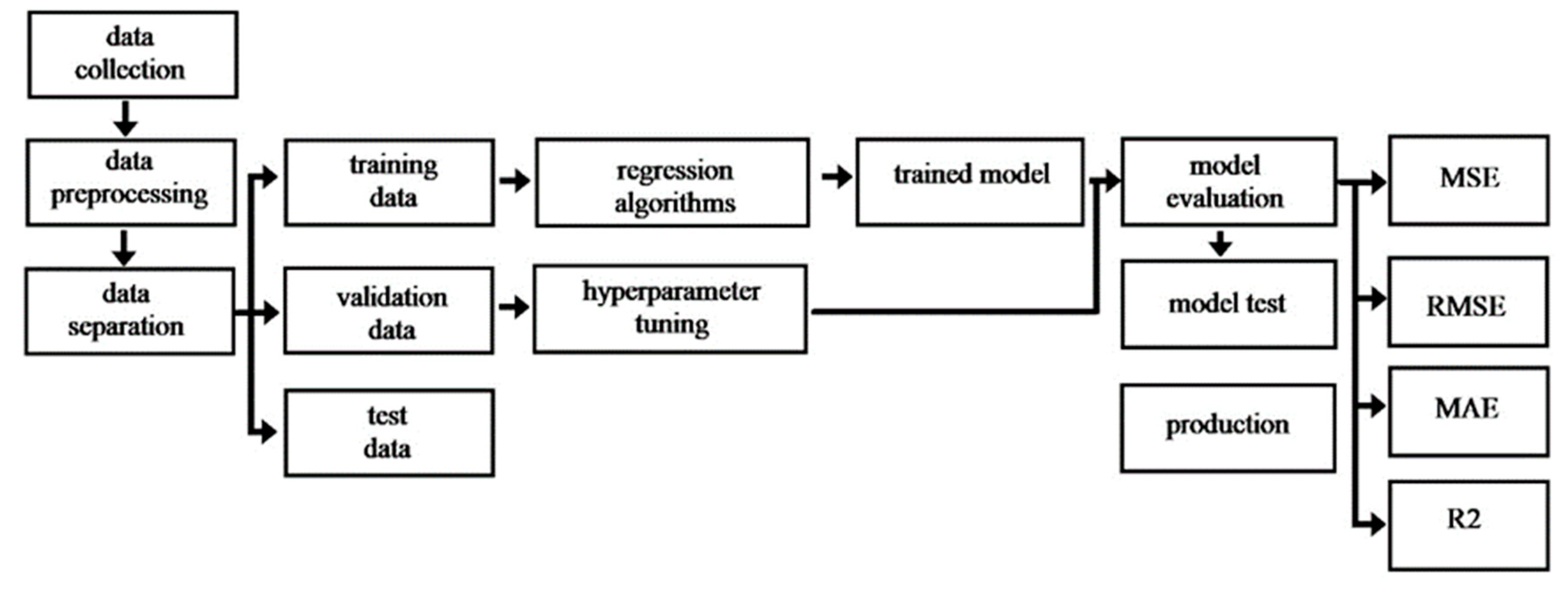
3.1. Machine Learning Approach Basics

A commonly accepted definition of machine learning is “the process of making computer systems to learn and improve by themselves without being specifically programmed”. Machine learning designs algorithms that automatically gather data and use them to learn. The supervised machine learning builds models that make predictions based off the knowledge provided. Adaptive algorithms identify patterns in the given data and “learn” from them. Then, they use this knowledge to generate reasonable predictions for new data. As an algorithm is provided with more known data, the predictive performance is improved [27]. Input data quality in terms of consistency and accuracy is crucial in machine learning. The uncertainty of input data heavily affects the validity of the results. The basic steps that are needed for completion of any supervised learning task are the following [28,29]:
  • Collection of the labeled data that will be used for training;
  • Determination of input and output features;
  • Preprocess of the labeled input data;
  • Separation of these data into three groups: training, validation and test data sets;
  • Determination of the suitable algorithm for the model;
  • Optimization of the parameters that affect the operation of the above algorithm (hyperparameter optimization);
  • Validation of the model;
  • Test of the prediction accuracy of the model by providing the test set;
  • Model ready for new predictions.
In Figure 1, we present the basic flow diagram of a supervised machine learning approach.

3.2. Basic ML Algorithm Categories Used for Regression

By far, the most commonly used algorithm for supervised regression problems in machine learning is the artificial neural network (ANN). They consist of a number of simple and internally interconnected processing units, which are organized in layers [30]. The first layer is always the input layer. We can then have different intermediate (hidden) layers, and then, the last layer is the output layer. In Figure 2, we present a common structure of an ANN.
At the core of every ANN is the neuron, which is the processing element. Each neuron receives signals, (from other neurons in previous layers or input signals from the external world) processes them, and outputs a signal to the next neuron or to the external world if it belongs to the output layer. In Figure 3, we present the inner structure of a neuron.
The neuron receives inputs (x0 to xq) that are multiplied with weights (w0 to wq). The weights represent the “strength” of the interconnection between the neurons, in other words the importance of each input. The weighted inputs are summed by the transfer function f(x).
f ( x ) = i = 1 q ( x i w i )
The above sum is used as input into the activation function, which is also a transfer function that is used to obtain the desired output for the problem designed. The importance of the activation function lies in the need for “breaking” the linearity in order for the neuron to output if this summation exceeds a predefined threshold value. The most commonly used activation functions are represented in Figure 4.
Another algorithm used for regression is polynomial Regression. It is a form of regression analysis in which the relationship between the independent variables and dependent variables is modeled by an n-th degree polynomial [31,32]. This algorithm is trying to fit a line that better “describes” the requested (predicted) values by tuning the coefficients of a n-th degree polynomial equation.
y = a 0 + a 1 x 1 + a 2 x 2 2 + + a n x n n
where y is the independent value (may be the ships actual speed), x1 to xn are the input data (the different factors that affect speed such as engine power, sea conditions, etc.), and a0 to an are the coefficients (the factor by which each of the input data affect the independent value).
Next in line is support vector regression (SVR), in which the algorithm aims at the reduction of prediction error by determining a hyperplane that minimizes the range between the predicted and the true values [33]. The objective of the SVR is to find a hyperplane in an nth-dimensional space (where n is the number of different input values) that fits in the maximum number of data points. This hyperplane is a complex form that is used to predict the values of the task that it is used (actual ship speed). Although SVC might seem to resemble polynomial regression, the basic idea is quite different. Polynomial regression tries to minimize the error rate, while SVC is fitting the error inside a certain threshold, which means that SVC approximates the best values within a given margin, called ε, as shown in Figure 5.
Given the training data in the form of Equation (3), the algorithm is trying to minimize Equation (4) under the constraints of Equation (5), where b and c are parameters.
( x i   y i )   i = 1 . y = w x + b
1 2 w 2 + c i = 1 m ( ξ 1 ι ξ 2 ι )
{ y i ( w x i ) b ε + ξ 1 i ( w x i ) + b y i ε + ξ 2 i ξ 1 i , ξ 2 i   0  
A different category of machine learning algorithms that is commonly used is the tree-based algorithm. Decision tree (DT) is the basic form of this kind of algorithm. The structure of these algorithms resembles a tree (thus, the name). The goal is to create a model that predicts the value of a target variable implementing simple decision rules inferred from the data features [34]. A more sophisticated tree-based algorithm is random forest (RF). Random forest combines a number of decision trees on various subsets of the given data set and calculates the average of each result to improve the predictive accuracy of that data set. By implementing the above rules, the algorithm can predict an independent value (once again: actual ship speed) by combining the different results that have been learned given the different input data (dependent values—factors that affect that speed).

3.3. Prediction Assessment Metrics

To establish a comparison framework among the different approaches, a common metric must be identified. The accuracy of a prediction is mathematically defined as the total number of correct predictions divided by the total number of predictions made for a specific data set. This definition is not valid in a regression problem (the ML problems where the output variable is a real or integer number) because we are seeking to predict the specific value of an attribute. In order to set limits on the deviation of predicted values and compare the results, several metrics have been introduced. The most commonly used in the literature are:
  • Mean absolute error (MAE). It is the average of the absolute differences between predictions and actual (true) values of the attribute of interest [35]. If N is the number of observations, y i is the actual (true) value, and y i is the predicted one. Then, the mathematical equation of MAE is:
    M A E = 1 N i = 1 N | y i y i |
  • Mean squared error (MSE). MSE takes the average of the square of the difference between predictions and actual (true) values. Because of the use of error squares, the effect of larger errors becomes more pronounced. The mathematical equation of MSE is:
    M S E = 1 N i = 1 N ( y i y i ) 2
  • Root mean squared error (RMSE). This is the square root of MSE. RMSE is more sensitive to variance than MAE because it is more affected by outliers in the results [30]. RMSE is mathematically expressed with the following equation:
    R M S E = 1 N i = 1 N ( y i y i ) 2
  • Finally, R square (R2). This focuses more on the operation of the algorithm and not on the results. It specifies the degree to which any variations in the values of the dependent variable (target attribute) can be explained by changes in the values of the independent variables (data set). If y i is the mean of all values, then it is mathematically expressed as:
    R 2 = 1 i ( y i y i ) 2 i ( y i y i ¯ ) 2

4. Implementation of Machine Learning in Ship Performance Prediction

4.1. Input Data Sources

As already mentioned, the first step in the machine learning procedure is data collection. For this purpose, when ship performance is of interest, the main sources for collecting the data needed are the following:
  • Noon reports;
  • Data acquisition systems (DAS) installed on board;
  • Meteorological ocean data from weather services;
  • Route data from Global Positioning System (GPS) or Automatic Identification System (AIS);
  • Hybrid methods;
  • Databases/simulated by external software.
Noon reports are manual readings/entries by the crew that are conducted once every day. Noon reports must include weather data that constitute an estimate of the crew. This method is the dominant in shipping companies worldwide [36]. The next method of data acquisition is systems installed on ships that collect and store data from various sensors on board. These systems have the advantage of a much higher sampling frequency, usually in the range of 15 s. This sampling rate is in accordance with ISO 19030. The next advantage of the data acquisition systems is accuracy. The minimum accuracy of the necessary sensors on board ships to fulfil the demands of ISO 19030 must be in the range of 0.1% to 5% [37]. Metocean data from weather services is another data source. It contradicts with the crew weather subjective estimations that usually lack accuracy. The term “hybrid” method refers to all analytical/semi empirical/CFD methods and trials that can be used as data sources. The last source of data for data-driven models is widely known databases arising from common-type vessels and data that arise from simulation software (mainly for research projects). Researchers use these databases as reference. In Table 2, we present the different data types and sources used in the studies that this paper compares.

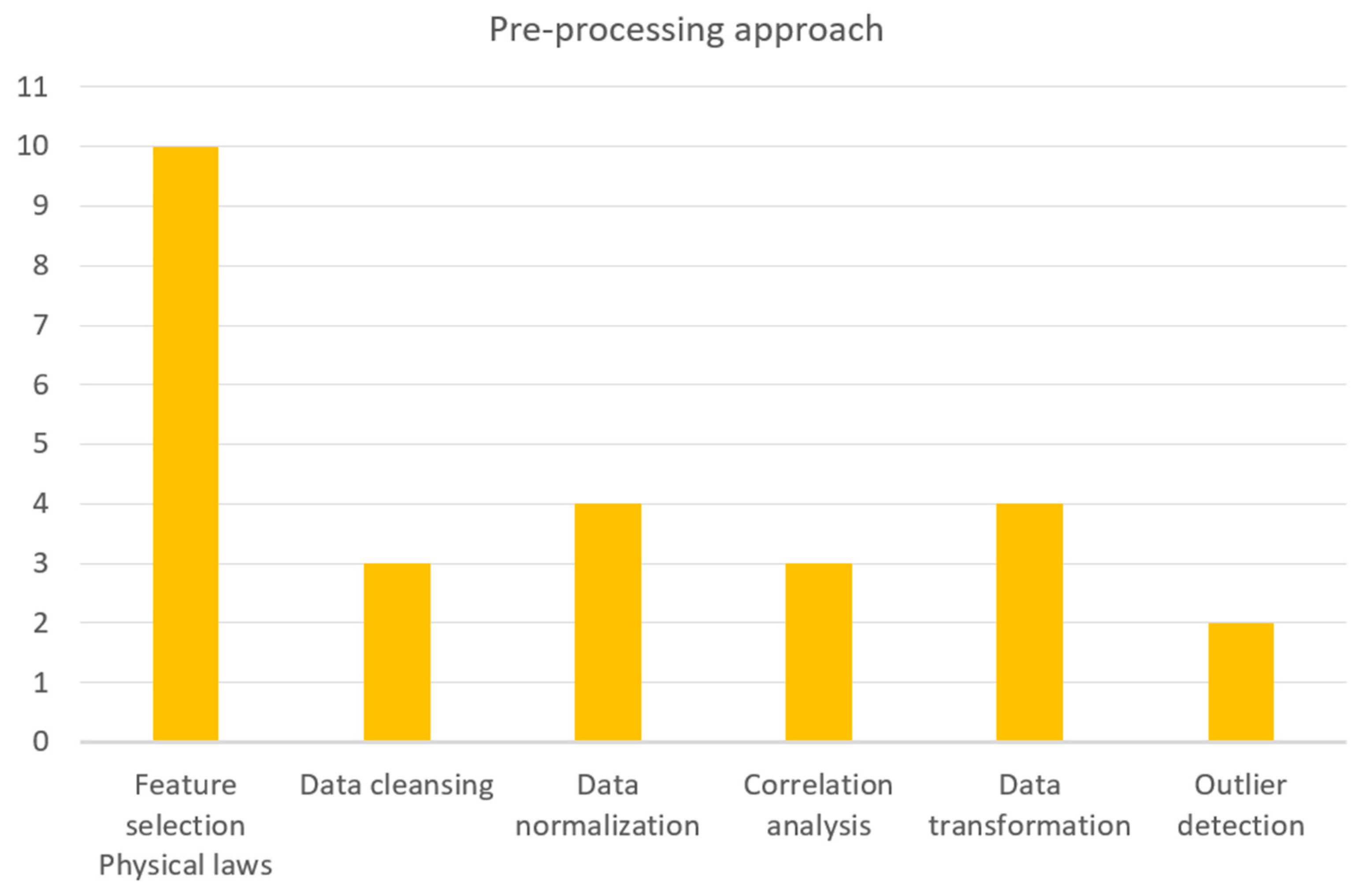
4.2. Preprocessing Methods

Data preprocessing is the next crucial step in the data-driven models. The data set that has been formed from the collected data can be used “as is” to train the machine learning algorithms or can be preprocessed [51]. The aim of the preprocessing is to reduce the size of the data set (and thus make it easier to handle) and to increase the prediction accuracy of the algorithms by removing misleading “noisy” input data. Big data sets with many input features (increased dimensions of the feature space) may lead to sparsity, and although it may seem to be a contradiction, it can negatively affect the prediction capability of machine learning algorithms. The so-called “curse of dimensionality” describes this phenomenon [52]. The most common preprocessing procedures are:
  • Feature selection driven by physical laws;
  • Feature selection with the use of a high correlation filter;
  • Correlation analysis;
  • Data normalization;
  • Data cleansing using clustering;
  • Data cleansing by operational limitations;
  • Feature engineering; data transformation based on physical laws;
  • Downsampling input data by calculating the average values;
  • Principal component analysis (PCA) to reduce the dimensionality;
  • Outlier detection and discarding based on z-scores.
In Table 3, we show the data preprocessing approach in the studies examined.

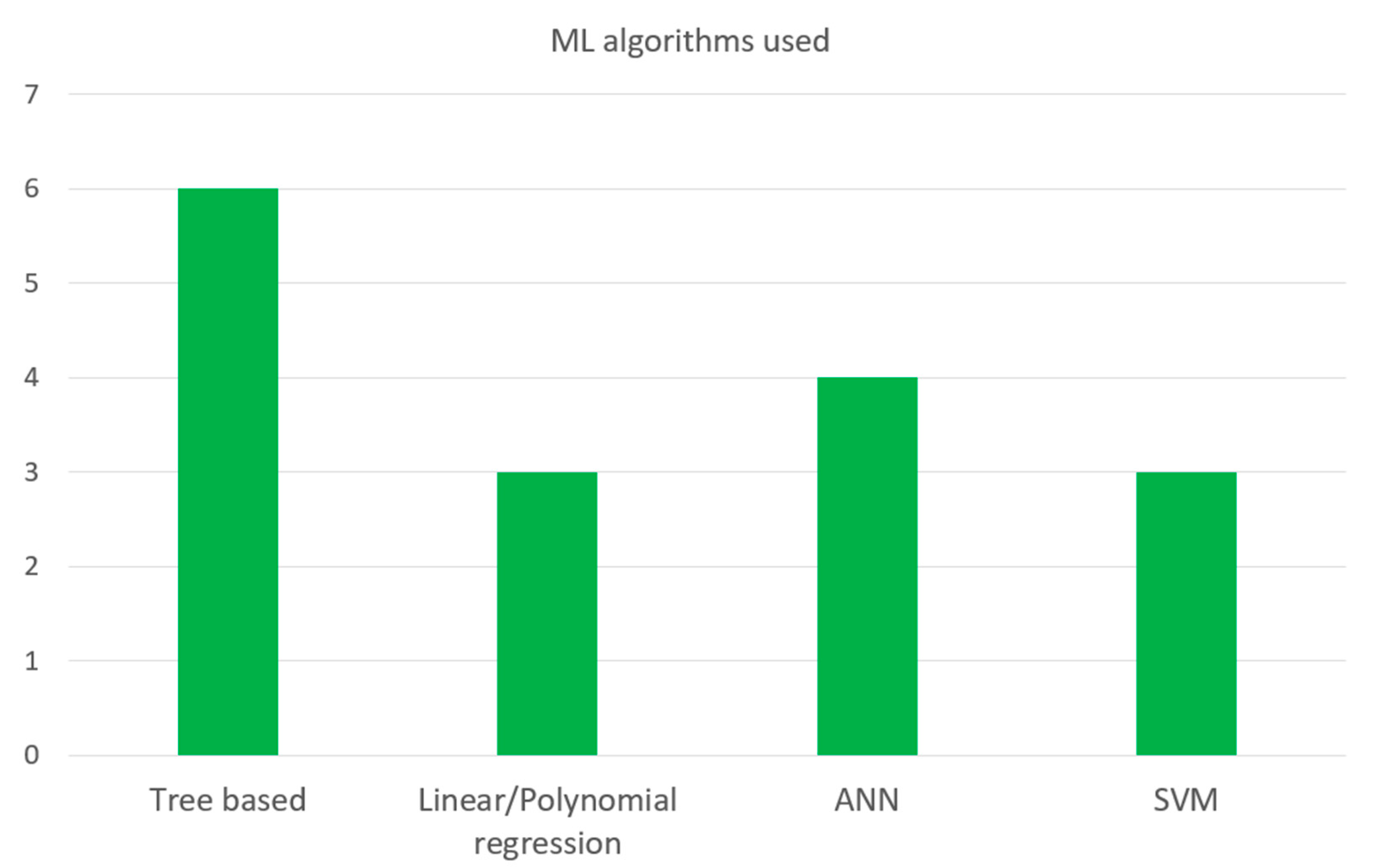
4.3. ML Algorithms Used/Hyperparameter Tuning

The selection of the proper machine learning algorithms is the next decision to be made. Most of the algorithms that are used in ship performance prediction belong to one of the three main categories that are presented in Section 3.2. Artificial neural networks are the dominant choice of the studies that are reviewed in this paper, and the authors believe that this observation reflects the overall modern trend. Generalized Regression Neural Network (GRNN), Multilayer Perceptron (MLP), Radial Basis Function Network (RBF), Linear Network, and Deep Extreme Learning Machine ANN represent the different ANN networks that are used. Regression Trees, Random Forests, Extreme Gradient Boosting Trees, Extra Trees Regressor are the tree-based algorithms used and Linear Regression, Support Vector Regression, Polynomial Regression, Generalized Additive Model, XGBoost, Gaussian Process Regression, Multiple Linear Regression, Projection Pursuit Regression are the regressors. Discrete Fracture Network, Adaptive Neuro-Fuzzy Inference and Generalized Additive Models are the three algorithms that complete the list and cannot be classified in any of the above categories [29,30,53].
Hyperparameters are the parameters of a machine learning algorithm that affect the prediction accuracy. The “No Free Lunch Theorem” [54] states that there is not one global architecture or parameter combination that performs best on a variety of machine learning tasks. It is of absolute importance to conduct hyperparameter tuning in order to optimize each specific task. The most commonly used method of optimization is grid searching. All the potential combinations of the chosen hyperparameters are tested, and the best combination is chosen. This method might lead to a substantial computational work because of the extremely high absolute number of combinations that may have to be evaluated. To address the above problem and in order to limit the computational workload, we can use the random search method. This method does exactly what it sounds, random combinations of hyperparameter settings are chosen, and the best configuration using trial and error qualifies. Another more elegant optimization approach is a model-based method using Bayesian optimization. The Bayesian theorem is used to adaptively generate data for hyperparameters and find the optimum hyperparameter values using surrogate models.
In Table 4, we present the different algorithms and the hyperparameter strategies (if stated) used in the studies reviewed in this paper.

4.4. Validation/Verification

In order to validate the performance of ML algorithms, there are two main approaches. First, there is the option to extract a relatively small portion of data from the complete data set and use it as the validation data set as presented in Figure 1. This option is commonly used but has the disadvantage of restricting the data set used for algorithm training. The second approach is cross validation. The k-fold validation method, which is representative of this category, separates the complete data set into k number of folds. One-fold is used as the test set and the sum of the other k-1 folds as a training set. The fold that is used as a test set alternates, and thus, we are able to validate the overall performance without the need to extract any portion of the data set from the training procedure.
For verification of the results, the prediction assessment metrics that are discussed in Section 3.3 or the results can be compared with the outcome of one of the other predictive methods that are presented in Section 2.
The validation of the different methods along with the results are presented in Table 5.

5. Discussion

From the comparison of the data-driven models that are used in the presented studies, we can discern a trend toward data acquisition systems as the means for the collection of input parameters. In 6 out of 15 papers, these systems are used to provide the input data. Conversely, noon reports, although they constitute the dominant method of collecting operational data in shipping companies, have been used in only 2 of the 15 papers. The beneficial effect of the higher frequency that is provided by the data acquisition systems on ships is perceived. Another interesting conclusion can be extracted from Table 1. The use of metocean data from various online services seems to be preferred against the onboard sensors or the crew estimations. In more than half of the papers, the environmental data needed were collected from online metocean services, even in the cases where the necessary sensors for the collection of environmental data were installed on board, as shown in Figure 6.
Regarding the preprocessing approaches that have been used, we can see that the dominate trend is toward feature selection driven by physical laws. Purely computational methods such as principal component analysis, that do not take into account the underlying physical phenomena, were not trusted by the majority of the researchers. In 66.7% of the cases, the physical laws governing the movement of the ship in the water were used in the formation of the data set that had been used, as shown in Figure 7.
Another interesting conclusion is that ANN, in various forms, seems to be the machine learning algorithm of choice (73.3% of the reviewed studies that deal with the prediction of ship performance used at least one form of ANN). ANN algorithms have gained popularity in recent years because the increased computational power needed for their implementation is now available with relative low cost. The main disadvantage of the methods that rely on ANN is that these algorithms need a vast amount of data in order to be trained. Except for the traditional fields that make use of these methods such as disease diagnosis, speech recognition and image classification (where the vast amount of input data is not an issue), the shipping industry with the adoption of data acquisition systems has begun to benefit from these methods. The other three categories of ML algorithms demand far less computational power and are more robust to the lack of huge data sets, as inputs can be a good alternative where the computational power or the data acquisition method used does not produce the necessary amount of data. These methods can and are being used (with slight method modifications) in computer science for email spam and malware filtering, as online fraud detection systems, among others, and in finance for stock market trading, to name a few. This if the main advantage of the different data-driven methods; unrelated scientific and industrial fields can benefit from the experience being built. In Figure 8, we present the frequency of implementation of the different ML algorithms used.
The hyperparameter tuning comparison is indistinguishable regarding the preferred method. Grid search, random search and Bayesian optimization alternate in the reviewed studies, without being able to identify any specific preference.
The benchmark metrics indicate a better accuracy when some form of ANN machine learning algorithm is used. In the papers where ANNs are directly compared with other implementations in the same data set, ANNs always prevail. The most important observation is that the verification of these results mainly occurs with the use of prediction metrics. Only in three cases have the comparative results been presented between the various existing predictive approaches, i.e., data-driven models and/or semi-empirical models and CFD models. The authors believe that a direct comparison of the results between data-driven models and the other main categories of ship performance estimation models needs to be further explored.

6. Conclusions

The prediction/estimation of a ship’s total resistance in real weather conditions can lead to the prediction of the actual speed through water that this ship can achieve with a given amount of power, which is one of the most important performance indicators. The resistance in calm weather and the resistance due to wind are relatively easy to be estimated with good precision and with various numerical/semi-empirical methods, or in recent years, with computational fluid dynamics models. When the geometric parameters of the ship and the boundary conditions are known, CFD can achieve remarkable results in estimating ship resistance. Conversely, numerical/semi-empirical methods are well developed and can estimate ship resistance with a good approximation and speed. Things become far more complicated when having to approximate the resistance of a ship in real weather conditions. The knowledge of the sophisticated geometric parameters of a ship or educational background in naval architecture is not necessary. When enough representative historical data of ship performance are available, these methods can estimate the ship speed performance with comparable or in some cases even better results. Due to their nature, semi-empirical and CFD are the methods of choice for shipyards, and data-driven models better suit the needs of shipping companies. From the study of the above ML approaches, we can conclude with relative certainty:
  • Increased frequency methods (onboard data acquisition systems) are starting to replace noon reports as the data input method of choice.
  • The new data acquisition systems that are installed onboard ships paved the way for the implementation of methods that rely on complex ML algorithms that achieve remarkable results. These algorithms were the privilege of other scientific fields until recently.
  • Researchers prefer to use methods for data preprocessing that rely on physical laws rather than purely computational alternative methods.
  • The above preference for research studies with physical laws as a tool for various steps in the data-driven methods pipeline indicate that the computational tools are not a good alternative for this application and must be improved upon in the future.
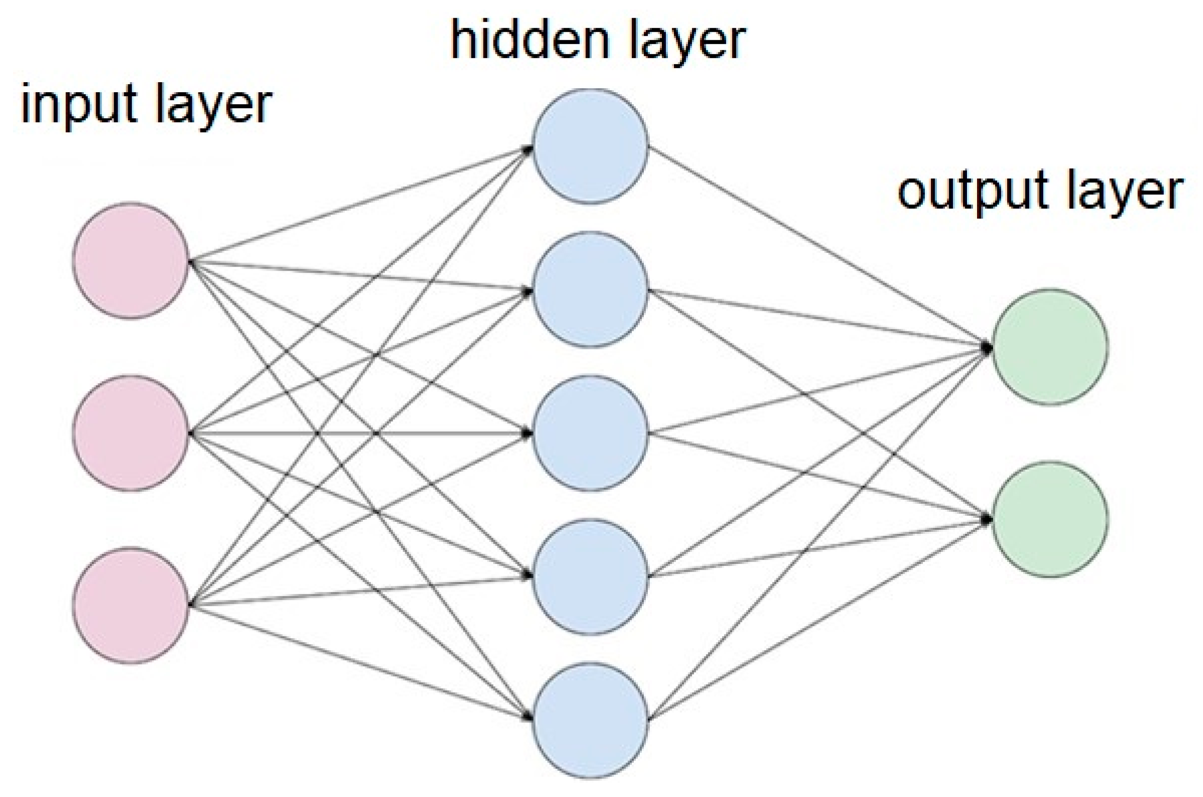
  • ANNs in various forms are starting to dominate as the ML algorithm of choice mainly due to the increased computational power available.
  • The accuracy of the prediction results of data-driven models is starting to increase in levels that offer a credible alternative for practical implementations.
  • In the absence of specific information of ship design (which is usually the prerogative of the shipyards that built the ship), which are necessary for implementing CFD or other deterministic methods, ML algorithms can currently fill the gap in predicting ship performance.
  • The “universal” nature of data-driven methods and the fact that computer science drives the evolution of these methods at a fast pace can lead to the total domination of these methods in shipping.
  • The level of uncertainty of input data heavily increases when implementing data-driven methods in real weather conditions. This drawback creates a demand for the development of specific preprocessing procedures in the future.

Author Contributions

Conceptualization, K.A., E.G.P. and H.C.L.; Data curation, K.A.; Formal analysis, K.A. and E.G.P.; Investigation, K.A., E.G.P. and H.C.L.; Methodology, K.A. and E.G.P.; Project administration, H.C.L. and E.G.P.; Software, K.A.; Validation, T.C.Z.; Writing—original draft, K.A.; Writing—review and editing, K.A., E.G.P., T.C.Z. and H.C.L. All authors have read and agreed to the published version of the manuscript.

Funding

Part of this research has been conducted under a project co-financed by the European Union and Greek national funds through the Operational Program Competitiveness, Entrepreneurship and Innovation, under the call RESEARCH–CREATE–INNOVATE (project code: T2EDK-03241).

Institutional Review Board Statement

Not applicable.

Informed Consent Statement

Not applicable.

Data Availability Statement

Not applicable.

Conflicts of Interest

The authors declare no conflict of interest.

References

  1. Oil 2021 Analysis and Forecast to 2026, International Energy Agency; IEA Publications: Paris, France, 2021.
  2. IMO. Initial IMO Strategy on Reduction of GHG Emissions from Ships; Resolution MEPC: London, UK, 2018; p. 304. [Google Scholar]
  3. IMO. Guidelines on the Method of Calculation of the Attained Energy Efficiency Design Index (EEDI) for New Ships; MEPC: London, UK, 2014; Volume 245. [Google Scholar]
  4. IMO. Guidance for Voluntary Use of the Ship Energy Efficiency Operational Indicator (EEOI); MEPC: London, UK, 2009. [Google Scholar]
  5. IMO. Guidelines for the Development of a Ship Energy Efficiency Management Plan (SEEMP); MEPC: London, UK, 2016. [Google Scholar]
  6. IMO. Guidance on Treatment of Innovative Energy Efficiency Technologies for Calculation and Verification of the Attained EEDI and EEXI; MEPC: London, UK, 2021. [Google Scholar]
  7. IMO. Guidelines on the Operational Carbon Intensity Rating of Ships (CII Rating Guidelines, G4); MEPC: London, UK, 2021. [Google Scholar]
  8. Carlton, J. Marine Propellers and Propulsion, 4th ed.; Butterworth-Heinemann: Oxford, UK, 2012. [Google Scholar]
  9. Kuroda, M.; Takagi, K.; Tsujimoto, M.; Fujisawa, J. Measurement of Added Resistance in Irregular Waves and Estimation of the Long-period Components. Jpn. Soc. Nav. Archit. Ocean. Eng. 2017, 24, 181–188. [Google Scholar]
  10. Kundu, P.K.; Cohen, I.M.; Dowling, D.R. Fluid Mechanics, 6th ed.; Elsevier Academic Press: Cambridge, MA, USA, 2016. [Google Scholar]
  11. Patey, M. Performance Monitoring Information Feedback to Design. In Proceedings of the 4th Hull Performance & Insight Conference, Gubbio, Italy, 6–8 May 2019. [Google Scholar]
  12. Logan, K.P. Using a ship’s propeller for hull condition monitoring, ASNE Intelligent Ships Symp, IX. Philadelphia 2011, 124, 71–87. [Google Scholar]
  13. Gkerekos, C.; Lazakis, I.; Theotokatos, G. Machine learning models for predicting ship main engine Fuel Oil Consumption: A comparative study. Ocean. Eng. 2019, 188, 106282. [Google Scholar] [CrossRef]
  14. Wang, J.; Bielicki, S.; Kluwe, F.; Orihara, H.; Xin, G.; Kume, K.; Feng, P. Validation study on a new semi-empirical method for the prediction of added resistance in waves of arbitrary heading in analyzing ship speed trial results. Ocean. Eng. 2021, 240, 109959. [Google Scholar] [CrossRef]
  15. Sasa, K.; Chen, C.; Fujimatsu, T.; Shoji, R.; Maki, A. Speed loss analysis and rough wave avoidance algorithms for optimal ship routing simulation of 28,000-DWT bulk carrier. Ocean. Eng. 2021, 228, 108800. [Google Scholar] [CrossRef]
  16. Liu, L.; Chen, M.; Wang, X.; Zhang, Z.; Yu, J.; Feng, D. CFD prediction of full-scale ship parametric roll in head wave. Ocean. Eng. 2021, 233, 109180. [Google Scholar] [CrossRef]
  17. Lang, X.; Mao, W. A semi-empirical model for ship speed loss prediction at head sea and its validation by full-scale measurements. Ocean. Eng. 2020, 209, 107494. [Google Scholar] [CrossRef]
  18. Kim, M.; Hizir, O.; Turan, O.; Day, S.; Incecik, A. Estimation of added resistance and ship speed loss in a seaway. Ocean. Eng. 2017, 141, 465–476. [Google Scholar] [CrossRef] [Green Version]
  19. Sulovsky, I.; Prpic-Oršic, J. Mathematical Model of Ship Speed Drop on Irregular Waves; University of Rijeka: Rijeka, Croatia, 2021. [Google Scholar]
  20. Liu, S.; Papanikolaou, A. Prediction of the Side Drift Force of Full Ships Advancing in Waves at Low Speeds. Mar. Sci. Eng. 2020, 8, 377. [Google Scholar] [CrossRef]
  21. Korkmaz, K.B.; Werner, S.; Bensow, R. Verification and Validation of CFD Based Form Factors as a Combined CFD/EFD Method. Mar. Sci. Eng. 2021, 9, 75. [Google Scholar] [CrossRef]
  22. Gao, Q.; Song, L.; Yao, J. RANS Prediction of Wave-Induced Ship Motions, and Steady Wave Forces and Moments in Regular Waves. Mar. Sci. Eng. 2021, 9, 1459. [Google Scholar] [CrossRef]
  23. Ntouras, D.; Papadakis, G.; Belibassakis, K. Ship Bow Wings with Application to Trim and Resistance Control in Calm Water and in Waves. Mar. Sci. Eng. 2022, 10, 492. [Google Scholar] [CrossRef]
  24. Inno, G.; Michael, S.; Hrvoje, J. Investigating Trim Optimisation in Waves for an AFRAMAX Tanker Using CFD. In Proceedings of the 5th Hull Performance & Insight Conference, Tullamore, Ireland, 26–28 October 2020. [Google Scholar]
  25. Inno, G.; David, B. Calculating Speed Loss Due to Swell using CFD. In Proceedings of the 6th Hull Performance & Insight Conference, Pontignano, Italy, 30 August–1 September 2021. [Google Scholar]
  26. Shigunov, V.; el Moctar, O.; Papanikolaou, A.; Potthoff, R.; Liu, S. International benchmark study on numerical simulation methods for prediction of maneuverability of ships in waves. Ocean Eng. 2018, 165, 365–385. [Google Scholar] [CrossRef]
  27. Alexiou, K.; Pariotis, E.G.; Zannis, T.C.; Leligou, H.C. Prediction of a Ship’s Operational Parameters Using Artificial Intelligence Techniques. Mar. Sci. Eng. 2021, 9, 681. [Google Scholar] [CrossRef]
  28. Aurelien, G. Hands-on Machine Learning with Scikit-Learn, Keras, and TensorFlow; O’Reilly Media, Inc.: Sebastopol, CA, USA, 2019; ISBN 978-1-492-03264-9. [Google Scholar]
  29. Andriy, B. The Hundred-Page Machine Learning Book; Andriy Burkov: Quebec City, QC, Canada, 2019; ISBN 978-1-9995795-0-0. [Google Scholar]
  30. Haykin, S. Neural Networks: A Comprehensive Foundation; Prentice Hall: Hoboken, NJ, USA, 1999. [Google Scholar]
  31. Abhigyan. Retrieved from Understanding Polynomial Regression. Available online: https://medium.com (accessed on 2 August 2020).
  32. Fan, J. Local Polynomial Modelling and Its Applications: From linear regression to nonlinear regression. In Monographs on Statistics and Applied Probability; Chapman & Hall/CRC: Boca Raton, FL, USA, 1996. [Google Scholar]
  33. Cortes, C.; Vapnik, V. Support-Vector Networks. Kluwer Acad. Publ. 1995, 20, 273–297. [Google Scholar] [CrossRef]
  34. What is a Decision Tree? Available online: https://towardsdatascience.com/what-is-a-decision-tree-22975f00f3e1 (accessed on 1 June 2022).
  35. Abebe, M.; Shin, Y.; Noh, Y.; Lee, S.; Lee, I. Machine Learning Approaches for Ship Speed Prediction towards Energy Efficient Shipping. Appl. Sci. 2020, 10, 2325. [Google Scholar] [CrossRef] [Green Version]
  36. Gonzalez, C.; Lund, B.; Hagestuen, E. Case Study: Ship Performance Evaluation by Application of Big Data. In Proceedings of the 3rd Hull Performance & Insight Conference, Durham, UK, 12–14 March 2018. [Google Scholar]
  37. ISO 19030; Ships and marine technology—Measurement of changes in hull and propeller performance. ISO: London, UK, 2016.
  38. Cepowski, T. The prediction of ship added resistance at the preliminary design stage by the use of an artificial neural network. Ocean Eng. 2019, 195, 106657. [Google Scholar] [CrossRef]
  39. Duan, W.; Yang, K.; Huang, L.; Jing, Y.; Ma, S. A DFN-based method for fast prediction of ships’ added resistance in heading waves. Ocean. Eng. 2020, 245, 110484. [Google Scholar] [CrossRef]
  40. Tarelko, W.; Rudzki, K. Applying artificial neural networks for modelling ship speed and fuel consumption. Neural Comput. Appl. 2020, 32, 17379–17395. [Google Scholar] [CrossRef]
  41. Lang, X.; Wu, D.; Mao, W. Comparison of supervised machine learning methods to predict ship propulsion power at sea. Ocean. Eng. 2022, 245, 110387. [Google Scholar] [CrossRef]
  42. Antonic, R.; Valcic, M.; Tomas, V. Ship speed prediction in real sea environment using advanced technologies. In Proceedings of the 11th WSEAS International Conference on Applied Computer and Applied Computational Science Conference, Rovaniemi, Finland, 18–20 April 2012. [Google Scholar]
  43. Bassam, A.M.; Phillips, A.B.; Turnock, S.R.; Wilson, P.A. Ship speed prediction based on machine learning for efficient shipping operation. Elsevier 2022, 245, 110449. [Google Scholar] [CrossRef]
  44. Brandsæter, A.; Vanem, E. Ship speed prediction based on full scale sensor measurements of shaft thrust and environmental conditions. Elsevier 2018, 162, 316–330. [Google Scholar] [CrossRef] [Green Version]
  45. Tran, T.A. Comparative analysis on the fuel consumption prediction model for bulk carriers from ship launching to current states based on sea trial data and machine learning technique. J. Ocean Eng. Sci. 2021, 6, 317–339. [Google Scholar] [CrossRef]
  46. Mittendorf, M.; Nielsen, U.D.; Bingham, H.B. Data-driven prediction of added-wave resistance on ships in oblique waves—A comparison between tree-based ensemble methods and artificial neural networks. Appl. Ocean. Res. 2022, 118, 102964. [Google Scholar] [CrossRef]
  47. Coraddu, A.; Oneto, L.; Baldi, F.; Cipollini, F.; Atlar, M.; Savio, S. Data-driven ship digital twin for estimating the speed loss caused by the marine fouling. Ocean. Eng. 2019, 186, 106063. [Google Scholar] [CrossRef]
  48. Yan, R.; Wang, S.; Du, Y. Development of a two-stage ship fuel consumption prediction and reduction model for a dry bulk ship. Elsevier 2020, 138, 101930. [Google Scholar] [CrossRef]
  49. Moreira, L.; Vettor, R.; Guedes Soares, C. Neural Network Approach for Predicting Ship Speed and Fuel Consumption. Mar. Sci. Eng. 2021, 9, 119. [Google Scholar] [CrossRef]
  50. Lee, J.B.; Roh, M.I.; Kim, K.S. Prediction of ship power based on variation in deep feed-forward neural network. Int. J. Nav. Archit. Ocean. Eng. 2021, 13, 641–649. [Google Scholar] [CrossRef]
  51. Kiriakos, A.E.P. Comparative evaluation of Machine Learning algorithms and Physical based models for the prediction of Vessel Speed in real life applications. In Proceedings of the PCI 2021: 25th Pan-Hellenic Conference on Informatics, Volos, Greece, 26–28 November 2021. [Google Scholar]
  52. Bellman, R. Rand Corporation. In Dynamic Programming; Princeton University Press: Princeton, NJ, USA, 1957. [Google Scholar]
  53. Shai, S.-S.; Shai, B.-D. Understanding Machine Learning: From Theory to Algorithms; Cambridge University Press: New York, NY, USA, 2014; ISBN 978-1-107-05713-5. [Google Scholar]
  54. Goodfellow, I.; Bengio, Y.; Courville, A.; Goodfellow, I.; Bengio, Y.; Courville, A. Deep Learning (Adaptive Computation and Machine Learning Series); The MIT Press: Cambridge, MA, USA, 2016; ISBN 0-262-03561-8. [Google Scholar]
Figure 1. Flow diagram of supervised machine learning.
Energies 15 06094 g001
Figure 2. ANN structure with one hidden layer.
Energies 15 06094 g002
Figure 3. Neuron inner structure.
Energies 15 06094 g003
Figure 4. Common activation functions.
Energies 15 06094 g004
Figure 5. SVC hyperplane.
Energies 15 06094 g005
Figure 6. Input data source usage.
Energies 15 06094 g006
Figure 7. Preprocessing approach usage.
Energies 15 06094 g007
Figure 8. ML algorithm usage.
Energies 15 06094 g008
Table 1. Publications that implement Semi-empirical formulas, model tests or CFD models.
Study (Reference)AimMethod UsedApplication SystemResults/Conclusions
[14]Validation of the SHOPERANTUA-NTU-MARIC (wave-added resistance prediction method.Semi-empirical (SNNM) validated by Pearson’s correlation coefficient R and mean square error (MSE)Model test results of 29 different type vesselsPearson correlation Coefficient R equal to 0.86 and 0.94. The relative error distribution μ = 0.0% and σ = 2.0%. Furthermore, 75% of samples are within ±2% intervals, and 93% of the samples are within ±4%, while almost all sample points are within ±6%.
[15]Simulation of optimal ship route with speed loss analysis in conditions including rough sea voyage.Semi-empirical. Comparison of the results with measurement data28,000 DWT-class bulk carrierResults vary with different weather conditions. Further validations are needed to produce more reliable simulations.
[16]CFD prediction of a full-scale ship parametric roll in a regular head
wave.
Reynolds-averaged Navier–Stokes (URANS) CFD, detached eddy simulation (DES), and large eddy simulation (LES).Container shipThe occurrence of parametric roll can be simulated well, and the roll amplitude and period can be predicted accurately.
[17]Semi-empirical model to estimate a ship’s speed loss at head sea.A proposed theoretical weather factor prediction modelPCTC and a chemical tanker.Sufficiently accurate approximations compared to the other existing well-known approaches.
[18]Prediction of the added resistance and attainable ship speed under actual weather conditions2-D and 3-D potential flow method and CFD with unsteady Reynolds-averaged Navier–Stokes (URANS)Container shipNumerical results were found to agree reasonably well with the experimental data in regular head and oblique seas.
[19]Estimation of the speed of a vessel in rough seasSimplified analytical methodContainer shipAnalytical approximation has room for improvement.
[20]Analysis of the experimental results of the mean sway forces at low speeds in regular waves of various directionsEmpirical formulaSix full-type shipsEmpirical formula can satisfactorily capture the mean sway force acting on full-type ships, at both zero and non-zero low speeds.
[21]Prediction of the propulsive power of ships and comparison with 1978 ITTC Performance Prediction MethodCombination of towing tank EFD testing and CFD (Reynolds-averaged Navier–Stokes (RANS))Fourteen common cargo vesselsProposed method can provide immediate improvements to the 1978 ITTC Performance Prediction Method
[22]Prediction of the wave-induced motions, and steady wave forces and moments in regular head and oblique wavesCFD Reynolds-averaged Navier–Stokes (RANS)Oil tanker
KVLCC2
(1) The computed added resistance as well as the steady wave sway force and yaw moment with inertia effects due to the wave-induced motions agree well with the available experimental data.
(2) The comparison of the computed resistances using two wave amplitudes indicates that added resistance is not proportional to the square of wave amplitude.
(3) RANS solver can be used as a tool for ship seakeeping analysis.
[23]Test case focused on the resistance and thedynamic behavior of the wing–vessel configuration in calm water conditions and in head waves.Experiments conducted in the towing tank and
CFD.
Ferry ship hull model(1) Bow wing in static mode can be used for trim-control of a vessel by altering the angle of attack,
leading to a possible drop in wave resistance both in calm water and in waves.
(2) Utilizing the wing in head waves results in a significant reduction in the pitching and heaving responses of the vessel.
[24]Trim Optimization in WavesCFD simulation and use of JONSWAP spectrum to determine the individual wave componentsAFRAMAX TankerThere is an economic benefit in performing trim optimization studies for full hull forms, at least those sailing on longer routes.
[25]Investigation of speed lost due to swellCFD simulations using Stokes’ second wave theoryCapesize and Handysize vessel(1) With a minimum warranted speed of 13 kn, speed loss of the Capesize vessel is 0.67 kn, while for the Handysize vessel, it is 1.85 kn.
(2) More attention needs to be given to swell when observing the performance of a vessel.
Table 2. Data source and data type of related studies.
Study (Reference)Input Data SourceInput Data
[27]Data acquisition systemShip, engine data and environmental data from onboard sensors
[35]AIS and noon reportsShip operational data and metocean data
[38]Experimental researchGeometric parameters
[39]Experimental research and calculated dataGeometric parameters
[40]Experimental research and sea trialsShip operational data and metocean data
[41]Data acquisition systemShip operational data and metocean data
[42]Databasemetocean data
[43]Data acquisition systemShip operational data
[44]Data acquisition systemShip operational data and metocean data
[45]Data acquisition systemShip, engine data and metocean data
[46]Calculated dataGeometric parameters
[47]Data acquisition systemShip, engine data and environmental data from onboard sensors
[48]Noon ReportsShip, engine data and metocean data
[49]Simulated by route planning softwareEngine data and metocean data
[50]DatabaseShip operational data and ocean environmental data
Table 3. Data preprocessing approach in reviewed studies.
Study (Reference)Preprocessing Approach
[27]Feature selection driven by physical laws; data cleansing by operational limitations; data transformation based on physical laws; data normalization
[35]Feature selection driven by physical laws; outlier detection and discarded based on the z-scores; data cleansing by operational limitations; correlation analysis
[38]Feature selection driven by physical laws
[39]Data transformation based on physical laws, added extra input layer
[40]Data cleansing using clustering
[41]Feature selection driven by physical laws
[42]Feature selection driven by physical laws
[43]Correlation analysis; feature engineering: data transformation based on physical laws; data normalization
[44]Feature selection driven by physical laws; outlier detection and discarded based on the z-scores
[45]Feature selection driven by physical laws; correlation analysis
[46]Feature engineering; data transformation; data normalization
[47]Data normalization; downsampling input data by calculating the average values
[48]Feature selection driven by physical laws
[49]Data transformation based on physical laws
[50]Data transformation based on physical laws
Table 4. Algorithms and hyperparameter tuning methods used in the reviewed studies.
Study (Reference)Algorithm UsedTuning/Hyperparameter Tuning
[27]Random Forest, Linear Regression, K-NN, ANN, Decision Tree Regressor, AdaBoostYes/(Random)
[35]Decision Tree Regressor, Random Forest Regressor, Extra Trees Regressor, Gradient Boosting Regressor, Extreme Gradient Boosting RegressorYes (k-fold)
(Cross-validation)
[38]Generalized Regression ANN (GRNN), Multilayer Perceptron (MLP), Radial Basis Function Network (RBF), Linear NetworkNot Stated
[39]Discrete Fracture NetworkNot Stated
[40]Multilayer Perceptron (MLP) ANNNot Stated
[41]Linear Regression, Support Vector Regression, Polynomial Regression, Generalized Additive Model, XGBoost, ANNYes (Grid search)
[42]Adaptive Neuro-Fuzzy Inference ANFISNot Stated
[43]Multiple Linear Regression, Regression Trees, Support Vector Regression, Gaussian Process RegressionYes (Bayesian optimization)
[44]Linear Regression, Generalized Additive Models, Projection Pursuit RegressionNot Stated
[45]ANNNot Stated
[46]Random Forests, Extreme Gradient Boosting Trees, ANNYes (Bayesian optimization)
[47]Deep Extreme Learning Machine ANNYes (Algorithm adopting)
[48]Random ForestsNot Stated
[49]Multilayer Perceptron (MLP) ANNNot Stated
[50]Deep Feed-Forward ANNYes (trial and error)
Table 5. Validation and results of the different methods used.
Study (Reference)ValidationVerification
[27]Extracted validation data setMAE, MSE, RMSE, R2 (error less than 3%)
[35]Extracted validation data setMean absolute percentage error of the Random Forest regressor = 7.91%
[38]Extracted validation data setMSE values between 0.98 and 1.1 comparisons with STAWAVE-2
[39]Extracted validation data setRMSE (smaller approx. 10–12%)
[40]Extracted validation data setR2 > 0.95, 0.8–2.8% accuracy
[41]Extracted validation data setMAE, RMSE, R2 (XGBoost most stable and reliable predictive ability)
[42]Extracted validation data setRMSE = 0.161
[43]Cross validationMAE, MSE, RMSE, R2 comparison
[44]Cross validationLinear regression and generalized additive models increased accuracy of 16 and 12%
[45]Extracted validation data setR2 > 0.9055
Comparison with simulation software
[46]Cross validationRMSE, MAE comparison
Verified with numerical and experimental data
[47]Extracted validation data setBetter prediction accuracy and reliability, with respect to the ISO 19030
[48]Cross validationComparison with real values
[49]Extracted validation data setRMSE, R2 comparison
[50]Cross validationSatisfactory accuracy using as input data only the information about the sea conditions
Publisher’s Note: MDPI stays neutral with regard to jurisdictional claims in published maps and institutional affiliations.

